When the program execution passes through real instruction code, it joins ..... after some stay in segment j the program execution joins its normal instruction flow.
БЪЛГАРСКА
АКАДЕМИЯ
КИБЕРНЕТИКА И CYBERNETICS AND
НА
НАУКИТЕ.
BULGARIAN
ACADEMY
ИНФОРМАЦИОННИ ТЕХНОЛОГИИ, INFORMATION TECHNOLOGIES, 2
OF
SCIENCES
2
София . 2001 . Sofia
Processor Control-Flow Error-Detection Techniques Model and Evaluation Tool Edita Djambazova, Krassimir Djambazov Institute of Computer and Communication Systems, 1113 Sofia
Abstract: A model of computer system's behavior is presented with embedded tools for control flow error detection. The model is aimed at determining of the coverage factor of these tools and/or the techniques for their construction and of combinations of the techniques. The actual parametersof the evaluated system and the specific implementation characteristics of the error detection techniques/tools are considered in the model. The system behavior is presented as a probabilistic graph, where absorbing states are defined for which the specific coverage factors of the different techniques could be analytically determined. The timedependent model allows for simulation of the coverage factor as a function of time from the point of error occurence. On the basis of this model and evaluation tool is developed for coverage assessment at different design stages. To illustrate the abilities of the evaluation tool experimental results are presented obtained on a generalized system and the influence of some significant implementation characteristics of the different techniques is analized. Keywords: error detection techniques, coverage factor, simulation model.
1. Introduction The fault tolerance of computer systems can be achieved through error masking, error detection or combination of these approaches. Many fault-tolerant applications in computer systems are based on error recovery techniques rather than on error masking ones. The essential function in error recovery is the error detection. In fault-tolerant distributed control systems, fail-stop components (controllers) are often used. The fail-stop approach requires implementation of self-checking tools in controllers to stop the operation in case of error detection. The notion of coverage factor defines the ability of a computer configuration to detect errors in case of their occurrence. A good part of the error detection techniques are application specific that makes the coverage factor estimation strongly dependent on the actual system parameters. 3
Error detection techniques could be classified in two groups: functional and application oriented. The first group is aimed at checking the correct system operation. Two classes of functional methods could be distinguished: on-line checking and periodic functional tests. Application-oriented methods are used for error detection in control flow (program execution), mostly for application programs. The four main classes of application oriented methods are: time checking, control flow checking, results assessment, and exception handling. Time and control-flow checking are methods (and techniques) for concurrent error detection. Concurrent error detection techniques [9, 2] use program segmentation and points in each segment where some conditions are checked. The patterns for comparison are issued concurrently from an independent monitor on the basis of the history of computational process. Concurrent error detection techniques are: time checking of program execution[3, 10], checking of number of fetched instructions [6], checking of segments’ sequencing (assignedsignatures techniques) [5, 10, 7, 4], and checking of sum of instructions’ operational codes in the executed segment (derived-signatures techniques) [9, 11]. There are two directions in coverage assessment: modeling and measurement after fault injection. The second direction has the drawback to be a physical approach, i.e., a system prototype has to be available, the application software has to be programmed before the check whether the system meets its error detection requirements. The data for error detection techniques’ properties are strongly dependent on the setup of the experiment, on the error definitions and error models accepted, on the technical abilities of the setup, etc. The experimental results give only a basis for comparison of the implemented techniques and some insight for their operation in different environment. The design process implies the choice of a technique/method for error detection to be made at earlier design stages. To ease the preliminary assessment of the coverage factor, analytical and simulation models are applied. Unfortunately, most of the existing models are developed for assessment of a single method which makes the comparative analysis of the different techniques difficult. These models do not allow for estimation of the integral effect in case of combination of methods. Most of the known modeling approaches do not consider the influence of the application specifics on the coverage, thus ignoring the effect of the design solutions. Fault injection methods can give the time function of the coverage, while none of the known models could assess it. In Section 2 of the paper considerations about the importance of the time properties of the coverage are presented.
2. Goals of the study The definition of coverage factor concerns the probability an error occurrence to be detected within unlimited time interval. This definition is useful when the application does not pose time restrictions, i.e., if the definition of system failure is time-independent. We shall call the above definition static coverage factor. The dynamic coverage factor is presented as a time function of the probability for system failure detection. The coverage assessment model is purposed at considering some system properties, estimation of the integral effect of the implementation of different error detection techniques, and determining the dynamic coverage factor. In the concurrent error detection techniques, there is a dependence of the coverage upon factors specific to the application: processor’s instruction set, instruction coding, segment size, signature size, precision of the checking time intervals, program code size, data memory size, etc. Control flow errors are due to wrong interpretation of an instruction. There is a dependence between the instruction codes and the probability for erroneous instruction interpretation. The number of erroneous bits in an instruction should also be taken into account. System’s behavior after control flow violation depends on the size of the program code, the 4
data, and the free address space. Therefore, the memory distribution should also be included in the model. Parameters, specific to the application, such as signature size, segment size, precision of the checking time interval, are closely related to the coverage of the error detection techniques and should be included in the model. The implementation of combined techniques for error detection implies coverage assessment in case of intersection of detected error types. A clear distinction among the types of detected errors and definition of specific coverage factors for the different methods are needed. In the real-time systems, the control system’s failure is usually defined in terms of the error sojourn time referred to the time parameters of the object under control. In control systems, there is a time redundancy due to time delays of the object under control. The redundancy reflects the compensation property of the control system after some limited period of control loss. Therefore, the same error with the same duration could be a system failure in one application and no failure, in another. Following this consideration, in many cases the static definition of the coverage factor is insufficient for reliability estimation. The presented study includes: Definition of error model. Development of generalized model of erroneous behavior of computer system, according to the error model. Functional extension of the erroneous behavior model with the influence of error detection techniques. Definition of coverage function of error detection techniques. Analysis of time-dependent parameters in the erroneous behavior model of computer system. Transformation of the model for presentation of coverage function. Modeling program for determination of coverage function. Experiments with the models for coverage function and analysis of the results.
3. Generalized model of erroneous behavior of computer system 3.1. Introduction The model considers a system where error detection tools are implemented to check the correctness of control flow execution. It is assumed that after error occurrence the processor operation stops upon signal from the checking tools. The stop is either fail-stop or is followed by some recovery actions. The analytical determination of the coverage of the software/hardware error detection tools requires development of a system behavior model in case of error. The presented model differs from the known models in its orientation towards parameters that could be analytically derived from system’s characteristics. The effect of the applied checking tools is also considered. The model follows some assumptions: The program code is divided in program segments. The segments’ size and the criterion for its determination depend on the applied technique(s). Each fault causes an error in the data and may be error in operands, in code of operation or in instruction extension. The last error type could be in address (of operand or of instruction) or direct operand. The analysis considers errors that affect directly program’s control flow. Such transformations of the control flow are called unspecified transitions. The address space of the processor is divided in three parts: code, data, and free address space. Program code is placed in the code address space. Data address space does not contain any code. The rest address space is free.
5
3.2. Error model Errors are caused by faults that could be permanent or transient (self-recovering). Transient faults are classified as faults that cause dynamic and static errors. Dynamic errors pass after some time and cause a single change of information at the moment of its transmission or handling. Static errors are related to permanent change of the information stored in the system memory. The two classes of errors have equivalent effect and cause failures of the same type. Their differentiation is necessary to determine the probabilistic characteristics of unspecified transitions when we determine the total coverage factor. The probability of occurrence of unspecified transition is determined by two components: probability of dynamic error and probability of static error. For the dynamic component it is necessary to analyze the frequency of execution of each instruction and to determine the probability of its transformation during the execution of branch instruction, to analyze the frequency of execution of branch instructions and to determine the probability the address part of each branch instruction to be changed, as well as to determine the probability each instruction to be transformed into instruction with different length. The static component is related to change of data in the system memory that are code. In this case, the important factor is not the frequency of execution but the number of instructions and their distribution by types which could be changed causing an unspecified transition. Errors could be distinguished also by their observability by a monitor, operating concurrently with the processor. In this sense, all static errors are observable, while the part of the dynamic errors, caused by faults inside the processor, are unobservable. For some methods the inside/outside separation of dynamic errors is important when estimating the coverage of the techniques for different error types. The possible effects of erroneous interpretation of the original program code are presented in Table 1. The first column contains description of the affected part of instruction. Table 1 Affected part
Program Instruction
Changed Instruction
Detectable Error
Effect on Control Flow
Branch
Yes
Non-branch,
Yes*
-
Yes
Next segment transition
Unspecified transition
same length Non-branch
Non-branch, different length
Joining Unspecified transition
Instruction Code
Branch
Branch
Yes*
-
Non-branch, same length
Yes*
-
Yes
Next segment transition
Non-branch, different length
Joining Unspecified transition
Operand
Non-branch Branch
-
* Detectable if the error is observable by an external monitor.
6
Yes* Yes
Unspecified transition
code of operation or operand. The second column describes the instruction in the original program. Branch and non-branch instructions are considered since their wrong interpretation could change the control flow. In the third column the changes in the original instruction are presented. The column “Detectable Error” determines whether the error is detected by some of the applied methods. The effect of the erroneous interpretation on the control flow is shown in the last column of the table. When a program instruction is incorrectly interpreted as instruction with different length, the next fetched byte will not be an original instruction code and therefore an arbitrary data will be misinterpreted as code of operation. During such wrong program execution till the end of the current segment three events are possible. If the arbitrary data is interpreted as a branch instruction, an unspecified transition is performed. When the program execution passes through real instruction code, it joins the original control flow and the checkpoint of the segment is reached. If neither unspecified transition, nor joining of the original code happens, the wrong program execution linearly continues to the next segment. In this case, the checkpoint of the segment is skipped. In the model this transition is treated as unspecified transition into the physically next segment.
3.3. Generalized model of error detection The model is constructed in a way that allows for tracing the trajectory of the executed program to one of the absorbing states upon error. A probability corresponds to each path. The end states upon error could be of three classes: fully detectable, partially detectable, and undetectable. All classes are assigned to absorbing system states correspondingly. The state transition probabilities are defined on the basis of known system parameters and, thus, are calculable. The paths in the model represent error propagation from its occurrence to an absorbing state. The absorbing states are defined as states where errors are detected by the corresponding technique with known probability. States where the control flow passes a checkpoint are absorbing states with specific probability of error detection. These specific coverage factors depend on the detection technique(s) applied. Two models are developed: steady-state model and time-dependent model for coverage assessment.
3.3.1. States and transitions in the model In Fig. 1 the state diagram of the steady-state model is presented, comprising a set of states and transitions among them. The states and probabilities specific for the steady-state model are described in §3.3.3. The differences for the time-dependent model are shown in Fig. 2 and are discussed in §3.3.4. The diagram shows the system behavior when an error occurs during the execution of a program segment. The states represent: (i) cases of control flow’s erroneous redirection (unspecified transition, transition to the next segment or joining) and (ii) the specific further execution with regard to passing the checkpoints. The description of system’s behavior includes a set of states and transitions among them that are executed with respective probabilities pmn (from state Sm to state Sn). State S0 corresponds to error occurrence during execution of the i-th segment. The probability of occurrence of this event is pi. States S1, S2, and S3 are entered after execution of an unspecified transition (branch). The probability an error that has occurred during the execution of segment i to cause an unspecified transition is pi0. An unspecified transition could transfer the program execution in another program segment state S3 with probability pp, in the data space of the memory state S2 with probability pd, and in the free address spacestate S1 with probability pf . We assume that the transition in the free address space ends up with stopping of the processor in state S9. The transition in the data space of the memory ends up either with stopping of the processor in 7
state S9, or with transition towards a program segment (state S3 with probability pr). p01 = pi0pf ,
p02 = pi0pd,
p03 = pi0pp.
States S4 and S5 reflect the cases when after an error the program execution continues in program segment j either directly, or through intermediate transitions. The program execution can remain in the same segment – transitions from state S0 to states S4, S5, and S8. The probability for transition in segment j is pj. The transition into segment j could be on a code of operation state S4 with probability pj0 or on a byte with arbitrary contents state S5 with probability (1 pj0). p34 = pj pj0,
p35 = pj (1 pj0).
When the transition is on a byte which is not a code of operation, transitions to two absorbing states are possible: stop state S7 with probability p57 and absorbing checking state S6 after joining the code of segment j with probability p56=pcop. The other transitions are to the next program segment with probability pn and to the states of unspecified transition S1, S2, and S3 with probability p51 , p52 , p53 , correspondingly. Upon error that transforms an instruction into instruction with different length, the program execution remains in segment i. The probability for direct transition between state S0 and states S4 and S5, when i=j, is pdl. p04 = pdlpj0, p05 = pdl(1 - pj0)
for i = j.
When the error causes a transformation into instruction with the same length, a direct transition is made between state S0 and state S8 which corresponds to transition on the checkpoint of segment i with probability p08 = psl . When the program execution reaches the physically last segment a transition is possible into free address space that lies directly after the segment’s code. The probability for such transition is pn. Probability of error during execution of segment i pi = si psi + di pdi, si + di = 1, where si is a weight coefficient of static errors, di is a weight coefficient of dynamic errors. psi is the probability of static error in segment i. It is a function of li, the length of the code of segment i, and l, the total code length; pdi is the probability of dynamic error in segment i and is a function of ti, the execution time of segment i. Probability of unspecified transition pi0 pi0 = pcop pnb pnbr-br + (1 pcop) (1 pnb), pcop probability of error in code of operation, pcop = 1/linstr , linstr average instruction length in the program code, pnb probability for non-branch instruction, pnb=Inb/I ,
tion.
Inb number of non-branch instructions in the instruction set, pnbr-br probability for transformation of code of operation into code of branch opera-
The probability for branch outside program segment i is determined as probability for change of an instruction into branch instruction, pch: Nnb(k) 8 pch = pk ––––– , k=1 C8k 8
where pk – probability for change of k bits in a byte, Nnb(k) number of branch instructions produced from all combinations of k bit errors in the original instruction code, C8k total number of combinations. Inb
pnbr-br = pch,i , i=1
tion.
pnbr-br – probability for transformation of a non-branch instruction into branch instruc-
Probability of transition into program code pp = lp/l. Probability of transition into data pd = ld/l. Probability of transition into free space pf =lf /l. Probability of transition into segment j pj = lj/l. Probability of transition onto exact code in segment j pj0=1/linstr(j), linstr(j) – average length of instruction in segment j. Probability of transformation of an instruction into instruction with the same length q
psl = px pl(m), m=1
q is the number of bytes in an instruction, px is the probability upon transformation of x bits an instruction to be transformed into instruction with the same length, pl is the probability the instruction to be of q bytes. Probability of transformation of an instruction into instruction with different length pdl = 1– pbr – psl Some of the probabilities are different for the steady-state and the time-dependent models. In the steady-state model, are used average values to assess the probabilities for multiple unspecified transitions. Using step-wise simulation in the time-dependent model allows for estimation of transition probability only for one step.
3.3.2. Absorbing states and their coverage factors Stop states S7 and S9 correspond to stopping of the processor because of execution of instruction that causes a direct stop or because of entering into infinite loop. The infinite loop could be caused by execution of a branch instruction that directly keeps the program in endless loop, as well as a loop whose condition depends on the state of an incorrectly interpreted variable. Since in stop state the program does not pass any checkpoint, the coverage of the different techniques is 0, except for the watchdog timer technique that has coverage 1. The program goes to checking state S6 when after executing an unspecified transition it joins a segment. In this case the coverage of the watchdog timer technique is CijWDT. The assigned-signatures technique does not detect this type of errors (CijAS=0), the derived-signatures approach does it with probability CijDS, the technique with fetch count checking has coverage CijFC. The program goes to checking state S8 in case of transformation of instruction into instruction with the same length. The coverage of the checking techniques in this case is zero, the derived-signatures technique excluded (its coverage is CijDS). The checking state S4 is reached in case of unspecified transition to exact code of operation. The coverage of watchdog timers in this case is CijWDT. The assigned signatures’ coverage is zero, the derived signatures’ coverage is CijDS and that of the fetch counter technique is CijFC.
9
3.3.3. Steady-State Model Probabilities and States: Probability of transition from data into code pr = pbrpp Probability of unspecified transition after a stay in the segment 1 n–1 n–k pbr = –– [(1 – p)(1 – pb – pstop)]i–1(1 – p)pb, n k=1 i=1 p = f(linstr); pb = f(Ibranch, I, linstr); pstop = f(Ih, Ibranch, I, linstr). Ibranch is the number of branch instructions in the processor’s instruction set, Ih is the number of instructions causing halt of the processor, I is the total number of instructions in the processor’s instruction set. Probability of joining 1 n–1 n–k p0 = –– [(1 – p)(1 – pb – pstop)]i–1p. n k=1 i=1 Probability of transition to stop state 1 n–1 n–k ps = –– [(1 – p)(1 – pb – pstop)]i–1(1 – p)pstop . n k=1 i=1 Probability of transition into the next segment pn=1 – p0 – pbr – ps
S0
S8
S2
S1
S3
Legend: S9
- normal state;
- absorbing state;
- stop state;
- buffer state
S4 S5
B buffer to (j+1)
S7
S6
B2’’
Fig. 1. Steady-state model for error detection
1 0
3.3.4. Time-Dependent Error Detection Model To introduce time in the described model we use a step-wise simulation approach. The progress of time is presented as a chain of steps each corresponding to the average instruction execution time. Such choice is supported by two reasons: The average instruction execution time is known, The changes in the graph are performed with the transition from one instruction execution to another.
Probabilities and states: Probability of transition from data into code pr=pbpp . Probability of unspecified transition after a stay in the segment pb = pbranch(1 – pj pcycle(i)), pbranch = Ibranch/I , i pcycle(i)= –– n pcop . Probability of joining p=1/linstr . Probability of transition to stop state pstop = ph + pbranchpcycle(i), ph = Ih/I. Probability of transition into the next segment pn = 1 – pcop – pb – pstop . S0
DS8
S2
S1
S8
S3
Legend:
S9
- normal state; - delay state;
- absorbing state;
- stop state;
- buffer state
DS4
B1
S4 DS5
buffer to next round
B 2’ buffer to (j+1) same k
S7
S6
B2’’ buffer from (j-1); same k
Fig. 2. Time-dependent model for error detection
1 1
3.4. Simulation program for coverage function determination The modeling program is a realization of a simulation model that is aimed at determining the average probability for error detection for all couples (i, j) with the progress of time. It is organized in cycles for i and j to exhaust all combinations of segments. A cycle k for the steps in the program execution is added to find the average coverage for each couple of segments in each step. There is another cycle r introduced for multiple unspecified transitions from segment j to any other segment. The simulation model is performed in steps, each step corresponding to an instruction execution. The program is in one of the states from the diagram in Fig. 2 with a corresponding probability. The probability the program to be in state Si in step k is denoted with pi(k). It is the probability that the program has been in state Si in the previous step or that the program has been in state Sx from which it entered state Si: pi (k) = pi(k – 1)pii + px(k – 1)pxi . xi
In the first step p0(0) = 1, pi(0) = 0 for i 0. The delay states reflect the delays between the time point of entering a segment and the point of occurrence of some event: passing the checkpoint of segment j, stopping, jump outside segment j, transition to the linearly following segment. State DS5 is realized in the simulation model as a delay state. Thus, the finite sojourn time in this state is spread over the steps. Delay state DS5 corresponds to transition onto a byte which is not a code of operation in segment j. The possible branches from state DS5 are: after some stay in segment j the program execution joins its normal instruction flow and reaches the checkpoint of segment j-absorbing state S6; the program execution encounters a byte which it interprets as stop instruction stop state S7; the program execution encounters a byte which it interprets as branch instruction buffer state B1; the program execution reaches the next segment skipping the checkpoint of segment j buffer states B2' and B2''. There are two buffer states (depicted as blocks in Fig. 2) that represent transitions specific to the model. Block B1 (“to next round”) is entered when the execution leaves segment j after a false branch instruction. Block B2''(“to (j + 1) same k”) and block B2'' (“from (j – 1) same k”) represent the linear transition from segment j to the physically next segment j+1. Buffer states B2' and B2'' are identical. They represent the different views of each segment in step k. When the program execution leaves segment j without jump, it enters segment j+1, i.e., it is in block B2'. From the point of view of segment j+1, however, the execution is transferred from segment j but since the diagram depicts the possible transitions from segment i to segment j block B2'' is called “from j –1 same k”. The block represents the linear program execution from segment j to segment j + 1 following a wrong interpretation of the bytes in segment j. To determine the influence of multiple unspecified transitions the simulation model uses rounds. They reflect the possible branches out of segment j after execution of an arbitrary byte interpreted as a branch instruction. The rounds are introduced in the model as cycle r. The next round starts with different probabilities of states S1, S2, and S3 determined by the probability of transition from state DS5. New cycle j over the number of segments is executed to represent the possible situation of further unspecified transitions.
1 2
The steps are cycled for all combinations of segments to enlist the possible unspecified transitions. Cycle k of steps is the inner most one. The coverage factor is obtained as a function of steps. Its value in each step is a sum for all combinations of segments for the corresponding step. The probabilities of being in the absorbing states determine the coverage factor. The absorbing states are depicted in gray and black in Fig. 2. They are states with known probability for error detection – 0, 1, or Cij (the probability an unspecified transition between segments i and j to be detected). The specific coverage factors for stop states S7 and S9 are equal to 1 when watchdog timer is used. The coverage factors Cij for states S4, S6, and S8 are specific for the error detection technique applied and can be calculated. It is assumed that these states are absorbing, since the program execution reaches a checkpoint where the error is either detected with the specific coverage, or goes undetected. The coverage factor in step k, C(k), is a sum of the probabilities of the absorbing states pa(k) multiplied by the corresponding specific coverage factors cija. C(k) = cija pa(k). a
The specific coverage factors are discussed in details in [2]. They represent the probability an error to be detected at the checkpoint at the end of a segment. The time interval between the time point of entering the segment and of passing the checkpoint is a probabilistic variable with uniform distribution and values in the range of 0 and Ij (Ij is the number of instructions in segment j). The probability of the system being in absorbing state Sa in step k, pa(k), is determined on the basis of the input probabilities of state Sa, pa0. k
pa(k) = pa0 (i – x), i=1
pa0(i – x) = pa0(x)(1/Ij) for 0 < i – x Ij, pa0(i – x) = 0 otherwise. pa0(i – x) is the probability for transition into absorbing state Sa in step i; pa0(x) is the input probability of Sa in step x; x is the step in which the execution gets into segment j with probability pa0(x), pa0(x) = cya (x), y
where pya(x) is the probability for transition from state Sy to state Sa in step x. The probability pa0(k) is introduced to trace the progress of the coverage factor as a function of steps. It represents the probability the illegal execution of segment j to pass the checkpoint in step k; pa0(k) is determined by the random distribution of the points at which the program execution is transferred to. The presented expressions are implemented in the simulation model via introducing a delay state for each absorbing state that serves as a delay line for its input probabilities. The delay is applied to the input probability specific for each step and is equal to Ij steps. At each step of the delay the transition probability to the absorbing state is formed as 1/Ij of the corresponding input probability as follows from the corresponding input probability.
4. Experiments The two presented models are examined for system with different distribution of the address space, 10 groups of program segments, three error detection techniques (assigned-signatures technique, derived-signatures technique, and watchdog timer) and combinations of techniques. Techniques are denoted as follows: assigned-signatures technique AS, derived-signatures 1 3
technique DS, watchdog timer with fixed period for all segments WDT(1), watchdog timer with fixed period for each segment WDT(2), watchdog timer with window check WDT(3), watchdog timer with adjustable window WDT(4) [DA96]. Signature monitoring techniques are combined with watchdog timer. Results from the experiments with the steady-state model are presented in Table 2. Table 2 WDT(1) WDT(2) WDT(3) WDT(4) W DT WDT(1) 0.188 WDT(2) 0.324 WDT(3) 0.214 WDT(4) 0.618 AS 0.376 0.461 0.393 0.658 DS 0.997 0.998 0.997 0.999
AS 0.376 0.461 0.393 0.658 0.257 -
DS 0.997 0.998 0.997 0.999 0.989
Figs. 318 show the results from the time-dependent model. The influence of the memory distribution is studied through extreme cases: only program code, code and data, and all memory parts not zero. 0.6
0.6
WDT(4)
0.5
WDT(4)
0.5
WDT(2)
0.4 0.3
WDT(1), WDT(3)
0.3
0.2
0.2
0.1
0.1
0
WDT(2)
0.4
WDT(1), WDT(3)
0 1
11 21
31 41
51
61 71
81
91 101
Fig. 3. Watchdog timer data = 1k, free = 0
0.7
1
11 21
31 41
51
61 71
81
91 101
Fig. 4. Watchdog timer data = 1k, free = 8k
0.7
0.6
AS+WDT(2)
0.5 0.4
AS+WDT(1,3)
0.3
AS+WDT(4)
0.6
AS+WDT(4)
0.5 0.4
AS+WDT(2)
0.3
AS+WDT(1,3)
0.2
0.2
0.1
0.1
0
0
1
11 21
31 41
51
61 71
81
91 101
Fig. 5. Combination of watchdog timer and assigned-signatures technique, data=1k, free=0
1 4
1
11 21
31 41
51
61 71
81
91 101
Fig. 6. Combination of watchdog timer and assigned-signatures technique, data=1k, free=8k
0.3
1
WDT(1) DS+WDT
0.8
0.25 0.2
0.6
0.15
data=1k, free=8k data=1k, free=0 data=0, free=0
0.4
0.1 0.2
0.05 0
0 1
11 21
31 41
51
61 71
81
1
91 101
Fig. 7. Combination of watchdog timer and derived-signatures technique, data=1k, free=0
0.4
11 21 31 41 51 61 71 81 91 101
Fig. 8. Watchdog timer with fixed period for all segments and different memory distributions
0.3
0.35
WDT(2)
WDT(3)
0.25
0.3 0.2
0.25 0.2
0.15
0.15
data=0, free=0 data=1k, free=0 data=1k, free=8k
0.1 0.05
data=1k, free=8k data=1k, free=0 data=0, free=0
0.1 0.05
0
0 1
11 21 31 41 51 61 71 81 91 101
1
Fig. 9. Watchdog timer with fixed period for each segment and different memory distributions 0.6
11 21 31 41 51 61 71 81 91 101
Fig. 10. Watchdog timer with window check for different memory distributions 1
WDT(4)
0.5
0.8
0.4 0.6 0.3 0.4 0.2
data=0, free=0 data=1k, free=0 data=1k, free=8k
0.1 0
data=0, free=0 data=1k, free=0 data=1k, free=8k
0.2 0
1
11 21
31 41
51
61 71
81
91 101
Fig. 11. Watchdog timer with adjustable window for different memory distributions
1
11 21
31 41
51
61 71
81
91 101
Fig. 12. Derived-signatures technique for different memory distributions
1 5
0.7
0.7
AS+WDT(4) 0.6
AS+WDT(4) 0.6
WDT(4)
0.5
AS+WDT(2) WDT(2)
0.4
AS+WDT(1,3)
0.3
WDT(1,3)
0.2
AS+WDT(2) WDT(2)
0.4 0.3
AS+WDT(1,3)
0.2
AS
0.1
WDT(4)
0.5
AS
WDT(1,3)
0.1
0
0 1
11 21
31 41
51
61 71
81
91 101
Fig. 13. Assigned-signatures technique, watchdog timer, and combination for data=1k, free=0
0.6
1
11 21
31 41
51
61 71
81
91 101
Fig. 14. Assigned-signatures technique, watchdog timer, and combination for data=0, free=0
1
DS+WDT
AS+WDT(4) 0.5
AS+WDT(2)
WDT(4) 0.4
WDT(2)
0.3
AS+WDT(1, 3) WDT(1,3)
0.8
DS
0.6
WDT(4) WDT(2)
0.4
0.2
AS 0.1 0
WDT(1), WDT(3) 0.2 0
1
11 21
31
41
51 61
71
81 91 101
Fig. 15. Assigned-signatures technique, watchdog timer, and combination for data=1k, free=8k 1
1
11 21
31
41
51
61 71
81
91 101
Fig. 16. Derived-signatures technique, watchdog timer, and combination for data=0, free=0 1
DS+WDT
DS+WDT 0.8
0.8
DS 0.6
WDT(4)
0.6
0.4
WDT(2)
0.4
0.2
WDT(1), WDT(3)
0
DS WDT(4) WDT(2)
0.2
WDT(1), WDT(3)
0 1
11 21
31 41
51
61 71
81
91 101
Fig. 17. Derived-signatures technique, watchdog timer, and combination for data=1k, free=8k
1
11 21
31 41
51
61 71
81
91 101
Fig. 18. Derived-signatures technique, watchdog timer, and combination for data=1k, free=0
Watchdog timer variants are almost not influenced by the memory distribution (Figs. 3 and 4). The maximum values of the coverage are close for the steady-state and the timedependent models. The assigned-signatures technique shows better coverage when the free address space is zero (Fig. 5), since the watchdog timer has little contribution to the coverage in the combination. This is due to the fact that AS technique does not detect transitions to the 1 6
free address space. The coverage of derived-signatures technique also increases when the free address space is zero (Fig. 12) for the same reasons as in AS technique. The combination with WDT does not improve the coverage (Fig. 7). The watchdog timer’s coverage is slightly improved with the increase of free address space (Figs. 8, 10, and 11), excluding the variant with fixed period of the timer for each segment (Fig. 9). The coverage of assigned-signatures technique improves in combination with WDT despite of memory distribution (Figs. 13, 14, and 15). The two techniques detect different error types. The same is valid for the combination of DS technique and WDT (Figs. 16, 17, and 18) but the improvement of the coverage is less significant, since the DS technique has high coverage.
5. Conclusion The known models for reliability assessment work with generalized average probabilities of error occurrence. There are models that calculate the coverage factor of different techniques under specific conditions. In the presented model, the missing link between error occurrence and the coverage of error detection techniques is proposed. On one hand, this is achieved by introducing end states corresponding to known coverage factors. On the other hand, a probabilistic model is proposed to describe the paths to these end absorbing states. The probabilities are calculated on the basis of actual system parameters, thus providing more precise and realistic assessment of the coverage factor. The developed model is experimented with application software that includes module for analysis of the processor instruction set, module for calculation of specific coverage factor, and module for determination of the total coverage. Experiments are performed for determination of the influence of different processor characteristics on the coverage of watchdog timer, assigned signatures, derived signatures and their combination. The results are close to those published in the literature and obtained through fault injection in real systems with checking techniques. The presented time-dependent model of the coverage determines the coverage of error detection techniques as a function of time. Such presentation of the coverage is useful in process control systems where the time period with error determines the damages on system resources and therefore system recoverability. The proposed approach works with average probabilities and, thus, cannot provide high precision of modeling. The aim however is applying simple means to achieve comparable results which can be used during fault-tolerant mechanisms’ design. The developed model analyzes fault-tolerant mechanisms’ behavior upon control flow change for all combinations of unspecified transitions among the program segments and transitions to free address space or data. The model presents situations with multiple unspecified transitions. The introduced delay states model with enough precision the delay of the program execution through checkpoints specific for the error detection techniques. The experiments with different techniques and combinations of techniques show the adequacy of the model and comparability of the results obtained with the steady-state and time-dependent models.
References 1. D j a m b a z o v, K., E. D j a m b a z o v a. Time-dependent coverage factor model. In: International conference Automation and Informatics‘2000, 24-26 October 2000, 40-43. 2. D j a m b a z o v, K., E. D j a m b a z o v a. Modeling of methods for error detection in microprocessor systems. In: National conference Automation and Informatics '99, 19-22 October, 1999, 6467. 3. D j a m b a z o v, K., E. D j a m b a z o v a. Analytical assessment of the coverage factor of watchdog timers. In: National conference with international participation Automation and Informatics '96, 9-11 October 1996, 42-45. 2
1 7
4. H o h l, W., E. M i c h e l, A. P a t a r i c z a. Hardware support for error detection in multiprocessor systems a case study. Microprocessors and Microsystems, 17, 1993, No 4, 201-206. 5. D. J. L u. Watchdog processors and structural integrity checking. In: IEEE Trans. on Comput., Vol. C-31, No. 7, July 1982, 681-685. 6. M a d e i r a, H. et a l. Time behavior monitoring as an error detection mechanism. In: Third IFIP Working Conf. On Dependable Computing for Critical Applications (DCCA-3), Palermo, Italy, September 1992, 121-132. 7. M a j z i k, H. et a l. Hierarchical checking of multiprocessors using watchdog processors. In: Proc. First European Dependable Computing Conf., October 1994, 386-403. 8. M i r e m a d i, G. et a l. Use of time and address signatures for control flow checking. In: Fifth IFIP Working Conference on Dependable Computing for Critical Applications (DCCA-5), Sept. 1995. 9. M a h m o o d, A., E. J. M c C l u s k e y. Concurrent error detection using watchdog processors a survey. In: IEEE Trans. on Comput., 37, February 1988, No 2, 160-174. 10. S o s n o w s k i, J. Concurrent checking of program flow using single-chip microcomputers. In: Proc. Euromicro ’88, in Microprocessing and Microprogramming, 24, August 1988, No 1-5, 783-790. 11. W i l k e n, K., J. P. S h e n. Continuous signature monitoring: efficient concurrent-detection of processor control errors. In: Proc. International Test Conference, 1988, 914-925.
Техники за откриване на грешки в потока от инструкции на процесора модел и моделираща среда Едита Джамбазова, Красимир Джамбазов Институт по компютърни и комуникационни системи, 1113 София
(Р е з ю м е) Представен е модел на поведението на компютърна система с вградени оперативни средства за откриване на грешки в потока инструкции. Моделът е предназначен за определяне на коефициента на покритие на съответните средства и/или на техниките, върху които те са изградени, както и на комбинациите от тях. В модела се отчитат реалните параметри на оценяваната система, както и специфичните приложни особености на съответните техники/средства за откриване на грешки. Поведението на системата се моделира чрез вероятностен граф, в който са дефинирани поглъщащи състояния, за които специфичните коефициенти на покритие на отделните техники могат да бъдат аналитично определени. Времезависимият модел позволява симулиране на коефициента на покритие като функция на времето от момента на настъпване на грешка. На базата на този модел е разработена моделираща среда, която позволява оценка на коефициента на покритие в различните етапи на проектирането. За илюстрация на възможностите на моделиращата среда са представени експериментални резултати, получени върху обобщена система, като е анализирано влиянието на някои от съществените приложни характеристики на различните техники.
1 8