In designing and developing an anytime programming en- vironment, it is our hope .... A contract algorithm offers a tradeoff between computation time and output ...
Programming with Anytime Algorithms Joshua Grass and Shlomo Zilberstein Computer Science Department University of Massachusetts Amherst, MA 01003 U.S.A. {jgrass,shlomo}@cs.umass.edu Abstract Anytime algorithms are playing an increasingly important role in the construction of effective reasoning and planning systems. Early work on anytime algorithms concentrated on the construction of applications in such areas as medical diagnosis and mobile robot navigation. In this paper we describe a programming environment to support the development of such applications as well as larger applications in which several anytime algorithms are used. The widespread use of anytime algorithms depends largely on the availability of such programming tools for algorithm construction, performance measurement, composition of anytime algorithms, and monitoring of their execution. We present a prototype system that meets these needs. Created in lisp, this library of functions, graphical tools and monitoringmodules will accelerate and simplify the process of programming with anytime algorithms.
1 Introduction Anytime algorithms offer a tradeoff between performance and consumption of computational resources. They are playing an increasingly important role in the construction of real-time reasoning and planning systems in such areas as diagnosis and repair, mobile robot navigations and decision under uncertainty [1; 2; 3; 5; 9; 12]. As the applicability of anytime algorithms grows, there is a growing need to develop programming methodologies and tools to support their unique characteristics. Current applications of anytime algorithms are based on incompatible representations of performance profiles and incompatible interface between the anytime components of the system. As a result, anytime algorithms are not reusable and each system must be developed from scratch. In designing and developing an anytime programming environment, it is our hope that researchers in this field will be able to share useful libraries of anytime functions and easily compose those functions to create more flexible and powerful anytime systems. Additional tools could accelerate research in this field by allowing the user to visualize the performance of an anytime algorithm and analyze its properties. With the system presented in this paper, the user can easily develop additional anytime functions, examine and store their perfor-
mance description, activate them and monitor their execution, and modify the existing library of programming tools. Another goal of our system is to facilitate and standardize the anytime algorithm development cycle which is quite different from traditional algorithm development. This cycle begins with creating an iterative improvement algorithm in standard Common Lisp, then putting this algorithm through a tool that makes it into an anytime algorithm. The resulting algorithm can be activated with a certain time limit or it can be interrupted by the system. Once an anytime algorithm has been created, our system can automatically create a performance profile that relates input quality and computation time to the quality of the output. The combination of an anytime algorithm and its performance profile defines an anytime function. Our system also allows the composition of several elementary anytime functions into larger anytime systems. Finally, the user can select a monitoring strategy from a library (or define a new monitoring function) that would actually activate the anytime system and control the activation and interruption of the components. The resulting system eliminates much of the redundant work involved in creating anytime systems and automates several related tasks from performance gathering to run-time monitoring. In addition to offering a basic set of programming tools, this programming environment offers a framework to study different methods of representing performance profiles, different techniques to combine anytime functions, and different monitoring schemes. The rest of this paper describes the components of our programming environment and its current capabilities. Section 2 describes the process of developing an elementary anytime algorithm. In Section 3, we show how composition of several modules is performed. Section 4 describes how monitoring of an anytime system is performed. We conclude with a summary of the benefits of the system and future work.
2 Developing elementary anytime algorithms This section describes the process of developing a single anytime algorithm in our system. Our system supports and encourages the notion of modularity and re-usability of code. The difficulty with anytime algorithms is that we have to measure the time/quality tradeoff offered by each algorithm as well as test their correctness.
Figure 1: The quality map of an anytime quick-sort function
2.1 Extracting a single improvement step
The first step in creating an anytime function involves taking an iterative task, extracting a single quality improvement step and designing a data structure that can represent an intermediate state of the algorithm. A single quality improvement step must be a small computational task with respect to the work needed to solve the problem. This may be working on one element of an array, expanding a single node of a search graph, or running one pass with a filter. This function is passed to the anytime development system, which wraps time interruptible code around the algorithm and makes it into a lisp function that can run for a given amount of time or until the termination condition of the algorithm is met. By recording the state of the process after each step, the anytime algorithm can work on data exactly as a normal iterative function would. While the basic processing step is kept the same, the order of the operation on the data may be modified to optimize partial performance. The anytime algorithm is the function that actually does the computation on the structure that the system uses. Learning how to extract the basic quality improvement step from a given iterative algorithm is not hard, but does take a little practice. Two variables are needed by the anytime function. The first is a pointer to the data structure itself, this data structure will be destructively changed using a setf, so if the system needs the old version a copy must be made. The second variable is a location variable that keeps track of the anytime function’s location in the data or returns true if the anytime function is complete. During each pass the anytime algorithm should do the smallest step possible, since at this point the function will not be interruptible. In the quick-sort case, the single improvement step consists of partitioning the array around a pivot in a given range of indices. A location variable is returned by the function after each pass (in Lisp, this location variable can be any data type that facilitates manipulating the data structure). It may be a list, vector, value or pointer. In the quick-sort instance we use a list of partition boundary pairs.
2.2 Support functions Our system requires the user to supply two auxiliary functions. First, a sample generation function must be provided for creating random problem instances. These problem instances are used to automatically track the algorithm’s performance and create its performance profile. The sample generation function should be designed to generate cases that would generally appear in the real-world application. In addition, an output quality function must be provided that returns the actual output quality of the result structure. Determining a good measure of quality for the problem is important since it has a major effect on the accuracy and applicability of the performance profile. At the same time, a complex quality function may complicate the construction of the performance profile and may not be useful at run-time when quality of intermediate results must be determined within a short time. In our sorting example we use the percentage of elements that are less than their left neighbor.
2.3 Creating the performance profile From an early stage, performance profiles played an important role in anytime computation. Early representations of performance profiles included a mapping from time allocation to expected output quality [1; 5]. This representation has been later extended by conditional performance profiles that include a mapping from input quality and run-time to a probability distribution of output quality [8; 10]. We use the latter type of performance profiles in our system. Generation of the performance profile consists of several control structures that continually give the anytime algorithm small amounts of time and keep track of the new output quality. The system starts by estimating the average completion time of the algorithms by using a relatively small number of problem instances. This time is essential for determining the size and resolution of the table used to collect performance data. Then the system automatically generates a large number of problem instances and records the quality improvement of the algorithm as a function of time for each problem. This
data, called the quality map of the algorithm, is used to construct the probability distribution of output quality for a given time. If input quality is variable, the system repeats the above process for a set of different initial input qualities so that the conditional performance profile of the algorithm can be constructed.
Figure 2: The performance profile of an anytime quick-sort algorithm (top) and the distribution of output quality at time 1170.2ms (bottom). Horizontal bars represent one standard deviation. Figure 1 shows the 20 by 20 table representing the quality map of the quick-sort algorithm. Figure 2 shows how the system displays the resulting performance profile. The vertical axis represents output quality of the function on a scale of 0 to 100. This represents the quality measure defined by the quality function that the user supplies. In our sorting example, quality is determined by counting the number of entries that were less then their left neighbor. In a fully sorted list each number should be less then its left neighbor and this corresponds to quality of 100. The horizontal axis represents run-time measured in milliseconds. Other information in the window contains the average time for completion, the size of the list to be sorted (200 in this case) and the number of trials (200). The discrete probability distribution of quality can be displayed graphically for any time period by the performance profile tool (see Figure 2). This discrete probability record does not cost much in terms of memory (since we are just storing 400 counts), but it allows a great deal of probabilistic information to be used in determining the output quality. As we will see latter, this performance representation allows us to make accurate calculations about the performance of a complex anytime function that includes several anytime functions as components. Quality maps can also be built for a number of different
Figure 3: The performance profile of the anytime greedy selection algorithm with maximal input quality (top) and minimal input quality (bottom). input qualities. The greedy-selection anytime algorithm, for example, will give different qualities of output depending on both the time allotted for it and the input quality (see Figure 3). The input quality in this case relates to the output quality of the anytime sort function. Thus some anytime functions have a conditional performance profile that captures the dependency on input quality.
3 Performance profiles of complex anytime systems An important capability of our system is the automatic computation of performance profiles of complex anytime systems based on the performance profiles for the elementary components. We are currently implementing the compilation techniques that were formulated in [10; 13]. These compilation techniques construct the best contract1 algorithm for a complex anytime system. This contract algorithm can be made interruptible (if necessary) with only a small, constant penalty [8]. For example, consider the composition of two anytime algorithms. In order to construct the combined performance profile, the system first determines the maximum amount of time needed to generate output quality of 100 by both com1 A contract algorithm offers a tradeoff between computation time and output quality but the amount of time available form computation must be determined when the algorithm is activated [10].
Quality column for
Quality map for anytime Function number 1
Quality mapping for anytime function number 2.
time = t N
Input quality = 80
tN
Input quality = 35
Output quality for anytime function number 1
Quality mapping for combined anytime function. Output quality for
Input quality = 0
anytime function number 2
Figure 4: Determining the output quality distributionof a combined function based on the performance profiles of its components ponents. It is assumed that this time will be sufficient to generate an output quality of 100 for the combined function, and is thus used as the maximum time needed for the combined function. This time is then used in the creation of the performance profile of the combined function. For each the twenty time allocations in the combined performance profile, the two performance profiles of the sub-functions are consulted to generate the maximum output quality. For any specific time allocation of tN to the first anytime function and tM to the second, we can use the corresponding output quality distribution of the first function and the conditional performance profile of the second to determine the output distribution of the combined function. Figure 4 shows graphically how tN and tM are used to index the conditional performance profiles of the two functions. The best tN and tM are selected based on the expected output quality of the combined function. The expected output quality is determined by the following equation:
f Og =
E Q
Where:
O N M N M
XX (
j i
N ( N )[ ] M ( i M )[ ]) j
Q
t
i Q
q ;t
j
q
is the overall output quality is the performance profile of the first function Q is the performance profile of the second function t is the time allocation to the first function t is the time allocation to the second function For any total time allocation t, the best time allocation to the components (tN to the first function and tM to the second) is recorded as part of the combined performance profile for monitoring purposes. Using the system, we combined the greedy selection algorithm and the quick-sort anytime. The greedy anytime function was tested with initial qualities of 50, 70, 90, 95, 97 and 99. We focused more on the higher input qualities since this is where we need more accurate data. We used a minimum input quality of 50 since a randomized list has an input quality of 50 by our rating function. Figure 3 shows the resulting performance profile for maximal and minimal input qualities. Notice in Figure 5 that with low input qual-
Figure 5: The distribution of output quality of the greedy selection algorithm with maximal input quality (top) and minimal input quality (bottom) for the same time allocation.
Q
Q
ity, the output quality distribution is much broader then with high quality, making output quality more predictable as input quality increases. The quick-sort and the greedy selection algorithms can be combined to solve the activity-selection problem in process management. Given a set of jobs characterized by their start and an end times, the activity selection algorithm guarantees to maximize the number of jobs completed in a specific time period. The list of possible jobs is first sorted by end times and then the selection algorithm runs through the sorted list selecting jobs that leave the least amount of free space, namely, selecting the first job with a start time after the end time of the current job. Both these algorithms demonstrate markedly different performance profiles and how two functions can be combined to create a more complicated and useful anytime function.
Figure 6: The combined performance profile of the quicksort and greedy selection algorithms (top). The optimal time allocation (bottom) to quick-sort (light-gray) and to greedy selection (dark-gray).
Figure 7: The combined performance profile of a three component anytime function (top). The optimal time allocation for each sub-function (bottom).
After calculating the best time allocation for both of the anytime functions and the probabilistic output quality, the system displays the combined performance profile (see Figure 6). The process of combining anytime functions can be applied to more complex structures. We are currently implementing the local compilation technique introduced in [10]. Figure 7, for example, shows the composition of three test functions. The local compilation technique works by first combining the performance profiles of function two and function three and then combining the result with the performance profile of function one. Since the performance profiles of complex anytime functions contain all of the same information that an elementary function does, complex anytime functions may be manipulated and used in exactly the same manner as elementary functions.
monitor is designed to control the activation and interruption of the anytime algorithms so as to maximize overall utility. The use of TDUFs to define the objective of the monitor allows us to develop generic monitoring schemes that may be useful in many applications. In addition, the user need not know how to access the performance profiles or develop resource allocation algorithms (unless the “standard” available monitors are not suitable for the particular application). The contract monitoring scheme uses the TDUF once to determine the optimal time allocation to the anytime function. Once the total time allocation is determined, the anytime function is run for that amount of time and the TDUF is not checked again. If the anytime function is complex, then the monitor uses the performance profile to divide the time between the elementary anytime functions. Figure 8 shows the result of the adaptive monitoring scheme after completion. Initially, adaptive monitoring behaves much like the fixed-contract scheme, using the TDUF to select the time allocation that will maximize utility. The difference is that once an elementary anytime function is run for its amount of time, the TDUF is re-evaluated to determine how time should be allocated at this point given the actual quality of results and possible change in the environment. The monitor may decide to give more time to the current elementary anytime function, or move on to the next, depending on which choice will maximize utility. The monitor also displays information about the progress in problem solving and the transition between the components. Once more monitoring strategies are developed, the user will be able to select a monitor based on the characteristics of the domain of operation and the nature of the time-dependent
4 Monitoring Monitoring of execution is an important component of the system. Two simple monitoring strategies have been developed for the system. The first is a fixed-contract monitoring scheme and the second is an adaptive monitoring scheme. Both monitoring strategies use a time-dependent utility function (TDUF) that the user must supply. This function describes the value of approximate results produced by the anytime system in various situations. Our system passes the TDUF two arguments: the time and the quality of the results. An environment description (this might be the state of the environment or some sensory data that provides information about the current state) may also be used. TDUFs express the ultimate overall performance of the application system. The
References
Figure 8: The graphical display for the adaptive monitoring scheme. utility function. Several monitoring strategies that are currently under development have been analyzed in [10]. They offer provably optimal solutions to several general classes of domains. Examples include: 1. Scheduling contract algorithms in an environment with predictable utility change. 2. Adaptive modification of contract time based on monitoring the actual change in the environment and actual quality of results produced by the system. 3. Scheduling interruptible algorithms based on the marginal value of computation criterion.
5 Conclusions We have described work in progress aimed at developing an integrated environment for programming with anytime algorithms. Working on this project has given us an opportunity to study anytime algorithms as new class of functions instead of just dealing with the development of a single anytime algorithm. Although many traditional programming techniques can produce useful anytime algorithms, programming with anytime algorithms is different from traditional programming. Nevertheless, we found that the ideas of modularity and re-usability are largely applicable in anytime system development, but anytime systems impose new requirements on the programmer. Much work is still needed to complete this programming environment and make it a useful tool for other researchers. Current effort is aimed at increasing the scope of compilation, implementing additional monitoring strategies, and improving the capabilities of the interactive graphical tools. As importantly, we are developing a small library of general purpose anytime algorithms that demonstrate the applicability of anytime algorithm composition to solving real-world problems.
Acknowledgements This work was partially supported by the University of Massachusetts under a Faculty Research Grant and by the National Science Foundation under grant IRI-9409827.
[1] M. Boddy and T. L. Dean. Solving time-dependent planning problems. Proceedings of the Eleventh International Joint Conference on Artificial Intelligence, pp. 979–984, Detroit, Michigan, 1989. [2] T. L. Dean and M. Boddy. An analysis of time-dependent planning. Proceedings of the Seventh National Conference on Artificial Intelligence, pp. 49–54, Minneapolis, Minnesota, 1988. [3] C. Elkan. Incremental, approximate planning: Abductive default reasoning. Proceedings of the AAAI Spring Symposium on Planning in Uncertain Environments, Palo Alto, California, 1990. [4] B. Hayes-Roth, R. Washington, R. Hewett, M. Hewett and A. Siever. Intelligent monitoring and control. Proceedings of the Eleventh International Joint Conference on Artificial Intelligence, pp. 243–249, Detroit, Michigan, 1989. [5] E. J. Horvitz. Reasoning about beliefs and actions under computational resource constraints. Proceedings of the 1987 Workshop on Uncertainty in Artificial Intelligence, Seattle, Washington, 1987. [6] E. J. Horvitz and J. S. Breese. Ideal partition of resources for metareasoning. Technical Report KSL-9026, Stanford Knowledge Systems Laboratory, Stanford, California, 1990. [7] K. J. Lin, S. Natarajan, J. W. S. Liu and T. Krauskopf. Concord: A system of imprecise computations. Proceedings of COMPSAC ’87, pp. 75–81, Tokyo, Japan, 1987. [8] S. J. Russell and S. Zilberstein. Composing Real-Time Systems. Proceedings of the Twelfth International Joint Conference on Artificial Intelligence, pp. 212–217, Sydney, Australia, 1991. [9] K. P. Smith and J. W. S. Liu. Monotonically improving approximate answers to relational algebra queries. COMPSAC-89, Orlando, Florida, 1989. [10] S. Zilberstein. Operational Rationality through Compilation of Anytime Algorithms. Ph.D. Dissertation, (also Technical Report No. CSD-93743), Computer Science Division, University of California, Berkeley, 1993. Available on-line at http://anytime.cs.umass.edu/�shlomo. [11] S. Zilberstein and S. J. Russell. Efficient resourcebounded reasoning in AT-RALPH. Proceedings of the First International Conference on AI Planning Systems, pp. 260–266, College Park, Maryland, 1992. [12] S. Zilberstein and S. J. Russell. Anytime sensing, planning and action: A practical model for robot control. In Proceedings of the Thirteenth International Joint Conference on Artificial Intelligence, pp. 1402–1407, Chambery, France, 1993. [13] S. Zilberstein and S. J. Russell. Optimal Composition of Real-Time Systems. Artificial Intelligence, forthcoming, 1995.