2 This page intentionally left blank.
3
Programming with Unicon 2nd edition
Clinton Jeffery Shamim Mohamed Jafar Al Gharaibeh Ray Pereda Robert Parlett
c Copyright 1999-2015 Clinton Jeffery, Shamim Mohamed, Jafar Al Gharaibeh, Ray Pereda, and Robert Parlett Permission is granted to copy, distribute and/or modify this document under the terms of the GNU Free Documentation License, Version 1.2 or any later version published by the Free Software Foundation; with no Invariant Sections, no Front-Cover Texts, and no Back-Cover Texts. A copy of the license is included in the section entitled “GNU Free Documentation License”. This is a draft manuscript dated 10/3/2015.
[email protected]. This document was prepared using LATEX.
Send comments and errata to
Contents Preface to the Second Edition
I
vii
Core Unicon
5
1 Programs and Expressions 1.1 Your First Unicon Program . . 1.2 Command Line Options . . . . 1.3 Expressions and Types . . . . . 1.4 Numeric Computation . . . . . 1.5 Strings and Csets . . . . . . . . 1.6 Goal-directed Evaluation . . . . 1.7 Fallible Expressions . . . . . . . 1.8 Generators . . . . . . . . . . . . 1.9 Iteration and Control Structures 1.10 Procedures . . . . . . . . . . . . 2 Structures 2.1 Tables . . . . . . 2.2 Lists . . . . . . . 2.3 Records . . . . . 2.4 Sets . . . . . . . 2.5 Using Structures 2.6 Summary . . . .
. . . . . .
. . . . . .
3 String Processing 3.1 String Indexes . . . . 3.2 Character Sets . . . 3.3 Character Escapes . 3.4 String Scanning . . . 3.5 Regular Expressions 3.6 Grammars . . . . . .
. . . . . .
. . . . . .
. . . . . .
. . . . . .
. . . . . .
. . . . . .
. . . . . .
. . . . . .
. . . . . .
. . . . . .
. . . . . .
. . . . . .
. . . . . . . . . .
. . . . . .
. . . . . .
. . . . . . . . . .
. . . . . . . . . .
. . . . . .
. . . . . .
. . . . . .
. . . . . . i
. . . . . . . . . .
. . . . . .
. . . . . .
. . . . . . . . . .
. . . . . .
. . . . . .
. . . . . . . . . .
. . . . . .
. . . . . .
. . . . . . . . . .
. . . . . .
. . . . . .
. . . . . . . . . .
. . . . . .
. . . . . .
. . . . . . . . . .
. . . . . .
. . . . . .
. . . . . . . . . .
. . . . . .
. . . . . .
. . . . . . . . . .
. . . . . .
. . . . . .
. . . . . . . . . .
. . . . . .
. . . . . .
. . . . . . . . . .
. . . . . .
. . . . . .
. . . . . . . . . .
. . . . . .
. . . . . .
. . . . . . . . . .
. . . . . .
. . . . . .
. . . . . . . . . .
. . . . . .
. . . . . .
. . . . . . . . . .
. . . . . .
. . . . . .
. . . . . . . . . .
. . . . . .
. . . . . .
. . . . . . . . . .
. . . . . .
. . . . . .
. . . . . . . . . .
. . . . . .
. . . . . .
. . . . . . . . . .
. . . . . .
. . . . . .
. . . . . . . . . .
. . . . . .
. . . . . .
. . . . . . . . . .
. . . . . .
. . . . . .
. . . . . . . . . .
. . . . . .
. . . . . .
. . . . . . . . . .
7 7 12 13 14 15 16 18 18 20 22
. . . . . .
29 30 31 32 33 34 39
. . . . . .
41 41 42 43 43 48 49
ii
CONTENTS
4 Advanced Language Features 4.1 Limiting or Negating an Expression 4.2 List Structures and Parameter Lists 4.3 Co-expressions . . . . . . . . . . . . 4.4 User-Defined Control Structures . . 4.5 Parallel Evaluation . . . . . . . . . 4.6 Coroutines . . . . . . . . . . . . . . 4.7 Permutations . . . . . . . . . . . . 4.8 Simulation . . . . . . . . . . . . . . 5 The 5.1 5.2 5.3 5.4 5.5 5.6 5.7
System Interface The Role of the System Interface Files and Directories . . . . . . . Programs and Process Control . . Networking . . . . . . . . . . . . Messaging Facilities . . . . . . . . Tasks . . . . . . . . . . . . . . . . Summary . . . . . . . . . . . . .
. . . . . . .
. . . . . . . .
. . . . . . .
. . . . . . . .
. . . . . . .
. . . . . . . .
. . . . . . .
. . . . . . . .
. . . . . . .
. . . . . . . .
. . . . . . .
. . . . . . . .
. . . . . . .
. . . . . . . .
. . . . . . .
6 Databases 6.1 Language Support for Databases . . . . . . . . 6.2 Memory-based Databases . . . . . . . . . . . . . 6.3 DBM Databases . . . . . . . . . . . . . . . . . . 6.4 SQL Databases . . . . . . . . . . . . . . . . . . 6.5 Tips and Tricks for SQL Database Applications 6.6 Summary . . . . . . . . . . . . . . . . . . . . . 7 Graphics 7.1 2D Graphics Basics . 7.2 Graphics Contexts . 7.3 Events . . . . . . . . 7.4 Colors and Fonts . . 7.5 Images, Palettes, and 7.6 3D Graphics . . . . . 7.7 Textures . . . . . . . 7.8 Summary . . . . . .
. . . . . . . . . . . . . . . . . . . . Patterns . . . . . . . . . . . . . . .
. . . . . . . .
. . . . . . . .
. . . . . . . .
. . . . . . . .
. . . . . . . .
. . . . . . . .
. . . . . . . .
. . . . . . . .
. . . . . . . .
. . . . . . . .
. . . . . . . .
. . . . . . .
. . . . . .
. . . . . . . .
. . . . . . . .
. . . . . . .
. . . . . .
. . . . . . . .
. . . . . . . .
. . . . . . .
. . . . . .
. . . . . . . .
. . . . . . . .
. . . . . . .
. . . . . .
. . . . . . . .
. . . . . . . .
. . . . . . .
. . . . . .
. . . . . . . .
. . . . . . . .
. . . . . . .
. . . . . .
. . . . . . . .
. . . . . . . .
. . . . . . .
. . . . . .
. . . . . . . .
. . . . . . . .
. . . . . . .
. . . . . .
. . . . . . . .
. . . . . . . .
. . . . . . .
. . . . . .
. . . . . . . .
. . . . . . . .
. . . . . . .
. . . . . .
. . . . . . . .
. . . . . . . .
. . . . . . .
. . . . . .
. . . . . . . .
. . . . . . . .
. . . . . . .
. . . . . .
. . . . . . . .
. . . . . . . .
. . . . . . .
. . . . . .
. . . . . . . .
. . . . . . . .
. . . . . . .
. . . . . .
. . . . . . . .
. . . . . . . .
. . . . . . .
. . . . . .
. . . . . . . .
. . . . . . . .
53 53 54 55 56 57 58 59 61
. . . . . . .
65 65 66 69 73 77 79 85
. . . . . .
87 87 88 88 90 96 98
. . . . . . . .
99 99 102 104 106 107 112 118 130
8 Threads 131 8.1 Threads and Co-Expressions . . . . . . . . . . . . . . . . . . . . . . . . . . . 132 8.2 First Look at Unicon Threads . . . . . . . . . . . . . . . . . . . . . . . . . . 132 8.3 Thread Synchronization . . . . . . . . . . . . . . . . . . . . . . . . . . . . . 136
CONTENTS 8.4 8.5
iii
Thread Communication . . . . . . . . . . . . . . . . . . . . . . . . . . . . . 147 Summary . . . . . . . . . . . . . . . . . . . . . . . . . . . . . . . . . . . . . 154
9 Execution Monitoring 9.1 Monitor Architecture . . . . . . . . . . 9.2 Obtaining Events Using evinit . . . . . 9.3 Instrumentation in the Icon Interpreter 9.4 Artificial Events . . . . . . . . . . . . . 9.5 Monitoring Techniques . . . . . . . . . 9.6 Some Useful Library Procedures . . . . 9.7 Conclusions . . . . . . . . . . . . . . .
II
. . . . . . .
. . . . . . .
. . . . . . .
. . . . . . .
. . . . . . .
. . . . . . .
. . . . . . .
. . . . . . .
. . . . . . .
. . . . . . .
. . . . . . .
. . . . . . .
. . . . . . .
. . . . . . .
. . . . . . .
. . . . . . .
. . . . . . .
. . . . . . .
. . . . . . .
. . . . . . .
Object-oriented Software Development
10 Objects and Classes 10.1 Objects in Programming Languages 10.2 Objects in Program Design . . . . . 10.3 Classes and Class Diagrams . . . . 10.4 Declaring Classes . . . . . . . . . . 10.5 Object Instances . . . . . . . . . . 10.6 Object Invocation . . . . . . . . . . 10.7 Comparing Records and Classes . . 10.8 Summary . . . . . . . . . . . . . . 11 Inheritance and Associations 11.1 Inheritance . . . . . . . . . 11.2 Associations . . . . . . . . . 11.3 Aggregation . . . . . . . . . 11.4 User-defined associations . . 11.5 Summary . . . . . . . . . . 12 Writing Large Programs 12.1 Abstract Classes . . . 12.2 Design Patterns . . . . 12.3 Packages . . . . . . . . 12.4 HTML documentation 12.5 Summary . . . . . . .
. . . . .
. . . . .
. . . . .
. . . . .
. . . . .
. . . . .
. . . . .
. . . . .
. . . . .
. . . . .
. . . . .
. . . . . . . .
. . . . .
. . . . .
. . . . . . . .
. . . . .
. . . . .
. . . . . . . .
. . . . .
. . . . .
. . . . . . . .
. . . . .
. . . . .
. . . . . . . .
. . . . .
. . . . .
. . . . . . . .
. . . . .
. . . . .
. . . . . . . .
. . . . .
. . . . .
. . . . . . . .
. . . . .
. . . . .
155 . 155 . 163 . 165 . 167 . 168 . 170 . 170
171 . . . . . . . .
. . . . .
. . . . .
. . . . . . . .
. . . . .
. . . . .
. . . . . . . .
. . . . .
. . . . .
. . . . . . . .
. . . . .
. . . . .
. . . . . . . .
. . . . .
. . . . .
. . . . . . . .
. . . . .
. . . . .
. . . . . . . .
. . . . .
. . . . .
. . . . . . . .
. . . . .
. . . . .
. . . . . . . .
. . . . .
. . . . .
. . . . . . . .
. . . . .
. . . . .
. . . . . . . .
. . . . .
. . . . .
. . . . . . . .
. . . . .
. . . . .
. . . . . . . .
. . . . .
. . . . .
. . . . . . . .
173 . 173 . 176 . 177 . 179 . 180 . 182 . 183 . 185
. . . . .
187 . 187 . 199 . 199 . 200 . 203
. . . . .
205 . 205 . 206 . 212 . 215 . 216
13 Use Cases and Supplemental UML Diagrams 217 13.1 Use Cases . . . . . . . . . . . . . . . . . . . . . . . . . . . . . . . . . . . . . 218 13.2 Statechart Diagrams . . . . . . . . . . . . . . . . . . . . . . . . . . . . . . . 221
iv
CONTENTS 13.3 Collaboration Diagrams . . . . . . . . . . . . . . . . . . . . . . . . . . . . . 223 13.4 Summary . . . . . . . . . . . . . . . . . . . . . . . . . . . . . . . . . . . . . 224
III
Example Applications
225
14 CGI Scripts 14.1 Introduction to CGI . . . . . . . . . . . . . . . . . 14.2 The CGI Execution Environment . . . . . . . . . . 14.3 An Example HTML Form . . . . . . . . . . . . . . 14.4 An Example CGI Script: Echoing the User’s Input 14.5 Debugging CGI Programs . . . . . . . . . . . . . . 14.6 Appform: An Online Scholarship Application . . . 15 System and Administration Tools 15.1 Searching for Files . . . . . . . . . . 15.2 Finding Duplicate Files . . . . . . . . 15.3 User File Quotas . . . . . . . . . . . 15.4 Capturing a Shell Command Session 15.5 Filesystem Backups . . . . . . . . . . 15.6 Filtering Email . . . . . . . . . . . . 15.7 Summary . . . . . . . . . . . . . . . 16 Internet Programs 16.1 The Client-Server Model . . . 16.2 An Internet Scorecard Server . 16.3 A Simple “Talk” Program . . . 16.4 Summary . . . . . . . . . . .
. . . .
. . . .
. . . .
. . . .
. . . . . . .
. . . .
. . . . . . .
. . . .
. . . . . . .
. . . .
. . . . . . .
. . . .
. . . . . . .
. . . .
17 Genetic Algorithms 17.1 What are Genetic Algorithms? . . . . . . . . . 17.2 Operations: Fitness, Crossover, and Mutation 17.3 The GA Process . . . . . . . . . . . . . . . . . 17.4 ga_eng: a Genetic Algorithm Engine . . . . . 17.5 Color Breeder: a GA Application . . . . . . . 17.6 Picking Colors for Text Displays . . . . . . . . 18 Object-oriented User Interfaces 18.1 A Simple Dialog Example . . . . 18.2 Positioning Objects . . . . . . . . 18.3 A More Complex Dialog Example 18.4 More About Event Handling . . .
. . . .
. . . .
. . . .
. . . .
. . . .
. . . .
. . . .
. . . . . . .
. . . .
. . . . . .
. . . .
. . . . . . .
. . . .
. . . . . .
. . . .
. . . . . . .
. . . .
. . . . . .
. . . .
. . . . . .
. . . . . . .
. . . .
. . . . . .
. . . .
. . . . . .
. . . . . . .
. . . .
. . . . . .
. . . .
. . . . . .
. . . . . . .
. . . .
. . . . . .
. . . .
. . . . . .
. . . . . . .
. . . .
. . . . . .
. . . .
. . . . . .
. . . . . . .
. . . .
. . . . . .
. . . .
. . . . . .
. . . . . . .
. . . .
. . . . . .
. . . .
. . . . . .
. . . . . . .
. . . .
. . . . . .
. . . .
. . . . . .
. . . . . . .
. . . .
. . . . . .
. . . .
. . . . . .
. . . . . . .
. . . .
. . . . . .
. . . .
. . . . . .
. . . . . . .
. . . .
. . . . . .
. . . .
. . . . . .
. . . . . . .
. . . .
. . . . . .
. . . .
. . . . . .
. . . . . . .
. . . .
. . . . . .
. . . .
. . . . . .
227 . 227 . 230 . 231 . 233 . 234 . 234
. . . . . . .
237 . 237 . 239 . 245 . 250 . 252 . 256 . 261
. . . .
263 . 263 . 264 . 267 . 273
. . . . . .
275 . 275 . 276 . 279 . 280 . 285 . 287
. . . .
289 . 289 . 291 . 292 . 298
CONTENTS 18.5 Containers . . . . . . . . 18.6 Menu Structures . . . . 18.7 Trees . . . . . . . . . . . 18.8 Other Components . . . 18.9 Custom Components . . 18.10Advanced List Handling 18.11Programming Techniques 18.12ivib . . . . . . . . . . . . 18.13Summary . . . . . . . .
IV
v . . . . . . . . .
. . . . . . . . .
. . . . . . . . .
. . . . . . . . .
. . . . . . . . .
. . . . . . . . .
. . . . . . . . .
. . . . . . . . .
. . . . . . . . .
. . . . . . . . .
. . . . . . . . .
. . . . . . . . .
. . . . . . . . .
. . . . . . . . .
. . . . . . . . .
. . . . . . . . .
. . . . . . . . .
. . . . . . . . .
. . . . . . . . .
. . . . . . . . .
. . . . . . . . .
. . . . . . . . .
. . . . . . . . .
. . . . . . . . .
. . . . . . . . .
. . . . . . . . .
. . . . . . . . .
. . . . . . . . .
Appendices
A Language Reference A.1 Immutable Types: Numbers, Strings, Csets A.2 Mutable Types: Containers and Files . . . A.3 Variables . . . . . . . . . . . . . . . . . . . A.4 Keywords . . . . . . . . . . . . . . . . . . A.5 Control Structures and Reserved Words . . A.6 Operators and Built-in Functions . . . . . A.7 Preprocessor . . . . . . . . . . . . . . . . . A.8 Execution Errors . . . . . . . . . . . . . . B The B.1 B.2 B.3
. . . . . . . . .
299 301 304 309 310 325 333 335 342
343 . . . . . . . .
. . . . . . . .
. . . . . . . .
. . . . . . . .
. . . . . . . .
. . . . . . . .
. . . . . . . .
. . . . . . . .
. . . . . . . .
. . . . . . . .
. . . . . . . .
. . . . . . . .
. . . . . . . .
. . . . . . . .
. . . . . . . .
. . . . . . . .
. . . . . . . .
. . . . . . . .
345 . 345 . 346 . 347 . 349 . 354 . 358 . 388 . 390
Icon Program Library 395 Procedure Library Modules . . . . . . . . . . . . . . . . . . . . . . . . . . . 396 Application Programs, Examples, and Tools . . . . . . . . . . . . . . . . . . 444 Selected IPL Authors and Contributors . . . . . . . . . . . . . . . . . . . . . 466
C The Unicon Component Library 467 C.1 GUI Classes . . . . . . . . . . . . . . . . . . . . . . . . . . . . . . . . . . . . 467 D Differences between Icon and Unicon D.1 Extensions to Functions and Operators . . . . . . . . . D.2 Objects . . . . . . . . . . . . . . . . . . . . . . . . . . D.3 System Interface . . . . . . . . . . . . . . . . . . . . . D.4 Database Facilities . . . . . . . . . . . . . . . . . . . . D.5 Multiple Programs and Execution Monitoring Support
. . . . .
. . . . .
. . . . .
. . . . .
. . . . .
. . . . .
. . . . .
. . . . .
. . . . .
. . . . .
. . . . .
481 . 481 . 481 . 481 . 482 . 482
E Portability Considerations 483 E.1 POSIX extensions . . . . . . . . . . . . . . . . . . . . . . . . . . . . . . . . . 483 E.2 Microsoft Windows . . . . . . . . . . . . . . . . . . . . . . . . . . . . . . . . 488
vi Bibliography
CONTENTS 489
Preface to the Second Edition This book will raise your level of skill at computer programming, regardless of whether you are presently a novice or expert. The field of programming languages is still in its infancy, and dramatic advances will be made every decade or two until mankind has had enough time to think about the problems and principles that go into this exciting area of computing. The Unicon language described in this book is such an advance, incorporating many elegant ideas not yet found in most contemporary languages. Unicon is an object-oriented, goal-directed programming language based on the Icon programming language. Unicon can be pronounced however you wish; we pronounce it variably depending on mood, whim, or situation; most frequently rhymes with “lexicon”. For Icon programmers this work serves as a “companion book” that documents material such as the Icon Program Library, a valuable resource that is underutilized. Don’t be surprised by language changes: the book presents many new facilities that were added to Icon to make Unicon and gives examples from new application areas to which Unicon is well suited. For people new to Icon and Unicon, this book is an exciting guide to a powerful language. It is with sweet irony that we call this book the 2nd Edition, since the first edition was never formally published but instead existed solely as an online document, although laser-printed hard copies could be requested. A lot has happened to Unicon since the first edition of this book, which culminated in 2004. This “2nd Edition” catches readers up with things like concurrent threads and vastly improved 3D graphics facilities. Along the way, the games chapter and parts of the internet programming chapter got spun off into a separate work, the so-called Manual of Puissant Skill at Game Programming.
Organization of This Book This book consists of four parts. The first part, Chapters 1-8, presents the core of the Unicon language, much of which comes from Icon. These early chapters start with simple expressions, progress through data structures and string processing, and include advanced programming topics and the input/output capabilities of Unicon’s portable system interface. Part two, in Chapters 9-12, describes object-oriented development as a whole and presents Unicon’s object-oriented facilities in the context of object-oriented design. Objectvii
viii
PREFACE TO THE SECOND EDITION
oriented programming in Unicon corresponds closely to object-oriented design diagrams in the Unified Modeling Language, UML. Some of the most interesting parts of the book are in part three; Chapters 13-18 provide example programs that use Unicon in a wide range of application areas. Part four consists of essential reference material presented in several Appendixes.
Acknowledgments Thanks to the Icon Project for creating a most excellent language. Thanks especially to those unsung heroes, the university students and Internet volunteers who implemented the language and its program library over a period of many years. Icon contributors can be divided into epochs. In the epoch leading up to the first edition of this book, we were inspired by contributions from Gregg Townsend, Darren Merrill, Mary Cameron, Jon Lipp, Anthony Jones, Richard Hatch, Federico Balbi, Todd Proebsting, Steve Lumos and Naomi Martinez. In the epoch since the first edition of this book, the Unicon Project owes a debt of gratitude to Ziad al Sharif, Hani bani Salameh, Jafar Al Gharaibeh, Mike Wilder, and Sudarshan Gaikaiwari. The most impressive contributors are those whose influence on Icon has spanned across epochs, such as Ralph Griswold, Steve Wampler, Bob Alexander, Ken Walker, Phillip Thomas, and Kostas Oikonomou. We revere you folks! Steve Wampler deserves extra thanks for serving as the technical reviewer for the first edition of this book. Phillip Thomas and Kostas Oikonomou have provided extensive support and assistance that goes way beyond the call of duty; in many ways this is their book. This manuscript received critical improvements and corrections from many additional technical reviewers, including, David A. Gamey, Craig S. Kaplan, David Feustel, David Slate, Frank Lhota, Art Eschenlauer, Wendell Turner, Dennis Darland, and Nolan Clayton. The authors wish to acknowledge generous support from the National Library of Medicine and AT&T Bell Labs Research. This work was also supported in part by the National Science Foundation under grants CDA-9633299, EIA-0220590 and EIA-9810732, and the Alliance for Minority Participation. Clinton Jeffery Shamim Mohamed Jafar al Gharaibeh Ray Pereda Robert Parlett
Introduction Software development requires thinking about several dimensions simultaneously. For large programs, writing the actual computer instructions is not as difficult as figuring out the details of what the computer is supposed to do. After analyzing what is needed, program design brings together the data structures, algorithms, objects, and interactions that accomplish the required tasks. Despite the importance of analysis and design, programming is still the central act of software development for several reasons. The weak form of the Sapir-Whorf hypothesis suggests that the programming language we use steers and guides the way we think about software, so it affects our designs. Software designs are mathematical theorems, while programs are proofs that test those designs. As in other branches of mathematics, the proofs reign supreme. In addition, a correct design can be foiled by an inferior implementation. This book is a guide and reference for an exciting programming language called Unicon that has something to offer both computer scientists as well as casual programmers. You will find explanations of fundamental principles, unique language idioms, and advanced concepts and examples. Unicon exists within the broader context of software development, so the book also covers software engineering fundamentals. Writing a correct, working program is the central task of software engineering. This does not happen automatically as a result of the software design process. Make no mistake: if you program very much, the programming language you use is of vital importance. If it weren’t, we would still be programming in machine language.
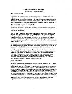
Prototyping and the Spiral Model of Development A software prototype is a working subset of a software system. Prototypes help check software designs and user interfaces, demonstrate key features to customers, or prove the feasibility of a proposed solution. A prototype may generate customer feedback on missing functionality, provide insight on how to improve the design, lead to a decision about whether to go ahead with a project or not, or form a starting point for the algorithms and data structures that will go into the final product. Prototyping is done early in the software development process. It fits naturally into the spiral model of development proposed by Barry Boehm (1988). Figure I-1 shows the spiral model; time is measured by the distance 1
2
PREFACE TO THE SECOND EDITION
from the center. Analysis, design, coding, and evaluation are repeated to produce a better product with each iteration. ”Prototyping” is the act of coding during those iterations when the software is not yet fully specified or the program does not yet remotely implement the required functionality.
Figure I-1 The Spiral Model of Software Development Tight spirals are better than loose spirals. The more powerful the prototyping tools, the less time and money spent in early iterations of development. This translates into either faster time to market, or a higher quality product. Some prototypes are thrown away once they have served the purpose of clarifying requirements or demonstrating some technique. This is OK, but in the spiral model some prototypes are gradually enhanced until they become the final production system.
Icon: a Very High Level Language for Applications Icon is a programming language developed at the University of Arizona. Icon generalizes its developers’ experience creating an earlier language, SNOBOL4. Icon embodies seminal research ideas, but it is also more fun and easier to program than other languages. Most very high-level languages revel in cryptic syntax, while Icon is not just more powerful, but often more readable than its competitors. This gain in expressive power without losing readability is an addicting result of Icon’s elegant design. The current Arizona Icon, version 9.5, is described in The Icon Programming Language, 3rd edition by Ralph and Madge Griswold (1996). Its reference implementation is a virtual machine interpreter. Icon evolved through many releases over two decades and is far more capable than it was originally. It is apparently a finished work.
Enter Unicon: More Icon than Icon The name “Unicon” refers to the descendant of Icon described in this book and distributed from www.unicon.org. Unicon is Icon with portable, platform-independent access to hard-
3 ware and software features that have become ubiquitous in modern applications development, such as objects, networks, and databases. Unicon is created from the same public domain source code that Arizona Icon uses, so it has a high degree of compatibility. We were not free to call it version 10 of the Icon language, since it was not produced or endorsed by the Icon Project at the University of Arizona. Just as the name Unicon frees the Icon Project of all responsibility for our efforts, it frees us from the requirement of backward compatibility. While Unicon is almost entirely backward compatible with Icon, dropping full compatibility allows us to clear out some dead wood and more importantly, to make some improvements in the operators that will benefit everyone at the expense of...no one but the compatibility police. This book covers the features of Icon and Unicon together. A compatibility check list and description of the differences between Icon and Unicon are given in Appendix D.
The Programming Languages Food Chain It is interesting to compare Icon and Unicon with the competition. Mainstream programming languages such as C, C++, and Java, like the assembler languages that were mainstream before them, are ideal tools for writing all sorts of programs, so long as vast amounts of programmer time are available. Throwing more programmers at a big project does not work well, and programmers are getting more expensive while computing resources continue to become cheaper. These pressures inexorably lead to the use of higher-level languages and the development of better design and development methods. Such human changes are incredibly slow compared to technological changes, but they are visibly occurring nevertheless. Today, the most productive programmers are using extra CPU cycles and memory to reduce the time it takes to develop useful programs. There is a subcategory of mainstream languages, marketed as rapid application development languages, whose stated goals seem to address this phenomenon. Languages such as Visual Basic or PowerBuilder provide graphical interface builders and integrated database connectivity, giving productivity increases in the domain of data entry and presentation. The value added in these products are in their programming environments, not their languages. The integrated development environments and tools provided with these languages are to be acclaimed and emulated, but they do not provide productivity gains that are equally relevant to all application domains. They are only a partial solution to the needs of complex applications. Icon is designed to be easier and faster to program than mainstream languages. The value it adds is in the expressive power of the language itself, in the category of very high level languages that includes Lisp, APL, Smalltalk, REXX, Perl, Tcl, Python, and Ruby; there are many others. Very high-level languages can be subdivided into scripting languages and applications languages. Scripting languages often glue programs together from disparate sources. They are typically strong in areas such as multilingual interfacing and file
4
PREFACE TO THE SECOND EDITION
system interactions, while suffering from weaker expression semantics, typing, scope rules, and control structures than their applications-oriented cousins. Applications languages typically originate within a particular application domain and support that domain with special syntax, control structures, and data types. Since scripting is an application domain, scripting languages are just one prominent subcategory of very high-level languages. Icon is an applications language with roots in text processing and linguistics. Icon programs tend to be more readable than similar programs written in other very high-level languages, making Icon well-suited to the aims of literate programming. For example, Icon was used to implement Norman Ramsey’s literate programming tool noweb (Ramsey, 1994). Literate programming is the practice of writing programs and their supporting textual description together in a single document. Unicon makes the core contributions of Icon useful for a broader range of applications. This book’s many examples illustrate the range of tasks for which Unicon is well suited, and these examples are the evidence in support of Unicon’s existence. Consider using Unicon when one or more of the following conditions are true. The more conditions that are true, the more you will benefit from Unicon. • Programmer time must be minimized. • Maintainable, concise source code is desired. • The program includes complex data structures or experimental algorithms. • The program involves a mixture of text processing and analysis, custom graphics, data manipulation, network or file system operations. • The program must run on several operating systems and have a nearly identical graphical user interface with little or no source code differences. Unicon is not the last word in programming. You probably should not use Unicon if your program has one or more of the following requirements: • The fastest possible performance is needed. • The program has hard real-time constraints. • The program must perform low-level or platform-specific interactions with the hardware or operating system. Programming languages play a key role in software development. The Unicon language is a very high level object-oriented language with a unique combination of expressive power and scalable rapid development. In this book, many examples from a wide range of application areas demonstrate how to apply and combine Unicon’s language constructs to solve realworld problems. It is time to move past the introductions. Prepare to be spoiled by this language. You may have the same feelings that Europeans felt when they gave up using Roman numerals and switched to the Hindu-Arabic number system. “This multiplication stuff isn’t that hard anymore!”
Part I Core Unicon
5
Chapter 1 Programs and Expressions This chapter presents many of the key features of Unicon, starting with those it has in common with other popular languages. Detailed instructions show how to compile and run programs. Soon the examples introduce important ways in which Unicon is different from other languages. These differences are more than skin deep. If you dig deeply, you can find dozens of details where Unicon provides just the right blend of simplicity, flexibility, and power. After this chapter, you will know how to • edit, compile, and execute Unicon programs • use the basic types to perform calculations • identify expressions that can fail, or produce multiple results • control the flow of execution using conditionals, looping, and procedures
1.1
Your First Unicon Program
This section presents the nuts and bolts of writing and running an Unicon program, after which you will be able to try the code examples or write your own programs. Before you can run the examples here or in any subsequent chapter, you must install Unicon on your system. (See Appendix F for details on downloading and installing Unicon from the Unicon web site, http://unicon.org.) We are going to be very explicit here, and assume nothing about your background. If you are an experienced programmer, you will want to skim this section, and move on to the next section. If you are completely new to programming, have no fear. Unicon is pretty easy to learn. All programs consist of commands that use hardware to obtain or present information to users, and perform calculations that transform information into a more useful form. To program a computer you write a document containing instructions for the computer to carry out. In Unicon a list of instructions is called a procedure, and a program is a collection of one or more procedures. In larger programs, groups of related procedures are organized 7
8
CHAPTER 1. PROGRAMS AND EXPRESSIONS
into classes or packages; these features are presented in Part II of this book. Unicon programs are text files that may be composed using any text editor. For the purposes of demonstration this section describes how to use Ui, the program editor and integrated development tool that comes with Unicon. It is time to begin. Fire up Ui by typing ”ui” from the command line, or launching the menu item or icon labeled ”Unicon,” and type: procedure main() write("Hello, amigo!") end Your screen should look something like Figure 1-1. The large upper area of the window is the editing region where you type your program code. The lower area of the window is a status region in which the Ui program displays a message when a command completes successfully, or when your program has an error. Until you explicitly name your file something else, a new file has the name noname.icn. The font Ui uses to display source code is selectable from the Options menu.
Figure 1-1: Writing an Unicon program using the Ui program.
1.1. YOUR FIRST UNICON PROGRAM
9
The list of instructions that form a procedure begins with the word procedure and ends with the word end. Procedures have names. After writing a list of instructions in a procedure you may refer to it by name without writing out the list again. The write() instruction is just such a procedure, only it is already written for you; it is built in to the language. When you issue a write() instruction, you tell the computer what to write. The details a procedure uses in carrying out its instructions are given inside the parentheses following that procedure’s name; in this case, "Hello, amigo!" is to be written. When you see parentheses after a name in the middle of a list of instructions, it is an instruction to go execute that procedure’s instructions. Inside the parentheses there may be zero, one, or many values supplied to that procedure. Besides writing your program, there are a lot of menu commands that you can use to control the details of compiling and executing your program within Ui. For instance, if you select Run→Run, Ui will do the following things for you. 1. Save the program in a file on disk. All Unicon programs end in .icn; you could name it anything you wished, using the File→SaveAs command. 2. Compile the Unicon program from human-readable text to (virtual) machine language. To do this step manually, you can select the Compile→Make executable command. 3. Execute the program. This is the main purpose of the Run command. Ui performed the other steps in order to make this operation possible. If you type the hello.icn file correctly, the computer should chug and grind its teeth for awhile, and Hello, amigo! should appear in a window on your screen. This ought to be pretty intuitive, since the instructions included the line write("Hello, amigo!") in it. That’s how to write to the screen. It’s that simple. The first procedure to be executed when a program runs is called main(). Every instruction listed in the procedure named main() is executed in order, from top to bottom, after which the program terminates. Use the editor to add the following lines right after the line write("Hello, amigo") in the previous program: write("How are you?") write(7 + 12) The end result after making your changes should look like this:
10
CHAPTER 1. PROGRAMS AND EXPRESSIONS procedure main() write("Hello, amigo!") write("How are you?") write(7 + 12) end
Run the program again. This example shows you what a list of instructions looks like, as well as how easy it is to tell the computer to do some arithmetic. Note It would be fine (but not very useful) to tell the computer to add 7 and 12 without telling it to write the resulting value. On seeing the instruction 7 + 12 the computer would do the addition, throw the 19 away, and go on. Add the following line, and run it: write("7 + 12") This illustrates what quotes are for. Quoted text is taken literally; without quotes, the computer tries to simplify (do some arithmetic, or compute the value of what is written), which might be difficult if the material in question is not an expression! write(hey you) makes no sense and is an error. Add this line, and run it: write(7 + "12") The 12 in quotes is taken literally as some text, but that text happens to be digits that comprise a number, so adding it to another number makes perfect sense. The computer will not have as much success if you ask it to add 7 to “amigo”. The computer views all of this in terms of values. A value is a unit of information, such as a number. Anything enclosed in quotes is a single value. The procedure named write() prints values on your screen. Operators such as + take values and combine them to produce other values, if it is possible to do so. The values you give to + had better be numbers! If you try to add something that doesn’t make sense, the program will stop running at that point, and print an error message. By now you must have the impression that writing things on your screen is pretty easy. Reading the keyboard is just as easy, as illustrated by the following program: procedure main() write("Type a line ending with :") write("The line you typed was" , read()) end
1.1. YOUR FIRST UNICON PROGRAM
11
Run the program to see what it does. The procedure named read() is used to get what the user types. It is built in to the language. The read() instruction needs no directions to do its business, so nothing is inside the parentheses. When the program is run, read() grabs a line from the keyboard, turns it into a value, and produces that value for use in the program, in this case for the enclosing write() instruction. The write() instruction is happy to print out more than one value on a line, separated by commas. When you run the program, the "the line you typed was" part does not get printed until after you type the line for read() and that instruction completes. The write() instruction must have all of its directions (the values inside the parentheses) before it can go about its business. Now let’s try some variations. Can you guess what the following line will print? write("this line says " , "read()") The read() procedure is never executed because it is quoted! Quotes say ”take these letters literally, not as an equation or instruction to evaluate.” How about: write("this line says , read()") Here the quotes enclose one big value, which is printed, comma and all. The directions one gives to a procedure are parameters; when you give a procedure more than one parameter, separated by commas, you are giving it a parameter list. For example, write("this value ", "and this one") Compile and run the following strange-looking program. What do you think it does? procedure main() while write( "" ˜== read() ) end This program copies the lines you type until you type an empty line by pressing Enter without typing any characters first. The "" are used just as usual. They direct the program to take whatever is quoted literally, and this time it means literally nothing - an empty line. The operator ˜== stands for ”not equals”. It compares the value on its left to the value on its right, and if they are not equal, it produces the value on the right side; if they are equal, it fails - that is, the “not equals” operator produces no value. If you have programmed in other languages, this may seem like a strange way to describe what is usually performed with nice simple Boolean values True and False. For now, try to take this description at face value; Unicon has no Boolean type or integer equivalent, it uses a more powerful concept that we will examine more fully in the chapters that follow. Thus, the whole expression "" ˜== read() takes a line from the keyboard, and if it is not empty, it produces that value for the enclosing write() instruction. When you type an empty
12
CHAPTER 1. PROGRAMS AND EXPRESSIONS
line, the value read() produces is equal to "", and ˜== produces no value for the enclosing write() instruction, which similarly fails when given no value. The while instruction is a ”loop” that repeats the instruction that follows it until that instruction fails (in this case, until there is no more input). There are other kinds of loops, as well as another way to use while; they are all described later in this chapter. So far we’ve painted you a picture of the Unicon language in very broad strokes, and informally introduced several relevant programming concepts along the way. These concepts are presented more thoroughly and in their proper contexts in the next sections and subsequent chapters. Hopefully you are already on your way to becoming an Icon programmer extraordinaire. Now it is time to dive into many of the nuts and bolts that make programming in Unicon a unique experience.
1.2
Command Line Options
Unicon comes with an IDE, but you can edit programs with any editor, and compile and run them from your operating system’s command line. This section describes the Unicon command line tools along with several useful options. The Unicon compiler executable is named unicon, and to compile the program foo.icn you would type unicon foo To execute the resulting program, just type foo To compile and link a program consisting of several modules, you can type them all on the command line, as in unicon foo bar baz but often you will want to compile them separately (using the -c command line option) and link the resulting object files, called ucode files; their extension is .u unicon -c foo unicon -c bar unicon -c baz unicon foo.u bar.u baz.u Some of the other useful command line options include: • -o arg
name the resulting output file arg
• -x args execute the program immediately after linking; this option goes after the program filenames
1.3. EXPRESSIONS AND TYPES • -t
turn on tracing
• -u
produce a warning for undeclared variables
13
These options can be specified in the Ui program under the Compile menu’s Compile Options command. Other options exist; consult your Unicon and Icon manual pages and platform-specific help files and release information for more details.
1.3
Expressions and Types
Each procedure in a Unicon program is a sequence of expressions. Expressions are instructions for obtaining values of some type, such as a number or a word; some expressions also cause side effects, such as sending data to a hardware device. Simple expressions just read or write a value stored in memory. More interesting expressions specify a computation that manipulates zero or more argument values to obtain result values by some combination of operators, procedures, or control structures. The simplest expressions are literal s, such as 2 or "hello, world!". These expressions directly specify a value stored in memory. When the program runs, they do not do any computation, but rather evaluate to themselves. Literals are combined with other values to produce interesting results. Each literal has a corresponding type. This chapter focuses on the atomic types. Atomic types represent individual, immutable values. The atomic types in Unicon are integer and real (floating-point) numbers, string (a sequence of characters), and cset (a character set). Atomic types are distinguished by the fact that they have literal values, specified directly in the program code and represented as data in the compiled code. Values of other types such as lists are constructed during execution. Later chapters describe structure types that organize collections of values, and system types for interacting with the operating system via files, databases, windows, and network connections. After literals, references to variables are the next simplest form of expression. Variables are named memory locations that hold values for use in subsequent expressions. You refer to a variable by its name, which must start with a letter or underscore and may contain any number of letters, underscores, or numbers. Use names that make the meaning of the program clear. The values stored in variables are manipulated by using variable names in expressions like i+j. This expression results in a value that is the sum of the values in the variables i and j, just like you would expect. Some words may not be used as variable names because they have a special meaning in the language. These reserved words include procedure, end, while, and so on. Other special variables called keywords start with the ampersand character (&) and denote special values. For example, global variables are initialized to the null value represented by the keyword &null. Other keywords include &date, &time, and so on. Complete lists of reserved words and keywords are given in Appendix A.
14
CHAPTER 1. PROGRAMS AND EXPRESSIONS
Unlike many languages where you have to state up front (declare) all the variables you are going to use and specify their data type, in Unicon variables do not have to be declared at all, and any variable can hold any type of value. However, Unicon will not allow you to mix incompatible types in an expression. Unicon is type safe, meaning that every operator checks its argument values to make sure they are compatible, converts them if necessary, and halts execution if they cannot be converted.
1.4
Numeric Computation
Unicon supports the usual arithmetic operators on data types integer and real. Integers are signed whole numbers of arbitrary magnitude. The real type is a signed floating point decimal number whose size on any platform is the largest size supported by machine instructions, typically 64-bit double precision values. In addition to addition (+), subtraction (-), multiplication (*) and division (/), there are operators for modulo (%) and exponentiation (ˆ). Arithmetic operators require numeric operands. Note Operations on integers produce integers; fractions are truncated, so 8/3 produces 2. If either operand is a real, the other is converted to real and the result is real, so 8.0/3 is 2.66666... As a general rule in Unicon, arguments to numeric operators and functions are automatically converted to numbers if possible, and a run-time error occurs otherwise. The built-in functions integer(x) and real(x) provide an explicit conversion mechanism that fails if x cannot be converted to numeric value, allowing a program to check values without resulting in a run-time error. In addition to the operators, built-in functions support several common numeric operations. The sqrt(x) function produces the square root of x, and exp(x) raises e to the x power. The value of pi (3.141...) is available in keyword &pi, the Golden Ratio (1.618...) is available in &phi, and e (2.718...) is available in &e. The log(x) function produces the natural log of x. The common trigonometric functions, such as sin() and cos() take their angle arguments in radian units. The min(x1, x2, ...) and max(x1, x2, ...) routines return minimum and maximum values from any number of arguments. Appendix A gives a complete list of built-in functions and operators. Listing 1-1 shows a simple Unicon program that illustrates the use of variables in a numeric computation. The line at the beginning is a comment for the human reader. Comments begin with the # character and extend to the end of the line on which they appear. The compiler ignores them. Listing 1-1 Mystery program # What do I compute? procedure main()
1.5. STRINGS AND CSETS
15
local i, j, old_r, r i := read() j := read() old_r := r := min(i, j) while r > 0 do { old_r := r if i > j then i := r := i % j else j := r := j % i } write(old_r) end This example illustrates assignment; values are assigned to (or ”stored in”) variables with the := operator. As you saw in the previous section, the function read() reads a line from the input and returns its value. The modulo operator (%) is an important part of this program: i % j is the remainder when i is divided by j. While loops can use a reserved word do followed by an expression (often a compound expression in curly braces). The expression following the do is executed once each time the expression that controls the while succeeds. Inside the while loop, a conditional if-then-else expression is used to select from two possible actions. The names of the variables in this example are obscure, and there are no comments in it other than the one at the top. Can you guess what this program does, without running it? If you give up, try running it with a few pairs of positive numbers. In addition to arithmetic operators, there are augmented assignment operators. To increment the value in a variable by 2, these two statements are equivalent: i +:= 2 i := i + 2 Augmented assignment works for most binary operators, not just arithmetic. The expression i op:= expr means the same as i := i op expr.
1.5
Strings and Csets
The non-numeric atomic types in Unicon are character sequences (strings) and character sets (csets). Icon came from the domain of string processing, and from it Unicon inherits many sophisticated features for manipulating strings and performing pattern matching. This section presents the simple and most common operations. More advanced operations and examples using strings and csets are given in Chapter 4.
16
CHAPTER 1. PROGRAMS AND EXPRESSIONS
String literals are enclosed in double quotes, as in "this is a string", while cset literals are enclosed in single quotes, as in ’aeiou’. Although strings and csets are composed of characters, there is no character type; a string (or cset) consisting of a single character is used instead. Current implementations of Unicon use eight-bit characters, allowing strings and csets to be composed from 256 unique characters. ASCII representation is used for the lower 128 characters, except on EBCDIC systems. The appearance of non-ASCII values is platform dependent. Like integers, strings can be arbitrarily large, constrained only by the amount of memory you have on your system. Several operators take string arguments. The *s operator gives the length of string s. The expression s1||s2 produces a string consisting of the characters in s1 followed by s2. The subscript operator s[i] produces a one-letter substring of s at the ith position. Indices are counted starting from position 1. If i is nonpositive, it is from the end of the string, for example s[-2] is the second to the last character in the string. Csets support set operators. c1++c2 produces a cset that is the union of c1 and c2. The expression c1**c2 is the intersection, while c1--c2 is the difference. In addition, several keywords are commonly used csets. The keywords &letters, &lcase, and &ucase denote the alphabetic characters, lower case characters a-z, and upper case characters A-Z, respectively, while &digits is the set from 0-9, &ascii is the lower 128 characters, and &cset is the set of all (256, on most implementations) characters. Many built-in functions operate on strings and csets. Some of the simple string functions are reverse(s), which produces a string that is the reverse of s, and trim(s,c), which produces a substring of s that does not end with any character in cset c. Functions and operators that require string arguments convert numeric values to strings automatically, and halt execution with a run-time error if given a value that cannot be converted to a string.
1.6
Goal-directed Evaluation
So far, the examples of how expressions are evaluated have included nothing you wouldn’t find in ordinary programming languages. It is time to push past the ordinary. In most conventional languages, each expression always computes exactly one result. If no valid result is possible, a sentinel value such as -1, NULL, EOF (end-of-file) or INF (infinity) is returned instead. This means that the program must check the return value for this condition. For example, while reading integers from the input and performing some operation on them you might do something like this: while (i := read()) ˜= -1 do process(i)
1.6. GOAL-DIRECTED EVALUATION
17
This will work, of course, except when you really need to use -1 as a value! It is somewhat cumbersome, however, even when a sentinel value is not a problem. Unicon provides a much nicer way to write this type of code, developed originally in the Icon language. In Unicon, expressions are goal-directed. This means that every expression when evaluated has a goal of producing results for the surrounding expression. If an expression succeeds in producing a result, the surrounding expression executes as intended, but if an expression cannot produce a result, it is said to fail and the surrounding expression cannot be performed and in turn fails. Now take a look at that loop again. If it weren’t for the termination condition, you would not need the intermediate variable i. If you would like to say: process(read()) your wishes are answered by Unicon; you can indeed write your program like this. The expression read() tries to produce a value by reading the input. When it is successful, process() is called with the value; but when read() cannot get any more values, that is, at the end of the file, it fails. This failure propagates to the surrounding expression and process() is not called either. Here is the clincher: control expressions like if and while don’t check for Boolean (true/false) values, they check for success! So our loop becomes while process(read()) The do clause of a while loop is optional; in this case, the condition does everything we need, and no do clause is necessary. Consider the if statement that was used in the earlier arithmetic example: if i > j then ... Comparison operators such as > succeed or fail depending on the values of the operands. This leads to another question: if an expression like i < 3 succeeds, what value should it produce? No ”true” value is needed, because any result other than failure is interpreted as ”true.” This allows the operator to return a useful value instead! The comparison operators produce the value of their right operand when they succeed. You can write conditions like if 3 < i < 7 then ... that appear routinely in math classes. Other programming languages only dream about being this elegant. First, Unicon computes 3 < i. If that is true, it returns the value i, which is now checked with 7. This expression in fact does exactly what you’d expect. It checks to see that the value of i is between 3 and 7. (Also, notice that if the first comparison fails, the second one will not be evaluated.)
18
CHAPTER 1. PROGRAMS AND EXPRESSIONS
1.7
Fallible Expressions
Because some expressions in Unicon can fail to produce a result, you should learn to recognize such expressions on sight. These fallible expressions control the flow of execution through any piece of Unicon code you see. When failure is expected it is elegant. When it is unexpected in your program code, it can be disastrous, causing incorrect output that you may not notice or, if you are lucky, the program may terminate with a run-time error. Some fallible expressions fail when they cannot perform the required computation; others are predicates whose purpose is to fail if a condition is not satisfied. The subscript and sectioning operators are examples of the first category. The expression x[i] is a subscript operator that selects element i out of some string or structure x. It fails if the index i is out of range. Similarly, the sectioning operator x[i:j] fails if either i or j are out of range. The read() function is illustrative of a large number of built-in functions that can fail. A call to read() fails at the end of a file. You can easily write procedures that behave similarly, failing when they cannot perform the computation that is asked. Unfortunately, for an arbitrary procedure call p(), you can’t tell if it is fallible without studying its source code or reference documentation. The safest thing is to expect any procedure call is fallible and check whether it failed, unless you know it is not fallible or its failure doesn’t matter. Following this advice may avoid many errors and save you lots of time. In this book we will be careful to point out fallible expressions when we introduce them. The less than operator < is a typical predicate operator, one that either fails or produces exactly one result. The unary predicates /x and \x test a single operand, succeeding and producing the operand if it is null, or non-null, respectively. The following binary predicates compare two operands. The next section presents some additional, more complex fallible expressions. < >= = ˜= numeric comparison operators >= == ˜== lexical (alphabetic) comparison === ˜=== reference comparison
1.8
Generators
So far we have seen that an expression can produce no result (failure) or one result (success). In general, an expression can produce any number of results: 0, 1, or many. Expressions that can produce more than one result are called generators. Consider the task of searching for a substring within a string: find("lu", "Honolulu") In most languages, this would return one of the substring matches, usually the first position at which the substring is found. In Unicon, this expression is a generator, and
1.8. GENERATORS
19
can produce all the positions where the substring occurs. If the surrounding expression only needs one value, as in the case of an if test or an assignment, only the first value of a generator is produced. If a generator is part of a more complex expression, then the return values are produced in sequence until the whole expression produces a value. Let us look at this example: 3 < find("or", "horror") The first value produced by find() is 2, which causes the < operation to fail. Execution then resumes the call to find(), which produces a 5 as its next value, and the expression succeeds. The value of the expression is the first position of the substring greater than 3. The most obvious generator is the alternation operator |. The expression expr1 | expr2 produces its left-hand side followed by its right-hand side, if needed by the surrounding expression. This can perform many computations quite compactly. For example, x = (3 | 5) checks to see if the value of x is 3 or 5. More complex expressions follow logically: (x | y) = (3 | 5) checks to see if either x or y has the value 3 or 5. It is the Unicon equivalent of C’s (x == 3) || (x == 5) || (y == 3) || (y == 5) In understanding Unicon code, it helps if you identify the generators, if there are any. In addition to the alternation operator | and the function find(), there are a few other generators in Icon’s built in repertoire of operators and functions. We mention them briefly here, so you can be on the lookout for them when reading code examples. The expression i to j is a generator that produces all the values between i and j. The expression i to j by k works similarly, incrementing each result by k; i, j, and k must all be integer or real numbers, and k must be non-zero. The expression i to j is equivalent to i to j by 1. The unary ! operator is a generator that produces the elements of its argument. This works on every type where it makes sense. Applied to a string, it produces all its characters (in order). Sets, tables, lists, or records produce the members of the structure. Generators get resumed for more results as needed in order for the surrounding expression to succeed, and this may propagate through many levels of nested enclosing expressions. However, special expressions called bounded expressions will never resume their generator subexpressions. For example, the conditional expressions used in if and while are never resumed if they succeed; if they produce a result the then-branch or the loop body is executed, and if that code fails, it does not cause generators in the conditional to be resumed.
20
CHAPTER 1. PROGRAMS AND EXPRESSIONS
Those bounded conditional expressions are re-evaluated starting from scratch if execution comes their way again. Another popular bounded expression is the semi-colon operator. The expression expr1 ; expr2 evaluates the two expressions in order, and bounds the first expression, so you don’t have to worry about backtracking into it if the second expression fails.
1.9
Iteration and Control Structures
You have already seen two control structures in Unicon: the if and the while loop, which test for success. Unicon has several other control structures that vary in complexity and usefulness. Unicon is expression-based, and all control structures are expressions that can be used in surrounding expressions if desired. The big difference between control structures and ordinary operators or procedures is that ordinary operators and procedures don’t execute until their arguments have been evaluated and produced a result; they don’t execute at all if an argument fails. In contrast, a control structure uses one of its arguments to decide whether (or how many times) to evaluate its other arguments. Since control structures are expressions, they may produce a result for a surrounding expression. For example, the result of an if expression is the result of either its then part or its else part, whichever one was selected. On the other hand, a loop executes until its test fails, after which there is no meaningful result for it to produce; loops usually fail as far as surrounding expressions are concerned. The control structure every processes the entire sequence of values produced by a generator. The expression every expr1 do expr2 evaluates expr2 for each result generated by expr1. This loop looks similar enough to a while loop to confuse people at first. The difference is that a while loop re-evaluates expr1 from scratch after each iteration of expr2, but every resumes expr1 for an additional result where it left off the last time through the loop. Using a generator to control a while loop makes no sense; the generator will restart each iteration, which may give you an infinite loop. Similarly, not using a generator to control an every loop also makes no sense; if expr1 is not a generator the loop body executes at most one time. The classic example of every is a loop that generates the number sequence from a to expression, assigning the number to a variable that can be used in expr2. In many languages these are called “for” loops. A for loop in Unicon is written like this: every i := 1 to 10 do write(i) Of course, every and to are not limited to this BASIC-style for loop. Generators are more flexible; the for loop above looks clumsy when compared with the equivalent
1.9. ITERATION AND CONTROL STRUCTURES
21
every write(1 to 10) A generator operand to a non-generator forms a generator. The enclosing non-generator (such as write()) is re-run each time the generator suspends and resumes. Unicon’s every keyword generalizes the concept of iterators found in other languages. Iterators are special control structures that walk through a collection of data. Instead of being a special feature, in Unicon iterators are just one of many ways to utilize generators. The sequence of results from an expression does not have to be stored in a structure to iterate over them. The sequence of results does not even have to be finite; many generator expressions produce an infinite sequence of results, as long as the surrounding expression keeps asking them for more. Here is another example of how every expressions are more flexible than for loops. The expression every f(1 | 4 | 9 | 16 | 25 | 36) executes the function f several times, passing the first few square numbers as parameters. A shorter equivalent that uses the power operator (ˆ) is every f((1 to 6)ˆ2). An example in the next section shows how to generalize this to work with all the squares. The if, while, and every expressions are Unicon’s primary control structures. Several other control structures are available that may be more useful in certain situations. The loop until expr1 do expr2 is while’s evil twin, executing expr2 as long as expr1 fails; on the other hand repeat expr is an infinite loop, executing expr over and over. There are also variations on the if expression introduced earlier for conditional execution. First, the else branch is optional, so you can have an if expression that does nothing if the condition is not satisfied. Second, there is a special control structure introduced for the common situation in which several alternatives might be selected using a long sequence of if ... else if ... else if ... expressions. The case expression replaces these chains of if expressions with the syntax: case expr of { branch1: expr1 branch2: expr2 ... default: expr i }
22
CHAPTER 1. PROGRAMS AND EXPRESSIONS
When a case expression executes, the expr is evaluated, and compared to each branch value until one that matches exactly is found, as in the binary equality operator ===. Branch expressions can be generators, in which case every result from the branch is compared with expr . The default branch may be omitted in case expressions for which no action is to be taken if no branch is satisfied. When we introduced the repeat loop, you probably were wondering how to exit from the loop, since most applications do not run forever. One answer would be to call one of the built-in functions that terminate the entire program when it is time to get out of the loop. The exit(), stop(), and runerr() functions all serve this valuable purpose; their differences are described in Appendix A. A less drastic way to get out of any loop is to use the break expression: break expr This expression exits the nearest enclosing loop; expr is evaluated outside the loop and treated as the value produced by executing the loop. This value is rarely used by the surrounding expression, but the mechanism is very useful, since it allows you to chain any number of breaks together, to exit several levels of loops simultaneously. The break expression has a cousin called next that does not get out of a loop, but instead skips the rest of the current iteration of a loop and begins the next iteration of the loop.
1.10
Procedures
Procedures are a basic building block in most languages. Here is an example of an ordinary procedure. This one computes a simple polynomial, ax2 + bx + c. procedure poly(x,a,b,c) return a * xˆ2 + b * x + c end
Parameters Procedure parameters are passed by value except for structured data types, which are passed by reference. This means that when you pass in a string, number, or cset value, the procedure gets a copy of that value; any changes the procedure makes to its copy will not be reflected in the calling procedure. On the other hand, structures that contain other values, such as lists, tables, records, and sets are not copied. The procedure being called gets a handle to the original value, and any changes it makes to the value will be visible to the calling procedure. Structure types are described in the next chapter. When you call a procedure with too many parameters, the extras are discarded. This feature is valuable for prototyping but can be dangerous if you aren’t careful! Similarly, if
1.10. PROCEDURES
23
you call a procedure with too few parameters, the remaining variables are assigned the null value, &null. The null value is also passed as a parameter if you omit a parameter. Now it is time to describe the unary operators \ and /. These operators test the expression against the null value. The expression /x succeeds and returns x if the value is the null value. This can be used to assign default values to procedure arguments: Any arguments that have a null value can be tested for and assigned a value. Here’s an example: procedure succ(x, i) /i := 1 return x + i end If this procedure is called as succ(10), the missing second parameter, i, is assigned the null value. The forward slash operator then tests i against the null value, which succeeds; therefore the value 1 is assigned to i. The backward slash checks if its argument is non-null. For example, this will write the value of x if it has a non-null value: write("The value of x is ", \x) If x does in fact have the null value, then \x will fail, which will mean that the write() procedure will not be called. If it helps you to not get these two mixed up, a slash pushes its operand ”up” for non-null, and ”down” for a null value. The procedure succ() shows one way to specify a default value for a parameter. The built-in functions use such default values systematically to reduce the number of parameters needed; consistent defaults for entire families of functions make them easy to remember. Another key aspect of the built-in operations is implicit type conversion. Arguments to built-in functions and operators are converted as needed. Defaulting and type conversion are so common and so valuable in Unicon that they have their own syntax. Parameter names may optionally be followed by a coercion function (usually the name of a built in type) and/or a default value, separated by colons. These constructs are especially useful in enforcing the public interfaces of library routines that will be used by many people. procedure succ(x:integer, i:integer:1) end This parameter declaration is a more concise equivalent of procedure succ(x, i) x := integer(x) | runerr(101, x) /i := 1 | i := integer(i) | runerr(101, i) end
24
CHAPTER 1. PROGRAMS AND EXPRESSIONS
Variables and scopes Variable names used as parameters are fundamentally different from procedure names. The scope of parameters is limited to the body of a single procedure, while procedure names are visible to the entire program. Parameters and procedures are special forms of two basic kinds of variables in Unicon: local variables and global variables. The scope of global variables, including procedure names, consists of the entire program. Their value is stored in memory for the entire execution of the program. There are two kinds of local variables; both introduce names that are defined only within a particular procedure. Regular local variables are created when a procedure is called, and destroyed when a procedure fails or returns a result; a separate copy of regular local variables is created for each call. Static local variables are global variables whose names are visible only within a particular procedure; a single location in memory is shared by all calls to the procedure, and the last value assigned in one call is remembered in the next call. Variables do not have to be declared, and by default they are local. To get a global variable, you have to declare it outside any procedure with a declaration like this: global MyGlobal Such a declaration can be before, after, or in between procedures within a program source file, but cannot be inside a procedure body. Of course, another way to declare a global variable is to define a procedure; this creates a global variable initialized with the appropriate procedure value containing the procedure’s instructions. Regular and static local variables may be declared at the top of a procedure body, after the parameters and before the code starts, as in the following example: procedure foo() local x, y static z ... end Each declared local variable name may be followed by a := and an initializer expression that specifies the variable’s initial value. Without an initializer, variables start with the value &null. Although you do not have to declare local variables, large programs, library code or multi-person projects should declare all local variables. If you don’t, and some other part of the code introduces a global variable by the same name as your undeclared local, your variable will be interpreted as a reference to the global. To help avoid this problem, the -u command line option to the compiler causes undeclared local variables to produce a compilation error message. A procedure body can begin with an initial clause, which executes only the first time the procedure is called. The initial clause is mainly used to initialize static variables in ways
1.10. PROCEDURES
25
that aren’t handled by initializers. For example, the following procedure returns the next number in the Fibonacci sequence each time it is called, using static variables to remember previous results in the sequence between calls. procedure fib() static x,y local z initial { x := 0 y := 1 return 1 } z := x + y x := y y := z return z end
Writing your own generators When a procedure returns a value, the procedure and its regular local variables cease to exist. But there are expressions that don’t disappear when they produce a value: generators! You can create your own generators by writing procedures that use suspend instead of return. suspend is different from return in that it saves the point of execution within the procedure; if another value is required by the calling expression, the generator continues execution from where it previously left off. Here is a procedure to generate all the squares. Instead of using multiplication, it uses addition to demonstrate generators! The code uses the fact that if we keep adding successive odd numbers, we get the squares. procedure squares() odds := 1 sum := 0 repeat { suspend sum sum +:= odds odds +:= 2 } end To perform a computation on the squares, we can use it in an every statement: every munge(squares())
26
CHAPTER 1. PROGRAMS AND EXPRESSIONS
Warning This is an infinite loop! (Do you know why? Whether munge() succeeds or fails, every will always resume squares() for another result to try; squares() generates an infinite result sequence.) The fail expression makes the procedure fail. Control goes to the calling procedure, returning no value, and the procedure call ceases to exist; it cannot be resumed. A procedure also fails implicitly when control flows off the end of the procedure’s body. Here is a procedure that produces all the non-blank characters of a string, but bails out if the character # is reached: procedure nonblank(s) every c := !s do { if c == "#" then fail if c ˜== " " then suspend c } end
Recursion A recursive procedure is one that calls itself, directly or indirectly. There are many cases where it is the most natural way of solving the problem. Consider the famous ”Towers of Hanoi” problem. Legend has it that when the universe was created, a group of monks in a temple in some remote place were presented with a problem. There are three diamond needles, and on one of them is a stack of 64 golden disks all of different sizes, placed in order with the largest one at the bottom and the smallest on top. All the disks are to be moved to a different needle under the conditions that only one disk may be moved at a time, and a larger disk can never be placed on a smaller disk. When the monks finish this task, the universe will come to an end. How can you move the n smallest disks? If n is 1, just move it. Since it’s the smallest, this will not violate the condition. If n is greater than 1, here’s what we can do: first, move the n-1 upper disks to the intermediate needle, then transfer the nth disk, then move the n-1 upper disks to the destination needle. This whole procedure does not violate the requirements either (satisfy yourself that such is the case). Now write the procedure hanoi(n) that computes this algorithm. The first part is simple: if you have one disk, just move it. procedure hanoi(n, needle1:1, needle2:2) if n = 1 then write("Move disk from ", needle1, " to ", needle2) Otherwise, perform a recursive call with n-1. First, to find the spare needle we have: other := 6 - needle1 - needle2
1.10. PROCEDURES
27
Now move the n-1 disks from needle1 to other, move the biggest disk, and then move the n-1 again. The needles are passed as additional parameters into the recursive calls. They are always two distinct values out of the set {1, 2, 3}. hanoi(n-1, needle1, other) write("Move disk from ", needle1, " to ", needle2) hanoi(n-1, other, needle2) That’s it! You’re done. Listing 1-2 contains the complete program for you to try: Listing 1-2 Towers of Hanoi procedure main() write("How many disks are on the towers of Hanoi?") hanoi(read()) end procedure hanoi(n:integer, needle1:1, needle2:2) local other if n = 1 then write("Move disk from ", needle1, " to ", needle2) else { other := 6 - needle1 - needle2 hanoi(n-1, needle1, other) write("Move disk from ", needle1, " to ", needle2) hanoi(n-1, other, needle2) } end Turn on tracing see how this program works. To enable tracing, compile your program with a -t option, or assign the keyword &trace a non-zero number giving the depth of calls to trace. Setting &trace to -1 will turn on tracing to an infinite depth. To move n disks, 2 n - 1 individual disk movements will be required. If the monks move one disk a second, it will take 2 64 - 1 seconds, or about 60 trillion years. Wikipedia has listed the age of the universe at around 13.75 billion years. It seems unlikely that we need worry about the monks finishing their task!
Summary In this chapter you have learned: • Unicon is an expression-based language organized as a set of procedures starting from a procedure called main(). • Unicon has four atomic types: arbitrary precision integers, real numbers, arbitrary length strings of characters, and character sets.
28
CHAPTER 1. PROGRAMS AND EXPRESSIONS • There is no Boolean concept in Unicon; instead, control is driven by whether an expression succeeds in producing a result or fails to do so. This eliminates the need for most sentinel values, shortening many expressions. • Generator expressions can produce multiple results as needed by the surrounding expression in order for it to produce results. • Procedure parameters are passed by value for atomic types, and by reference for all other data types. Unicon features extensive argument defaults and automatic type coercion throughout its built-in function and operator repertoire. • Unicon has two scope levels: global and local. Undeclared variables are implicitly defined to be local.
Chapter 2 Structures The examples in the previous chapter employed data types whose values are immutable. For example, all operations that manipulate numbers and strings compute new values, rather than modify existing values. This chapter presents structured types that organize and store collections of arbitrary (and possibly mixed) types of values. When you complete this chapter, you will understand how to use these types. • Tables associate their elements with key values for rapid lookup. • Lists offer efficient access by position as well as by stack or queue operations. • Records store values using a fixed number of named fields. • Sets support operations such as union and intersection on groups of elements. • Using structures to represent trees, graphs, and matrices. There are several structure types that describe different basic relationships between values. The philosophy of structures in Unicon is to provide built-in operators and functions for common organization and access patterns - the flexible ”super glue” that is needed by nearly all applications. Their functionality is similar to the C++ Standard Template Library or generic classes in other languages, but Unicon’s structure types are much simpler to learn and use, and are well supported by the expression evaluation mechanism described in the previous chapter. All structure types in Icon share many aspects in common, such as the fact that structures are mutable. The values inside them may change. In that respect, structures are similar to a collection of variables that are bundled together. In many cases, Unicon’s structure types are almost interchangeable! Operators like subscripts and built-in functions such as insert() are defined consistently for many types. Code that relies on such operators is polymorphic: it may be used with multiple structure types in an interchangeable way. For both the structures described in this chapter and the strings described in the next chapter, be aware that Unicon performs automatic storage management, also known as 29
30
CHAPTER 2. STRUCTURES
garbage collection. If you have used a language like C or C++, you know that one of the biggest headaches in writing programs in these languages is tracking down bugs caused by memory allocation, especially dynamic heap memory allocation. Unicon transparently takes care of those issues for you. Another big source of bugs in languages like C and C++ are pointers, values that contain raw memory addresses. Used properly, pointers are powerful and efficient. The problem is that they are easy to use incorrectly by accident; this is true for students and practicing software engineers alike. It is easy in C to point at something that is off-limits, or to trash some data through a pointer of the wrong type. Unicon has no pointer types, but all structure values implicitly use pointer semantics. A reference is a pointer for which type information is maintained and safety is strictly enforced. All structure values are references to data that is allocated elsewhere, in a memory region known as the heap. You can think of a reference as a safe pointer: the only operations it supports are copying the pointer, or dereferencing it using an operation that is defined for its type. Assigning a structure to a variable, or passing it as a parameter, gives that variable or parameter a copy of the reference to the structure but does not make a copy of the structure. If you want a copy of a structure, you call the function copy(x), which makes a “shallow” copy of a single table, list, record, or set. If that structure contains references to other structures as its elements, those substructures are not copied by copy(). To copy a “deep” structure (lists of lists, tables of records, etc.) you can use the procedure deepcopy() that is given as an example later in this chapter.
2.1
Tables
Tables are unordered collections of values that are accessed using associated keys. They are Unicon’s most versatile type. All of the other structure types can be viewed as special cases of tables, optimized for performance on common operations. Most operations that are defined for tables are defined for other structure types as well. Subscripts are used for the primary operations of associating keys with values that are inserted into the table, and then using keys to look up objects in the table. The table() function creates a new empty table. For example, the lines T := table() T["hello"] := "goodbye" create a new table, and associate the key "hello" with the value "goodbye". The table() function takes one optional argument: the default value to return when lookup fails. The default value of the default value is &null, so after the above example, write(T["goodbye"]) would write an empty line, since write() treats a null argument the same as an empty string, and write() always writes a newline. Assigning a value to a key that is not in the table
2.2. LISTS
31
inserts a value into the table. This occurs in the second line of the example above, so write(T["hello"]) writes out "goodbye". Subscripts are the primary operation on tables, but there are several other useful operations. The insert(T, k1 , x1 , k2 , x2 , ...) function adds new key-value pairs to T. The delete(T, k1 , k2 , ...) function deletes values from T that correspond to the supplied keys. Icon’s unary * operator produces the size of its argument; for a table, *T is the number of key-value pairs in the table. Unary ! generates elements from a collection; for a table, !T generates the values stored in the table. Unary ? is the random operator; for a table, ?T produces a random value stored in the table. Both unary ! and ? produce values stored in a table, not the keys used to lookup values. Function member(T, k) succeeds if k is a key in T and fails otherwise. Function key(T) generates the keys that have associated values. The following example prints word counts for the input (assuming getword() generates words of interest): wordcount := table(0) every word := getword() do wordcount[word] +:= 1 every word := key(wordcount) do write(word, " ", wordcount[word]) The default value for the table is 0. When a new word is inserted, the default value gets incremented and the new value (that is, 1) is stored with the new word. Tables grow automatically as new elements are inserted.
2.2
Lists
Lists are dynamically sized ordered collections of values. They are accessed by subscripts, with indexes starting at 1. You can also insert or remove elements from the beginning, middle, or end of the list. Lists take the place of arrays, stacks, queues, and deques found in other languages and data structures textbooks. A list is created by calling the function list(), which takes optional parameters for the lists’s initial size and the initial value given to all elements of the list. By default list() creates an empty list. Alternatively, you can create a list by enclosing a comma-separated sequence of values in square brackets: L := ["linux", 2.0, "unix"] Lists are dynamic. Lists grow or shrink as a result of stack and queue operations. The push() and pop() functions add and remove elements from the front of a list, while put() and pull() add and remove elements at the end of the list. In addition, insert(L, i, x) inserts x at position i, and delete(L, i) deletes the element at position i. The expression [] is another way to create an empty list; it is equivalent to calling list() with no arguments. The previous list could have been constructed one element at a time with the following code. put() accepts a variable number of arguments.
32
CHAPTER 2. STRUCTURES L := [ ] put(L, "linux") put(L, 2.0) put(L, "unix")
Elements of the list can be obtained either through list manipulation functions or by subscripting. Given the list L above, in the following code the first line writes "unix" while the second line moves the first element to the end of the list. write(L[3]) put(L, pop(L)) There is no restriction on the kinds of values that may be stored in a list. For example, the elements of a list can themselves be lists. You can create lists like L := [[1, 2, 3], [4, 5, 6], [7, 8, 9]] and index them with multiple subscripts. L[2][3] is equivalent to L[2,3] and yields the value 6 in this example. Lists also support several common operators. The operator *L produces the size of list L. The operators !L and ?L generate the elements of L in sequence, and produce a single random element of L, respectively. The following procedure uses the unary ! operator to sum the values in list L, which must be numbers. procedure sum(L) total := 0 every total +:= !L return total end Comparing the two, lists are like tables with boring keys: the positive integers starting from 1. Function member(L, k) succeeds if 0 < integer(k) " || \(p.symlink) return s end The record returned by stat() contains many fields. Not all file systems support all of these fields. Two of the most important portable fields are size, the file size in bytes, and mtime, the file’s last modified time, an integer that is converted into a human readable string format by ctime(i). Another important field is mode, a string that indicates the file’s type and access permissions. Its first letter (mode[1]) is "-" for normal files, "d" for directories, and some file systems support additional types. The other characters of the mode string are platform dependent. On UNIX there are nine letters to encode read, write, and execute permissions for user, group, and world, in the format: "rwxrwxrwx". On a classic Windows FAT file system, there is only "rwa" to indicate the status of hidden, read-only, and archive bits (if it is set, the system bit is indicated in mode[1]). Some file systems support duplicate directory entries called links that refer to the same file. In the record returned by stat(), a link is indicated by a mode[1] value of "l". In addition, field nlinks (”number of links”) will be > 1 and/or field symlink may be the string filename of which this file is an alias. Appendix E includes information on each platform’s support for the mode field, as well as stat()’s other fields.
Controlling file ownership and access The previous section shows how different platforms’ file systems vary in their support for the concepts of file ownership and access. If the system supports ownership, the user and
5.3. PROGRAMS AND PROCESS CONTROL
69
group that own a file are changed by calling chown(fname, user, group). The chown() function only succeeds for certain users, such as the super user. User and group may be string names, or integer user identity codes on some platforms. File access rights are changed with chmod(fname, mode). The chmod() function only succeeds for the owner of a given file. The mode is a nine-letter string similar to stat()’s mode field, or an octal encoding of that information (see Appendix E). Another piece of information about files is called the umask. This is a variable that tells the system what access rights any newly created files or directories should have. The function call umask("rwxr-xr-x") tells the system that newly created directories should have a permission of "rwxr-xr-x" and files should have permissions of "rw-r--r--". The mkdir(s, mode) function takes an optional mode parameter, which can override the umask for for newly created directories. Ordinary files are never given execute permission by the system, it must be set explicitly with chmod().
File locks Files can be locked while a program is updating some information. If the contents of the file are in an inconsistent state, other programs may be prevented from reading (or especially writing) the file. Programs can cooperate by using file locks: flock(filename, "x") The first call to flock() creates a lock, and subsequent calls by other programs will block, waiting till the writing program releases its lock. The flag "x" represents an exclusive lock, which should be used while writing; this means no other process can be granted a lock. For reading, "s" should be used to create a shared lock so that other programs that are also just reading can do so. In this way you can enforce the behavior that only one process may open the file for writing, and all others will be locked out; but many processes can concurrently open the file for reading.
5.3
Programs and Process Control
Unicon’s system interface is similar but higher level than the POSIX C interface. An include file posix.icn defines constants used by some functions. Include files are special code, consisting mainly of defined symbols, intended to be textually copied into other code files. They are handled by the preprocessor, described in Appendix A. To include posix.icn in a program, add this line at the top of your program: $include "posix.icn" When a system call fails, the integer keyword &errno indicates the error that occurred. As seen earlier, a human-readable string is also available in &errortext. Error codes (such
70
CHAPTER 5. THE SYSTEM INTERFACE
as EPERM, or EPIPE) are defined in posix.icn; &errno can be compared against constants like ENOENT. In general, however, human readers will prefer to decipher &errortext. In the discussion to follow, a program is the code, while a process is such a program in execution. This distinction is not usually important, but for network applications it matters, since the same program can run in multiple processes, and a process can change the program that it is running.
Signals A signal is an asynchronous message sent to a process either by the system (usually as a result of an illegal operation like a floating point error) or by another process. A program has two options to deal with a signal: it can allow the system to handle it in the default manner (which may include termination of the process) or it can register a function, called a signal handler, to be run when that signal is delivered. Signals are trapped or ignored with the trap(s, p) function. Argument s is the string name of the signal. The signal names vary by platform; see Appendix E. You can trap any signal on any machine; if it is not defined it will be ignored. For example, Linux systems don’t have a SIGLOST. Trapping that signal has no effect when a program runs on Linux. The trap() function’s second argument is the procedure to call when the signal is received. The previous signal handler is returned from trap() so it can be restored by a subsequent call to trap(). The signal handler defaults to the default provided by the system. For instance, SIGHUP is ignored by default but SIGFPE will cause the program to terminate. Here is an example that handles a SIGFPE (floating point exception) by printing out a message and then runs the system default handler:
global oldhandler ... trap("SIGFPE", sig_ignore) oldhandler := signal("SIGSEGV", handler) ... # restore the old handler trap("SIGSEGV", oldhandler) end procedure sig_ignore(s); end procedure handler(s) write(&errout, "Got signal ", s) (\oldhandler)(s) # propagate the signal end
5.3. PROGRAMS AND PROCESS CONTROL
71
Launching programs Many applications execute other programs and read their results. In many cases, the best way to do this is to call open() with mode "p" (pipe) to launch a command. In mode "p" the string argument to open() is not a filename, it is an entire command string. Piped commands opened for reading (mode "p" or "pr") let your program read the command’s standard output, while piped commands open for writing (mode "pw") allow your program to write to the command’s standard input. The more general function system(x,f1,f2,f3,mode) runs an external command (argument x) with several options. If x is a list, x[1] is the command to execute and the remaining list elements are its command line arguments. If x is a string, it is parsed into arguments separated by spaces. Arguments with spaces in them may be escaped using double quotes. A program that calls system() normally waits for the launched program to complete before continuing, and system() returns the integer status of the completed command. If s ends in an ampersand (&) or the optional mode argument is 1 or "nowait", system() does not wait for the command to complete, but instead launches the command in the background and returns an integer process id. The system() function takes three optional file arguments that specify redirected standard input, output, and error files for the launched program.
Using file redirection and pipes One common scenario is for a program to run another program but with the input and output redirected to files. On command-line systems like the Unix shells or the MS-DOS command prompt, you may have used redirection: prog < file1 File redirection characters and other platform-dependent operations are supported in the command string passed to system(), as in the following system() call: system("prog < file1") Pipes to and from the current program are nicely handled by the open() function, but sometimes the input of one program needs to be connected to the output of another program. You may have seen uses like this: prog1 | prog2 The pipe() function returns a pair of open files in a list, with the property that anything written to the second file will appear on the first. Here’s how to hook up a pipe between two programs:
72
CHAPTER 5. THE SYSTEM INTERFACE L := pipe() | stop("Couldn’t get pipe: ", &errortext) system("prog1 &", , L[2]) system("prog2 &", L[1]) close(L[1]) close(L[2])
Process information The integer process identity can be obtained with getpid(). The user id of the process can be obtained with getuid() if the platform supports it. Calls to obtain additional information such as group identity on some platforms are described in Appendix E. A parent process may want to be notified when any of its children quit (or change status). This status can be obtained with the function wait(). When a child process changes state from “running” to either “exited” or “terminated” (and optionally “stopped”), wait() returns a string of the form pid:status:arg:core The ":core" will only be present if the system created a core file for the process. The status can be any of “exited”, “terminated” or “stopped”. The arg field is either: a) the exit status of the program if it exited; or b) the signal name if it was terminated. Typically wait() will be used in the handler for the SIGCHLD signal which is sent to a process when any of its children changes state. The arguments to wait() are the pid of the process to wait for and any options. The default for pid is to wait for all children. The options may be either "n", meaning wait() should not wait for children to block but should return immediately with any status that’s available, or "u", meaning that any processes that stopped should also be reported. These options may be combined by using "nu".
The select() system call Some programs need to be able to read data from more than one source. For example, a program may have to handle network traffic and also respond to the keyboard. The problem with using read() is that if no input is available, the program will block and will not be able to handle the other stream that may in fact have input waiting on it. To handle this situation, you can use the function select(x1,x2,...i). The select() function tells the system which files you are interested in reading from, and when input becomes available on any of those sources, the program will be notified. The select() function takes files or lists of files as its arguments, and returns a list of all files on which input is waiting. If an integer argument is supplied, it is a timeout that gives the maximum milliseconds to wait before input is available. If the timeout expires, an empty list is returned. If no timeout is given, the program waits indefinitely for input on one of the files.
5.4. NETWORKING
73
while *(L := select(f1, f2, f3, timeout)) = 0 do handle_timeout() (&errno = 0) | stop("Select failed: ", &errortext) every f := !L do { # Dispatch reads pending on f ... } When using select() to process input from multiple files, you may need to pay some attention to avoid blocking on any one of your files. For example the function read() waits until an entire line has been typed and then returns the whole line. Consider this code, which waits for input from either a file (or network connection) or a window designated by keyword &window: while L := select(f, &window) do if !L === f then c := read(f) Just because select() has returned doesn’t mean an entire line is available; select() only guarantees that at least one character is available. The command shell log application in Chapter 14 shows the usage of select(). Another primary application area for select() is network programming, described later in this chapter. For network connections, the function reads(f, i) will return as soon as it has some input characters available, rather than waiting for its maximum string size of i. But if no input is available, reads() blocks.
Non-blocking input and the ready() function The function ready(f, i) is like reads(f, i) except that it is non-blocking, that is, it returns immediately with up to i bytes if they are available, but it does not wait around. It is ideal for use with select() and in situations where a server or client needs to interact with multiple remote connections.
5.4
Networking
Unicon provides a very high-level interface to Internet communications. Applications with custom communications use one of the major Internet applications protocols, TCP and UDP. An higher level interface to several popular Internet protocols such as HTTP and POP is provided by means of Unicon’s messaging facilities.
TCP A TCP connection is a lot like a phone call: to make a connection you need to know the address of the other end, just like a phone number. For TCP, you need to know the name of
74
CHAPTER 5. THE SYSTEM INTERFACE
the machine to connect to, and an address on that machine, called a port. A server listens for connections to a port; a client sends requests to a port. Also, there are two kinds of ports, called ”Internet Domain” and ”Unix Domain.” The distinction is beyond the scope of this book; we will just mention that Internet Domain ports are numbers, and Unix Domain ports look like files. Also, a connection to a Unix domain port can only be made from the same machine, so we will not consider the Unix domain further here. A call to open() with mode "n" (network) requests a network connection. The first argument to open() is the network address, a host:port pair for Internet domain connections, and a filename for Unix domain sockets. If the address contains no host name and therefore starts with ":", the socket is opened on the same machine. The value returned by open() is a file that can be used in select() and related system functions, as well as normal reading and writing. A client uses mode "n" with open() to open a connection to a TCP server. Here is a simple version of the Internet ”finger” program: procedure main(argv) local fserv := getserv("finger") | stop("Couldn’t get service: ", &errortext) name := argv[1] host := "" argv[1] ? { name := tab(find("@")) & ="@" & host := tab(0) } if *host > 0 then write("[", host, "]") f := open(host || ":" || fserv.port, "n") | stop("Couldn’t open connection: ", &errortext) write(f, name) | stop("Couldn’t write: ", &errortext) while write(read(f)) end Notice the use of getserv(). The posix_servent record it returns includes fields for the name, aliases, port, and protocol used by the Internet service indicated in getserv()’s argument. The Internet protocols specify the ports to be used for various services; for instance, email uses port 25. Instead of having to remember port numbers or hard-coding them in our program, we can just use the name of the service and have getserv() translate that into the port number and protocol we need to use. To write a server, all we need to do is add "a" (accept) to the mode after the "n" in open(). Here is a simple TCP server that listens on port 1888: procedure main() while f := open(":1888", "na") do { system("myserverd -servicerequest &", f, f)
5.4. NETWORKING
75
close(f) } (&errno = 0) | stop("Open failed: ", &errortext) end The call open(":1888", "na") blocks until a client connects. The returned value is a file that represents the network connection. This example server responds to requests by launching a separate process to handle each request. The network connection is passed to myserverd as its standard input and output, so that process had better be expecting a socket on its standard I/O files, and handle it appropriately. This works on UNIX; on other platforms a different approach is needed. Launching a separate process to handle requests is standard operating procedure for many Internet servers, but besides the portability concerns, it uses a lot of memory and CPU time. Many servers can be implemented in a single process. Chapter 15 includes an example of such a server. Mode "na" is less than ideal for one-process servers: it only supports one connection at a time. When waiting for a new connection, the process is not doing any computation, and when servicing a connection, the program is not listening for any other connection requests. Unless each connection is of short duration, the server will appear to be down, or appear to be unacceptably slow, to anyone trying to connect while an existing request is being processed.
Determining IP numbers Many programs need the IP number of the machine they are talking to. Given a network connection f, image(f) will show the IP address and port of the client machine that is connected (this is sometimes called the peername). Some programs need to know their own IP number, but each machine can have several IP numbers, one for each kind of physical network hardware in operation. To obtain a list of local IP numbers, a program can read the output of /sbin/ifconfig (UNIX) or ipconfig (Windows). To find the IP number used for a particular network connection n, on some platforms you can call gethost(n), which returns a string with the IP number and port used by the local machine for a given connection. If you do determine your IP number in one of these ways, it is usually not the number seen by the world, because most devices are connecting through some form of network address translation. To see the number that the world sees, you have to connect to someone else and ask them to tell you what IP number they see you at. procedure main(argv) n := open(argv[1],"n") | stop("can’t connect to ", argv[1]|"missing host") write("connected to: ", image(n)[6:-1]) write("using: ", gethost(n))
76
CHAPTER 5. THE SYSTEM INTERFACE end
Non-blocking network opens Servers need to never block. The call open(":port","nl") creates a listener on the specified port, without waiting around for someone to actually connect to it. The network file returned from open() is not open for reading or writing, so it is not good for much...yet. About the only thing you can do with such a file is include it (along with any other network connections you have going) as an argument in a call to select(). If a listener matches a current connection request, select() converts it into a regular network connection as per mode "na". In addition to non-blocking servers’ listener connections, in the real-world clients need a way to do an almost non-blocking connection as well. TCP connections over long distances take a highly variable amount of time, but most clients do not want to “freeze” for a couple of minutes while the connection attempt times out. The network client versions of open() allows an optional third parameter to supply it with a timeout value, in milliseconds.
UDP UDP is another protocol used on the Internet. TCP is like a phone call: all messages you send on the connection are guaranteed to arrive in the same order they were sent. UDP on the other hand is more like the postal service, where messages are not guaranteed to reach their destination and may not arrive in the same order they were sent in. Messages sent via UDP are called datagrams. It’s a lot cheaper (faster) to send UDP messages than TCP, though, especially if you are sending them across the Internet rather than to a local machine. Sending a postcard is usually cheaper than a long distance phone call! UDP datagrams can be sent either with an open()/writes() pair, or with send(). Typically a server sends/receives on the same socket so it will use open() with read() and write(). A client that only sends one or two datagrams uses send()/receive(). The following example provides a service called ”rdate” that allows a program to ask a remote host what time it has. The server waits for request datagrams and replies with the date and time. The "u" flag added to the mode in the call to open() signifies that a UDP connection should be used. The function receive() waits for a datagram to arrive, and then it constructs a record having the address the message came from and the message in it. The server uses the address to send the reply. f := open(":1025", "nua") while r := receive(f) do { # Process the request in r.msg ... send(r.addr, reply) }
5.5. MESSAGING FACILITIES
77
The record returned by receive() has two fields: the addr field contains the address of the sender in "host:port" form, and the msg field contains the message. To write a UDP client, use mode "nu" Since UDP is not reliable, the receive() is guarded with a select(); otherwise, the program might hang forever if the reply is lost. The timeout of five seconds in the call to select() is arbitrary and might not be long enough on a congested network or to access a very remote host. Notice the second argument to getserv(); it restricts the search for Internet service information to a particular network protocol, in this case UDP. procedure main(args) (*args = 1) | stop("Usage: rdate host") host := args[1] s := getserv("daytime", "udp") f := open(host||":"||s.port, "nu") | stop("Open failed: ", &errortext) writes(f, " ") if *select(f, 5000) = 0 then stop("Connection timed out.") r := receive(f) write("Time on ", host, " is ", r.msg) end From these examples you can see that it is relatively easy to write programs that use Internet communication. But TCP and UDP are very general, somewhat low-level protocols; most programs employ a higher-level communication protocol, either by defining their own, or using a standard protocol. If you need to define your own Internet protocol, you can do it on top of TCP or UDP; if your program needs to use a standard Internet protocol, you should check first to see if the protocol is built-in to the language as part of the messaging facilities, described in the next section.
5.5
Messaging Facilities
Unicon’s messaging facilities provide higher level access to many popular Internet protocols. A call to open() using mode "m" establishes a messaging connection. The filename argument to a messaging connection is a URI (Uniform Resource Indicator) that specifies the protocol, host machine, and resource to read or write. The protocols implemented thusfar are HTTP, Finger, SMTP, and POP. Extra arguments to open() are used to send headers defined by the protocol. For example, the call open("mailto:unicon-group", "m", "Reply To:
[email protected]") supplies a Reply To field as a third parameter to open() on an SMTP connection. Header fields from the server’s response to a connection are read by subscripting the message connection value with a string header name; an example is in the next section.
78
CHAPTER 5. THE SYSTEM INTERFACE
HTTP HTTP is used to read or write to Web servers; the content read or written typically consists of HTML text. The following program, httpget.icn, fetches a remote file specified by a URI on the command line, and saves it as a local file. The Icon Program Library module basename is used to extract the filename from the URI. link basename procedure main(argv) f1 := open(argv[1],"m") f2 := open(basename(argv[1]),"w") while write(f2, read(f1)) end This example retrieves the actual data for a successful HTTP request; for a failed request the connection returns no data, appearing to be an empty file. Programs can check the HTTP status code in order to determine the nature of the problem. Status codes and other metadata from HTTP header lines are inspected by subscripting the connection with the desired header. For example, in the previous program, checking f1["Status-Code"] would allow us to detect HTTP errors, and f1["Location"] would allow us to find the new location of the file, if the HTTP server had informed us that the file had moved. You can retrieve this status information on a remote file without retrieving the file itself. If you open a URI with mode "ms" instead of "m", an HTTP request for header information is made, but no data is retrieved.
SMTP and POP SMTP is used to send a mail message. Mail is delivered via an SMTP server machine on which the user must have a valid account. These default to the current user on the current host machine. Two environment variables UNICON SMTPSERVER and UNICON USERADDRESS can be set to override the default behavior. POP is used to read mail messages. POP is the least file-like of these protocols. A POP connection feels like a list of strings, each string containing an entire mail message, rather than a simple sequence of bytes. Function read() and operator ! produce entire messages which in general contain many newline characters. POP messages may be removed by either delete() or pop(); messages are buffered in such a way that message removal on the server occurs when the connection is explicitly and successfully closed. Here’s a simple program that illustrates the use of msesaging to get email from a POP server. It gets messages from the server without deleting them and, for every message, prints out who the message is from as well as the subject line.
5.6. TASKS
79
procedure main(argv) user := argv[1] | getenv("USER") | stop("no user") passwd := argv[2] | getenv("PASSWD") | stop("no password") server := argv[3] | getenv("MAILHOST") | "mailhost" conn := open("pop://"||user||":"||passwd||"@"||server, "m") | stop("couldn’t connect to the POP server ", server) every msg := !conn do msg ? while line := tab(find("\n")) do if =("From: " | "Subject: ") then write(line) close(conn) end You should improve the password handling in this program if you use it! Chapter 14 includes another example use of Unicon’s POP messaging facilities: a spam filter.
5.6
Tasks
A task is an executing program within the Unicon virtual machine. A single task called the root is created when the interpreter starts execution. Additional tasks are created dynamically as needed. The tasking facilities allow Unicon programs to load, execute, communicate with, and control one another, all within a single instantiation of the Unicon interpreter. Although Unicon programs can use the tasking facilities to load and execute any number of other programs within the same interpreter space, the tasking facilities do not introduce a concurrent programming construct nor do they include special support for multiprocessor hardware. Their domain is that of high-level language support for programs that benefit from or require a tighter coupling than that provided by inter-process communication; that is, programs that access each other’s state extensively. Co-expressions provide the tasking facilities’ program execution model, and coexpression activation serves as the communication mechanism. The extensions are general enough to be useful in a wide variety of contexts. For example, programs that use the multi-tasking interface can communicate directly without resorting to external files or pipes. At the language level, the tasking facilities include several built-in functions and keywords, but no new types, declarations, or control structures. Several existing functions have been extended to offer additional support for the multi-tasking environment. Separate memory allocation regions are established for each task.
Preliminary terminology Before describing the task model, a few definitions are needed. These definitions pertain to regions of memory referenced by programs during execution.
80
CHAPTER 5. THE SYSTEM INTERFACE
A name space is a mapping from a set of program source-code identifiers to a set of associated memory locations [Abelson85]. Icon programs have a global name space shared across the entire program and various name spaces associated with procedures. Procedures each have a static name space consisting of memory locations shared by all invocations of the procedure and local name spaces private to each individual invocation of the procedure. When a co-expression is created, a new local name space is allocated for the currently executing procedure, and the current values of the local variables are copied into the new name space for subsequent use by the co-expression. An Icon program has an associated program state consisting of the memory associated with global and static name spaces, keywords, and dynamic memory regions. Similarly, a co-expression has an associated co-expression state consisting of an evaluation stack that contains the memory used to implement one or more local name spaces. Co-expressions in an Icon program share access to the program state and can use it to communicate.
Tasks as extended co-expressions A task consists of a main co-expression and zero or more child co-expressions that share a program state consisting of the global and static name spaces, keywords, and dynamic memory regions. At the source-language level, tasks are loaded, referenced, and activated solely in terms of one of their member co-expressions; the task itself is implicit. Coexpressions share access to the program state and can use it to communicate. Unicon provides the task model as a mechanism for multi-tasking, but does not predefine the policy; matters such as the scheduling algorithm used and whether multi-tasking is co-operative or pre-emptive are programmable at the user level in terms of co-expression activations.
Task creation A task can create other tasks. The function load(s, L, f1, f2, f3, i1, i2, i3) loads an icode file [Gris86] specified by the file name s, creates a task for it and returns a co-expression corresponding to the invocation of the procedure main(L) in the loaded icode file. L defaults to the empty list. Unlike conventional Icon command-line argument lists, the argument list passed to load() can contain values of any type, such as procedures, lists, and tables in the calling task. The task being loaded is termed the child task, while the task calling load() is termed the parent. The collection of all tasks forms a tree of parent-child relationships. f1, f2, and f3 are file arguments to use as &input, &output, and &error in the loaded task; &input, &output, and &error default to those of the loading task. i1, i2, and i3 are three integer arguments that supply initial region sizes for the task’s block, string,
5.6. TASKS
81
and stack memory areas, respectively. i1 and i2 default to 65000, while i3 defaults to 20000 (the defaults may be changed by the environment variables BLKSIZE, STRSIZE, and MSTKSIZE).
Running other programs A co-expression created by load() is activated like any other co-expression. When activated with the @ operator, the child task begins executing its main procedure. Unless it suspends or activates &source, the child task runs to completion, after which control is returned to the parent. Chapter 5 presents an alternative means of executing a child with which the parent retains control over the child as it executes. This default behavior is illustrated by the program seqload, which loads and executes each of its arguments (string names of executable Unicon programs) in turn. Each of the strings passed on the command line and extracted from the list using the element-generation operator, !) is passed in turn to load(), which reads the code for each argument and creates a task in which to execute the loaded program. The tasks are then executed one-by-one by the co-expression activation operator, @. There is nothing special about this example except the semantics of the load() function and the independent execution environment (separate global variables, heaps, and so forth), that load() provides to each task. # seqload.icn procedure main(arguments) every @load(!arguments) end For example, if three Icon programs whose executable files are named translate, assemble, and link are to be run in succession, the command seqload translate assemble link executes the three programs without reloading the interpreter for each program.
Data access Although tasks have separate program states, they reside in the same address space and can share data; values can be transmitted from task to task through main()’s argument list, through co-expression activation, or by use of event monitoring facilities described in Chapter 10. In the following pair of programs, the parent receives a list value from the child and writes its elements out in reverse order. # parent.icn procedure main() L := @ load("child")
82
CHAPTER 5. THE SYSTEM INTERFACE while write(pull(L)) end # child.icn procedure main() L := [ ] while put(L, read()) return L end
Access Through Task Argument Lists The following program takes its first argument to be an Icon program to load and execute as a child, sorts its remaining arguments, and supplies them to the child program as its command-line arguments (pop() and sort() are Icon built-in functions that extract the first list element and sort elements, respectively): procedure main(arguments) @load(pop(arguments), sort(arguments)) end Argument lists allow more sophisticated data transfers; the seqload example presented earlier can be extended to transmit arbitrary structures between programs using argument lists in the following manner. As in seqload, each string naming an executable Icon program is passed into load(), and the resulting task is activated to execute the program. In this case, however, any result that is returned by one of the programs is assigned to local variable L and passed to the next program in the list via the second argument to load(). # seqload2.icn procedure main(arguments) every program := !arguments do L := @load(program, L) end The net effect of seqload2.icn is similar to a UNIX pipe, with an important difference: Arbitrary Icon values can be passed from program to program through the argument lists. This capability is more interesting in substantial multipass tools such as compilers, where full data structures can be passed along from tool to tool instead of writing out text encodings of the structures to a file.
Inter-task Access Functions Several built-in functions provide inter-task access to program data. These functions are usable in any multi-task Unicon context, but are especially useful in program execution monitoring, discussed in Chapter 9.
5.6. TASKS
83
For example, the variable() function takes a co-expression value as an optional second argument denoting the task from which to fetch the named variable. variable(s, C) is useful for assigning to or reading from another task’s variables. In the following seqload example, the parent initializes each child’s Parent global variable (if there is one) to refer to the parent’s &main co-expression. A child task can then use Parent to determine whether it is being run standalone or under a parent task. The variable() function is useful in inspecting values, especially at intermediate points during the monitored execution of a TP. # seqload3.icn procedure main(arguments) every arg := !arguments do { Task := load(arg) variable("Parent", Task) := &main @Task } end In addition to extending existing functions for monitoring, several new functions have been added. The use of these monitoring functions are illustrated in many example monitors in Unicon’s ipl/mprogs directory. Some of the intertask access functions are listed in Figure 5-1. In these functions, parameter C refers to a co-expression that may be from a task other than the one being executed. Functions that generate values can produce more than one result from a given call. cofail(C) fieldnames(r) globalnames(C) keyword(s, C)
transmit failure to C. generate fieldnames of record r. generate the names of C’s global variables. produces keyword s in C. Keywords are special global variables that have special semantics in certain language facilities. localnames(C,i) generates the names of C’s local variables, i calls up from the current procedure call. paramnames(C,i) generates the names of C’s parameters. staticnames(C,i) generates the names of C’s static variables. structure(C) generates the values in C’s block region, or heap. The heap holds structure types such as lists and tables. variable(s,C,i) produces variable named s, interpreted i levels up within C’s procedure stack. Figure 5-1: Unicon interprogram access functions.
84
CHAPTER 5. THE SYSTEM INTERFACE
Shared icode libraries Programs that are written to take advantage of the multi-tasking environment gain in space efficiency and modularity. Code sharing is one natural way to achieve space efficiency in a collection of programs. Since procedures are first-class data values in Icon, code sharing can be implemented via data sharing. Programs executing in a single invocation of the interpreter can share code easily if the code is not required to produce side effects on global variables in the calling task’s program state. If side-effects to the calling task’s program state are required, the shared code must generally be written with care to explicitly reference the calling task’s state. Side effects in the client task can also be achieved through the parameters passed in and results obtained by calling the shared procedure.
Loading shared code Consider a collection of applications that make extensive use of procedures found in the Icon program library (IPL) [Griswold90c]. If those applications are run using MT Icon, the IPL routines need be loaded only once, after which they may be shared. In order to reference shared code from a loaded task, two additional considerations must be satisfied: the shared code must be loaded, and the client tasks must be able to dynamically link shared routines into their generated code. Both of these problems can be solved entirely at the source level: In order to introduce a shared Icon procedure into the name space, a global variable of the same name must be declared. Managing the loading of shared libraries is itself a natural task to assign to an Icon procedure that uses a table to map strings to the pointers to the procedures in question.
Code sharing example The following collection of three programs illustrate one schema that allows code sharing. Other conventions can certainly be devised, and much of the sharing infrastructure presented here can be automatically generated. Program calc.icn consists of a shared library procedure named calc() and a main procedure that exports a reference to calc() for sharing: # calc.icn procedure calc(args...) # code for calc # (may call other routines in calc.icn if there are any) end procedure main() # initialization code, if any return calc end
5.7. SUMMARY
85
Note that a module exporting shared procedures can also have global variables (possibly initialized from other command-line arguments). Shared modules can export other values besides procedures using the same mechanism. The parent task that loads the various shared library clients implements a procedural encapsulation (loadlib() in this example) of an Icon table to store references to shared routines. The parent passes this procedure to clients. Each client calls the procedure for each shared routine. Routines that are already loaded are returned to requesting tasks after a simple Icon table lookup. Whenever a routine is requested that has not been loaded, the load() function is called and the shared library activated. procedure main(arguments) @load("client",put(arguments,loadlib)) end procedure loadlib(s, C) static sharedlib initial sharedlib := table() sharedlib[s] := @load(s) variable(s, C) := sharedlib[s] end A client of calc declares a global variable named calc, and assigns its value after inspecting its argument list to find the shared library loader: global loadlib global calc procedure main(arguments) if /loadlib then stop("no shared libraries present") loadlib("calc", ¤t) # ... remainder of program may call shared calc end
Sharing procedure collections The primary deficiency of the previous example is that it requires one shared library procedure per Icon module, that is, separate compilation. In practice it is more convenient to have a collection of related procedures in a given Icon compilation unit. Shared libraries can employ such a mechanism by resorting to a simple database that maps procedure names to load modules.
5.7
Summary
Unicon’s system facilities provide a high-level interface to the common features of modern operating systems, such as directories and network connections. This interface is vital to
86
CHAPTER 5. THE SYSTEM INTERFACE
most programs, and it also presents the main portability challenges, since a Unicon design goal is for applications to require no source code changes and no conditional code needed to run on most operating systems. Of course some application domains such as system administration are inevitably platform dependent. There are two major areas of the system interface that are whole application domains extensive enough to warrant an entire chapter of their own: databases and graphics. Databases can be viewed as a hybrid of the file and directory system interface with some of the data structures described in Chapter 2. Since many databases are implemented using a client/server architecture, the database interface also includes aspects of networking. Databases are presented in the Chapter 6. Graphics is another crucial component of the system interface, rich enough to warrant special features built-in to the language, and deep enough to warrant an entire book. Like databases, graphics can be viewed as an extension of the file data type described in this chapter. Unicon’s powerful 2D and 3D graphics facilities are discussed in Chapter 7.
Chapter 6 Databases Databases are technically part of the system interface described in the last chapter, but they are an important application area in their own right. Different kinds of databases are appropriate in different situations depending on how much information is to be stored and what kinds of accesses to the information are supported. This chapter describes three kinds of databases for which Unicon provides direct support, enabling you to: • Read and write memory-based structures to data files. • Use DBM databases as a persistent table data type. • Manipulate SQL databases through the ODBC connection mechanism.
6.1
Language Support for Databases
Unicon provides transparent access to databases stored in local files and on remote servers. The term transparent means that the built-in functions and operators used to access information in a database are the same as those used to access information in the memory-based structures presented in Chapter 2. To do this, connections to databases are represented by new built-in types that are extensions of the file and table data types. Some people might prefer a different syntax for databases from what is used for data structures. A different syntax, such as one based purely on function calls, would be consonant with the difference in performance the programmer can expect to see when accessing data in files as opposed to memory-based data structures. However, the performance of operators already depends on the type of the operands. Consider the expression !x. If x is a structure, its elements are generated from memory, but if x is a file, !x reads and generates lines from the file. The goal for Unicon is to make databases just as easy to learn and use as the rest of the language, and to minimize the introduction of new concepts. The word “database” means different things to different people; for some, it is the short form of “relational database.” This chapter uses the term database to refer to any method 87
88
CHAPTER 6. DATABASES
of providing persistent structures that store information from one program run to the next. The operators used to access a database determine whether one element at a time is read or written, or whether many operations are buffered and sent to the database together.
6.2
Memory-based Databases
If the entire database fits in memory at once, you can achieve vast speedups by avoiding the disk as much as possible. For example, all queries to read the database can be performed from memory. The database may be modified in memory immediately, and updated on the disk later on. Memory-based databases are increasingly feasible as workstation main memories grow larger, they are an excellent choice for many applications. One way to implement a memory-based database is to build up your arbitrary structure in memory, and then use the Icon Program Library module xcodes to write them out and read them in. The xcodes procedures convert structures to a string format that can be written to a file, and convert such strings back into the corresponding structure. The following sequence saves the contents of structure db to a file named db.dat. db := table() db["Ralph"] := "800-USE-ICON" db["Ray"] := "800-4UN-ICON" dbf := open("db.dat","w") xencode(db, dbf) close(dbf) The converse operation, reading in a structure from a file is also simple: dbf := open("db.dat") db := xdecode(dbf) close(dbf) write(db["Ralph"]) This approach works great for databases that do not need to be written to disk on an ongoing basis and for which the queries can readily be expressed as operations on structure types. For example, a telephone rolodex application would be well-served by this type of database. The data fits comfortably in memory, updates often occur in batches, and simple queries (such as a student’s name) provide sufficient access to the data. The other two kinds of databases in this chapter use traditional database technologies to efficiently address situations where this type of database is inadequate.
6.3
DBM Databases
A classic database solution on the UNIX platform is provided by the DBM family of library functions. DBM stands for Data Base Manager, and the functions maintain an association
6.3. DBM DATABASES
89
between keys and values on disk, which is very similar to the table data type. DBM was eventually followed by compatible superset libraries called NDBM (New Data Base Manager) and GDBM (GNU Data Base Manager). Unicon uses GDBM on all platforms. DBM databases are accessed via the open() function using mode "d" to open a database for reading and writing, or mode "dr" for read-only access. Once opened, DBM databases resemble the table data type and are manipulated using table operations. For example, if d is a DBM file, d[s] performs a database insert/update or lookup, depending on whether the expression is assigned a new value, or dereferenced for its current value. Values can also be inserted into the database with insert(d, k, v) and read from it with fetch(d, k). delete(d, k) similarly deletes key k from the database. DBM databases are closed using the close() function. The following example program takes a database and a key on the command line, and writes out the value corresponding to that key. procedure main(args) d := open(args[1], "d") | stop("can’t open ", args[1]) write(d[args[2]]) end If you are wondering why the call to open() isn’t followed by a call to close(), you are right, it is proper to close files explicitly, although the system closes all files when the program terminates. How would you generalize this program to accept a third commandline argument, and insert the third argument (if it is present) into the database with the key given by the second argument? You might easily wind up with something like this: procedure main(args) d := open(args[1], "d") | stop("can’t open ", args[1]) d[args[2]] := args[3] write(d[args[2]]) close(d) end DBM databases are good for managing data sets with a simple organization, when the size of the database requires that you update the database a record at a time, instead of writing the entire data set. For example, if you wrote a Web browser, you might use a DBM database to store the user’s set of bookmarks to Web pages of interest. There is one basic limitation of DBM databases when compared with the table data type that you should know about. DBM databases are string-based. The keys and values you put in a DBM database get converted and written out as strings. This makes the semantics of DBM databases slightly different from tables. For example, a table can have two separate keys for the integer 1 and the string "1", but a DBM database will treat both keys as the string "1". This limitation on DBM databases also means that you cannot use structure types such as lists as keys or values in the database. If the type is not convertible
90
CHAPTER 6. DATABASES
to string, it won’t work. You can use the functions xencode() and xdecode(), described in the previous section, to manually convert between strings and structures for storage in a DBM database if you really need this capability.
6.4
SQL Databases
DBM is great for data that is organized around a single key, but it is inadequate for complex databases. The industry standard choice for enterprise-level data organization is the Structured Query Language (SQL). SQL is supported by every major database vendor. Unlike DBM, a SQL database can contain multiple tables, and those tables are accessed by walking through a set of results to a query, rather than by accessing individual elements directly. SQL is designed for industrial-strength relational databases.
The SQL language The SQL language was invented by IBM and based on relational database theory developed by E.F. Codd. A database is a collection of tables, and each table is a collection of rows. The rows in a table contain information of various types in a set of named columns. Rows and columns are similar to records and fields, except that they are logical structures and do not describe physical form or layout of the data. There is an ANSI standard definition of SQL, but many vendors provide extensions, and most vendors are also missing features from the ANSI standard. Unicon allows you to send any string you want to the SQL server, so you can write portable “vanilla SQL” or you can write vendor-specific SQL as needed. SQL was originally intended for text-based interactive sessions between humans and their databases. Nowadays, SQL is primarily used “under the covers” by database applications that accommodate novice users with a graphical interface that does not require any knowledge of SQL, while supporting a SQL “escape hatch” for advanced users who may wish to do custom queries. This duality is paralleled in the Unicon language by the fact that Unicon’s built-in database operators and functions duplicate a subset of the capabilities of SQL. There are two ways to do things: using Unicon operations or using SQL statements. SQL statements can be divided into several categories, the most prominent of which are data definition and data manipulation. When using SQL within a Unicon program, you build up string values containing SQL statements. In the following examples, the SQL is given unadorned by double quotes or other Unicon artifacts. New tables are created with a CREATE TABLE statement, such as create table addresses (name varchar(40), address varchar(40), phone varchar(15)) Tables have a primary key that must be unique among rows in the table. By default the primary key is the first one listed, so name is the primary key in table addresses above.
6.4. SQL DATABASES
91
SQL’s data manipulation operations include SELECT, INSERT, UPDATE, and DELETE. SELECT determines the data set being operated on, picking rows and columns that form some projection of the original table. SELECT also allows you to combine information from multiple tables using relational algebra operations. Most databases are long-lived and evolve to include more columns of information over time. SQL’s ability to select and operate on projections is an important feature, since code that works with a certain set of columns continues to work after the database is modified to include additional columns. INSERT, UPDATE, and DELETE all modify the table’s contents. INSERT adds new rows to a table. For example: insert into addresses (name, address, phone) values (’Nick K’, ’1 Evil Empire’, ’(123)456-7890’) insert into addresses (name, address, phone) values (’Vic T’, ’23 Frozen Glade’, ’(900)888-8888’) UPDATE and DELETE can modify or remove sets of rows that match a particular criterion, as in update addresses set address = ’666 RTH, Issaquah’ where name = ’Nick K’ delete from addresses where name = ’Vic T’ This section presented only a few aspects of the SQL language. For simple database tasks you can in fact ignore SQL and use the Unicon facilities described in the rest of this chapter. However, for more complex operations the best solution is to formulate some SQL commands to solve the problem. A full discussion of SQL is beyond the scope of this book. For more information on this topic you might want to read one of the following books: Ramez Elmasri and Shamkant Navanthe’s Fundamentals of Database Systems, C.J. Date and Hugh Darwen’s A Guide to the SQL Standard.
Database architectures and ODBC SQL databases are accessed through an underlying Open DataBase Connectivity (ODBC) transport mechanism. This mechanism allows the programmer to ignore the underlying architecture. Hiding this complexity from application programmers is important. The database architecture may vary from a single process accessing a local database, to client/server processes, to three or more tiers spanning multiple networks. Figure 6-1 illustrates the role played by ODBC in providing Unicon with database access in one- and two-tier configurations. While this chapter cannot present a complete guide to the construction of database systems, it provides concrete examples of writing Unicon client programs that access typical database servers.
92
CHAPTER 6. DATABASES
Figure 6-1: Unicon and ODBC hide underlying architecture from applications
To use Unicon’s SQL facilities, you must have several software components in place. First, you need a SQL server that supports ODBC. You can buy a commercial SQL server, or use a free server such as MySQL (www.mysql.com) or PostgreSQL (www.postgresql.org). Second, you need an account, password, and permissions on the SQL server in order to connect to it. The details are server-dependent and outside the scope of this book. Third, your client machine needs an ODBC driver manager, and an ODBC driver for your SQL server; these must be configured properly. The driver manager is a component that connects applications to various databases; ODBC drivers are dynamic link libraries that database vendors supply to talk to their database. Figure 6-2 shows database configuration for MySQL via the MyODBC GUI dialog box on Windows (left), and in a ∼/odbc.ini file on Linux (right). In both cases, configuration involves knowing the internet server name or IP address, the port, and the database to connect to. For that triplet, you get to define a name called a DSN or data source name, which is the name that Unicon will pass in to open(). In the Windows dialog, this name is a textfield explicitly named as a DSN, while in the Linux odbc.ini file, it is at the top, inside the square brackets. In both cases, there are a lot of additional options which are beyond the scope of this book. On Windows, each ODBC driver may have its own custom dialogs for configuration, while on Linux the odbc.ini file is more the property of the driver manager and is used to configure all the various drivers. As a fair warning, the details required in the dialogs or the exact syntax of the odbc.ini and its required entries for a given driver change slightly from time to time and are beyond the scope of this book. Consult current ODBC documentation for the driver manager on your platform and the specific database to which you are connecting.
6.4. SQL DATABASES
93
[phones] Driver = /usr/lib64/libmyodbc5.so Description = phone example Server = localhost Database = phonebook Port = 3306
Figure 6-2: Configuring ODBC on Windows (left) and Linux (right) Once you have the ODBC software set up, writing the Unicon client program to connect to your database is straightforward.
Opening a SQL database To connect to a SQL database, call open() with mode "o". This establishes a session with a data source. The filename argument to open() is the data source to which you are connecting; it is associated with a particular ODBC driver, remote database server machine or IP number, and port within the ODBC driver manager. Mode "o" is followed by additional string arguments to open(). The first is an optional default table name used in the various functions that take a table name. Generally the arguments must then include the user name and password to use in connecting to the specified data source. Here is an example that establishes a connection to a database: f := open("unicondb", "o", "scott", "tiger") The open() function returns a value that supports many of the operations of both a file and a table, or fails if the connection cannot be established. The underlying session information is shared by multiple calls to open() the same database. In addition to the network connection and SQL session information that is retained, each database file value maintains a current selection consisting of a set of rows corresponding to the current query,
94
CHAPTER 6. DATABASES
and a cursor position within that selection. When a database is first opened, the selection consists of a null set containing no rows and no columns.
Querying and modifying a SQL database Subsequent queries to the database can be made by calling sql(db, sqlcmd). The sql() function sets the current selection within the database and places the cursor at the beginning of the set of selected rows. For example, to obtain Vic T’s phone number you might say sql(f, "select phone from addresses where name=’Vic T’") Vic’s phone number is included if you use the original select * query, but the more specific your query, the less time and network bandwidth is wasted sending data that your client application must filter out. You should do as much work on the server (in SQL) as possible to make the client more efficient. Since the function sql() transmits arbitrary SQL statements to the server, it can be used for many operations besides changing the current selection. The sql() function returns a null value when there is no return value from the operation, such as a create table statement. Its return value can be of varying type for other kinds of queries, and it can fail, for example if the SQL string is malformed or requests an impossible operation.
Traversing the selected rows To walk through the rows of your current database selection, you call fetch(db). The value returned is a row that has many of the operations of a record or a table, namely field access and subscripting operators. For example, if fetch(db) returns a row containing columns Name, Address, and Phone, you can write row := fetch(db) write(row.Name) write(row["Address"]) Called with one argument, fetch(db) advances the cursor one position. With two arguments, fetch(db, col) produces a column from the current row without advancing the cursor.
A SQL example application A human resources database might include two tables. One table might maintain employee information, such as names, identification numbers, and phone numbers, while another table maintains entries about specific jobs held, including employee’s ID, the pay rate, a code indicating whether pay is hourly or salaried, and the job title. Note that the SQL is embedded within a string literal.
6.4. SQL DATABASES
95
sql(db, "create table employees (id varchar(11), name varchar(40), phone varchar(15))") sql(db, "create table jobs (id varchar(11), payrate integer, is_salaried char, title varchar(40))") Inserting rows into the database looks like sql("insert into employees (id, name, phone) values(32, ’Ray’, ’274-2977’)") Now, how can you print out the job title for any particular employee? If you have the employee’s identification number, the task is easy, but let’s say you just have their name. These are the kinds of jobs for which SQL was created. Information from the employees table is effortlessly cross-referenced with the jobs table by the following SQL. The string is long so it is split into two lines. A Unicon string literal spans multiple lines when the closing doublequote has not been found and the line ends with an underscore character. sql(db, "select name,title from employees,jobs _ where name=’Ray’ and employees.id = jobs.id") while write(fetch(db).Title)
SQL types and Unicon types SQL has many data types, most of which correspond to Unicon types. CHAR and VARCHAR correspond to Icon strings; INTEGER and SMALLINT correspond to integers; FLOAT and REAL correspond to reals, and so on. The philosophy is to convert between Icon and SQL seamlessly and with minimal changes to the data format, but you should be aware that these are not exact matches. For example, it is possible to define a FLOAT with more precision than an Icon real, and it is easy to produce an Icon string that is longer than the maximum allowed VARCHAR size on most SQL servers. Unicon programmers writing SQL clients must be aware of the limitations of the SQL implementations they use. Unicon has structure types for which there is no SQL equivalent. Values of these types cannot be inserted into a SQL database unless you explicitly convert them to a SQLcompatible type (usually a string) using a function such as xencode(). SQL also has types not found in Unicon such as bit strings, timestamps, and BLOBS; they are represented by strings, and strings are used to insert such values into SQL databases. Strings are also used to represent out-of-range values when reading SQL columns into Unicon.
More SQL database functions SQL databases are feature-rich enough to warrant a suite of functions in addition to those they share with other kinds of files and databases. These functions are described in detail in Appendix A, but some of them deserve special mention. The function dbtables(db)
96
CHAPTER 6. DATABASES
is useful to obtain a listing of the data sources available within a particular database. Function dbcolumns(db) provides detailed information about the current table that is useful in writing general tools for viewing or modifying arbitrary SQL databases. The functions dbproduct(db) and dbdriver(db) produce information about the DBMS on which db resides, and the ODBC driver software used in the connection. The function dblimits(db) produces the upper bounds for many DBMS system parameters, such as the maximum number of columns allowed in a table. These functions return their results as a record or list of records whose field names and descriptions are given in Appendix A.
6.5
Tips and Tricks for SQL Database Applications
In addition to the complexity of learning SQL itself, SQL database applications have a characteristic flavor which may or may not seem natural to the Unicon programmer.
Operating on large files Asking for 200MB of data in a remote SQL database is a good way to bring a computer to its knees. Some SQL operations are slow due to an inefficient query on the remote server, while others are slow because large amounts of data are transmitted over a limited network connection. For a fixed amount of data, operation time will vary radically depending on how it is organized; fewer, larger tuples are transmitted faster than many smaller tuples.
Use multiple connections to nest queries It is common to use more than one table at once. Some times this is using SQL’s JOIN operation, but sometimes it is not. If you try to nest a second query inside a first one, you will quickly find that on a given connection, only one SELECT and one row set is maintained at a time. The second SELECT replaces the first, so for example: db := open("mydsn", "o", ...) sql(db, “SELECT ...”) while r := fetch(db) do { sql(db, “SELECT ...”) while r2 := fetch(db) do write(r2.foo) } does not work. Within your operating system and database server’s limits, the easy solution is to open multiple connections to your database: db1 := open("mydsn", "o", ...) db2 := open("mydsn", "o", ...) sql(db, “SELECT ...”)
6.5. TIPS AND TRICKS FOR SQL DATABASE APPLICATIONS
97
while r := fetch(db) do { sql(db2, “SELECT ...”) while r2 := fetch(db2) do write(r2.foo) }
Dynamic records Rows are represented as a special kind of Unicon record whose fields are determined at run-time from the names of selected columns. Record types introduced at runtime are called dynamic records, and they are useful in other contexts besides databases. The function constructor(rname, field, field, ...) produces a procedure that constructs records named rname with the given fields. The field names can be arbitrary strings, but only legal identifiers will be subsequently accessible via the field operator (.)
The db library The declaration link db provides simplified SQL access routines for non-SQL programmers. This library will not allow you to avoid learning SQL for long, but may ease the conversion from Unicon structure values into SQL strings for transmission over the network. The most useful of these procedures is dbupdate(), which sends a record (tuple) to the database. The following example updates two columns within a row returned by fetch(). row := fetch(db) row.Name := "Bill Snyder" row["Address"] := "6900 Tropicana Blvd" dbupdate(db, row) Of course, before a fetch can be performed, a row set must have been selected. The procedure dbselect(db, columns, filter, order) selects tuples containing columns from the database, with optional filter(s) and ordering rule(s). Inserting and deleting rows is performed by procedures dbinsert() and dbdelete(). The dbinsert() function takes two parameters for each column being inserted, the column name and then the value.
Unwritable tuples Many SQL selections are read-only. The relational combination of columns from different tables is powerful, but the resulting selections are non-updatable. Another example of a read-only query is a GROUP BY query, which is usually applied before an aggregate count. Executing a SELECT * on a single table is updatable, but if you do something fancier, you will have to know the semantics of SQL to tell whether the result may be modified.
98
6.6
CHAPTER 6. DATABASES
Summary
Databases are a standard form of persistent storage for modern applications. The notation for manipulating a database looks like a sequence of table and record operations, comprising a combination of Unicon and SQL statements. Database facilities give programmers direct access and control over the information flow to and from permanent storage.
Chapter 7 Graphics Unicon provides a rich high level interface to 2D and 3D raster graphics, text fonts, colors, and mouse input facilities provided by an underlying system, such as the X Window System. Unicon’s graphics are portable across multiple platforms. The most important characteristics of the graphics facilities are: • Simplicity, ease of learning • Windows are integrated with Unicon’s existing I/O functions • Straightforward input event model This chapter presents Unicon’s 2D and 3D graphics facilities. Some material on 2D graphics comes from University of Arizona CS TR93-9. The 3D graphics sections come from Unicon TR 9, whose original author is Naomi Martinez. The definitive reference for the 2D graphics facilities is “Graphics Programming in Icon” by Griswold, Jeffery, and Townsend, and this book is of value for writing 3D programs. Online references for the graphics facilities also come with the software distributions. Because different platforms have radically different capabilities, there is a trade-off between simplicity, portability, and full access to the underlying machine. Unicon aims for simplicity and ease of programming rather than full low-level access.
7.1
2D Graphics Basics
Unicon’s 2D facilities provide access to graphics displays without enforcing a particular user interface look-and-feel. Events other than keystrokes and mouse events are handled automatically by the runtime system. Chapter 17 describes the standard class library and user interface builder for Unicon applications. Graphic interfaces are event driven; an event reading loop is the control mechanism driving the application. For example, if an application must be ready to redraw the contents of its window at all times, it may not compute for long periods without checking 99
100
CHAPTER 7. GRAPHICS
for window events. This event driven paradigm used in the underlying implementation is optional at the Unicon application level. Since Unicon windows handle many events automatically and “take care of themselves”, applications follow the event driven paradigm only when it is needed. Unicon’s extensive use of default values make simple graphics applications extremely easy to program, while providing flexibility where it is needed in more sophisticated applications. A window is a special file opened with mode "g", appearing on-screen as a rectangular space for text and/or graphics. Windows support text I/O, much as one uses a text terminal. A simple Unicon graphics program might look like this: procedure main() w := open("hello", "g") write(w, "hello, world") # do processing ... use w as if it were a terminal close(w) end Windows are open for both reading and writing, and support the usual file operations with the exceptions of seek() and where(). Unlike regular files, the type() of a window is ”window”. Like other files, windows close automatically when the program terminates, so the call to close() in the above example is optional. Bit-mapped, or raster, graphics constitute a second programming model for windows. There are no programming “modes” and code that uses graphics may be freely intermixed with code that performs text operations. There are many graphics functions and library procedures, detailed in Appendices A and B. &window: the Default Window Argument The keyword &window is a default window for graphics. &window starts with a null value; only window values (and &null) may be assigned to &window. &window is a default argument to most graphics functions and is used implicitly by various operations. If a program uses &window, the argument can be omitted from calls to functions such as EraseArea() and WAttrib(). The window argument is required for calls to file functions such as write() and writes() since these functions default to &output, not &window. The default window shortens the code for graphics-oriented programs and makes it faster. 2D Graphics Coordinates The 2D graphics functions use an integer coordinate system based on pixels (picture elements). Like the text coordinate system, 2D graphics coordinates start in the upper-left corner of the screen. From that corner the positive x direction lies to the right and the positive y direction moves down. Unlike text coordinates, the graphics coordinate axes are zero-based, which is to say that the very top leftmost pixel is (0,0) by default.
7.1. 2D GRAPHICS BASICS
101
Angles are real numbers given in radians, clockwise starting at the 3 o’clock position. Many functions operate on rectangular regions specified by x, y, width, and height components. Width and height may be negative to extend the rectangle left or up from x and y. Screen output may be limited to a rectangle within the window called the clipping region. The clipping region is set or unset using the function Clip().
Window Attributes A window’s state has many attributes with associated values. Some values are defined by the system, while others are under program control, with reasonable defaults. When opening a window, open() allows string arguments after the filename and mode that specify initial values of attributes when the window is created. For example, to say hello in italics on a blue background one may write:
procedure main() w := open("hello", "g", "font=sans,italics", "bg=blue") write(w, "hello, world") # processing ... end
After a window is created, its attributes are read and set using the function WAttrib(w,s1,s2,...). Arguments to WAttrib() that have an equals sign are assignments that set the given value if possible; WAttrib() fails otherwise. open() only allows such attribute assignments. Some attributes can only be read by WAttrib() and not set. String arguments to WAttrib() that have an attribute name but no value are queries which return the attribute value. WAttrib() generates a string result for each argument; a query on a single argument produces just the value of that attribute; for multiple arguments and in the case of assignment, the result is the attr =val form attribute assignments take. Attributes are also frequently set implicitly by the user’s manipulation of the window; for instance, cursor or mouse location or window size. Table 7-1 lists attributes that are maintained on a per-window basis. Attribute values are string encodings. Usage refers to whether the attribute may be read, written or both. RWO and WO attributes can be assigned only when the window is opened. Although all attribute values are encoded as strings, they represent a range of window system features. The attribute pointer refers to mouse pointer shapes that may be changed by the application during different operations. The attribute pos refers to the position of the upper-left corner of the window on the screen. Screen position is specified by a string containing x,y coordinates, e.g. "pos=200,200".
102
CHAPTER 7. GRAPHICS Table 7-1 Canvas Attributes Name
size pos canvas windowlabel inputmask pointer pointerx, pointery display depth displaywidth, displayheight image
7.2
Type / Example pixel pair pixel pair normal, hidden string string arrow, clock
Description Size of window Position of window on screen Canvas state Window label (title) select categories of input events Pointer (mouse) shape
Usage RW RW RW RW RW RW
pixel
Pointer (mouse) location
RW
device / "my.cs.esu.edu:0" # of bits
(X11) device window resides on Display depth
RWO R
pixel
Display size
R
string
Initial window contents
WO
Graphics Contexts
Some attributes are associated with the window itself, while others are associated with the graphics context, a set of resources used by operations that write to windows. This distinction is unimportant in simple applications but is useful in more sophisticated applications that use multiple windows or draw many kinds of things in windows. A graphics context has colors, patterns, line styles, and text fonts and sizes. Although they are called graphics contexts, text operations use these attributes. Text is written using the foreground and background colors and font defined in the graphics context. Table 7-2 lists the attributes associated with a graphics context. Table 7-2 Context Attributes Name fg bg font fheight, fwidth leading ascent, descent drawop fillstyle
Type / Example color / "red" color / "0,0,0" font name integer integer integer logical op / reverse stippled, opaquestippled
Description : Default Foreground color : black Background color : white Text font : fixed Text font max char height and width Vertical # pixels between text lines Font height above/below baseline Drawing operation: copy
Usage RW RW RW R RW R RW
Graphic fill style : solid
RW
7.2. GRAPHICS CONTEXTS Name pattern linestyle linewidth clipx, clipy, clipw, cliph dx, dy image
103
Type / Example "4,#5A5A" onoff, doubledash integer
Description : Default Fill pattern Drawing line style : solid Drawing line width
Usage RW RW RW
integer
Clip rectangle position and extent: 0
RW
integer string / "flag.xpm"
Output coordinate translation : 0 Initial window contents
R WO
Binding Windows and Graphics Contexts Together Graphics contexts can be shared among windows, and multiple graphics contexts can be used on the same window. An Unicon window value is a binding of a canvas (an area that may be drawn upon) and a graphics context. A call open(s,"g") creates both a canvas, and a context, and binds them together, producing the binding as its return value. Clone(w) creates a binding of the canvas and attributes of w with a new graphics context that is manipulated independently. Clone() also accepts any number of string attributes to apply to the new window value, as in open() and WAttrib(). After calling Clone(), two or more Unicon window values write to the same canvas. The cursor location is stored in the canvas, not the graphics context. Writing to the windows produces concatenated (rather than overlapping) output. Closing one of the window values removes the canvas from the screen but does not destroy its contents; the remaining binding references an invisible pixmap. The canvas is destroyed after the last binding associated with it closes. Use of Clone() can significantly enhance performance for applications that require frequent graphics context manipulations.
Subwindows The function Clone() can also be used to create subwindows, which are canvases that reside within other windows. Clone(w, "g", ...) opens a 2D subwindow within w, and Clone(w, "gl", ...) opens a 3D subwindow within w. Applications must supply position and size attributes when they create a subwindow. Input events to a subwindow are not seen on the enclosing parent window and vice versa; both windows must be polled or supplied to WActive() or select() in order to handle input.
Coordinate Translation In 2D, context attributes dx and dy perform output coordinate translation. dx and dy take integer values and default to zero. These integers are added into the coordinates of all output operations that use the context; input coordinates in &x and &y are not translated.
104
7.3
CHAPTER 7. GRAPHICS
Events
User input such as keystrokes and mouse clicks are called events. Many events are handled by Unicon automatically, including window redrawing and resizing, etc. Other events are put on a queue in the order they occur, for processing by the Unicon program. When reading from a window using file input functions such as reads(w, 1), only keyboard events are produced; mouse and other events are dropped. The primary input function for windows is Event(w), which produces the next event for window w and removes it from the queue. If the event queue is empty, Event() waits for an event. Keyboard events are returned as strings, while mouse events are returned as integers. Special keys, such as function and arrow keys, are also returned as integers, described below. Event() also removes the next two elements and assigns the keywords &x and &y the pixel coordinates of the mouse at the time of the event. The values of &x, &y remain available until a subsequent call to Event() again assigns to them. Event() sets the keyword &interval to the number of milliseconds that have elapsed since the last event (or to zero for the first event). Keywords &control, &shift, and &meta are set by Event() to return the null value if those modifier keys were pressed at the time of the event; otherwise they fail. For resize events, &interval is set to zero and modifier keywords fail. Keywords associated with event processing on windows are summarized in Table 7-3: Table 7-3 Window Input Event Keywords Keyword Description Mouse location, horizontal &x Mouse location, vertical &y Mouse location, text row &row Mouse location, text column &col Time since last event, milliseconds &interval Succeeds of Control key pressed &control Succceds if Shift key pressed &shift &meta Succeeds if Alt (meta) key pressed Keyboard Events The regular keys that Unicon returns as one-letter strings correspond approximately to the lower 128 characters of the ASCII character set. These characters include the control keys, the escape key, and the delete key. Modern keyboards have many additional keys, such as function keys, arrow keys, ”page down”, etc. Unicon produces integer events for these special keys. A collection of symbol definitions for special keys is available in the library include file keysyms.icn. The most common of these are Key_Down, Key_Up, Key_Left, Key_Right, Key_Home, Key_End, Key_PgUp, Key_PgDn, Key_F1...Key_F12, and Key_Insert.
7.3. EVENTS
105
Mouse Events Mouse events are returned from Event() as integers indicating the type of event, the button involved, etc. Keywords allow the programmer to treat mouse events symbolically. The event keywords are: Table 7-4 Window Input Event Codes Keyword &lpress &mpress &rpress &lrelease &mrelease &rrelease &ldrag &mdrag &rdrag &resize
Event Mouse press left Mouse press middle Mouse press right Mouse release left Mouse release middle Mouse release right Mouse drag left Mouse drag middle Mouse drag right Window was resized
The following program uses mouse events to draw a box that follows the mouse pointer around the screen when a mouse button is pressed. The attribute drawop=reverse allows drawing operations to serve as their own inverse; see [Griswold98] for more about the drawop attribute. Function FillRectangle() draws a filled rectangle on the window and is described in the reference section. Each time through the loop the program erases the box at its old location and redraws it at its new location; the first time through the loop there is no box to erase so the first call to FillRectangle() is forced to fail by means of Unicon’s \ operator. procedure main() &window := open("hello", "g", "drawop=reverse") repeat if Event() === (&ldrag | &mdrag | &rdrag) then { # erase box at old position, then draw at new position FillRectangle(\x, \y, 10, 10) FillRectangle(x := &x, y := &y, 10, 10) } end The program can inspect the window’s state using WAttrib(). Between the time the mouse event occurs and the time it is produced by Event(), the mouse may have moved. In order to get the current mouse location, use QueryPointer() (see below). When more than one button is depressed as the drag occurs, drag events are reported on the most recently pressed button. This behavior is invariant over all combinations of presses and releases of all three buttons.
106
CHAPTER 7. GRAPHICS
Resize events are reported in the same format as mouse events. In addition to the event code, &x, &y, &col and &row are assigned integers that indicate the window’s new width and height in pixels and in text columns and rows, respectively. Resize events are produced when the window manager (usually at the behest of the user) resizes the window; no event is generated when an Unicon program resizes its window. Key Release, Mouse Motion, and Window Closure Events The canvas attribute inputmask allows programs to request three kinds of additional input events on windows. These events pose enough performance or portability obstacles that they are not produced by default. An "m" in the inputmask requests mouse motion events when no mouse button is depressed; by default only drag events are reported. If the inputmask contains a "k", events will be generated when keyboard keys are released. An inputmask attribute containing a "c" requests an event when a window closure is externally triggered, as in the case when a titlebar x button is pressed. Event Queue Manipulation The event queue is an Unicon list that stores events until the program processes them. When a user presses a key, clicks or drags a mouse, or resizes a window, three values are placed on the event queue: the event itself, followed by two integers containing associated event information. Pending(w) produces the event queue for window w. If no events are pending, the list is empty. The list returned by Pending() is attached to the window. Additional events may be added to it at any time during program execution. It is an ordinary list and can be manipulated using Unicon’s list functions and operators. When several windows are open, the program may need to wait for activity on any of the windows. Each pending list could be checked until a nonempty list is found, but such a busy-waiting solution is wasteful of CPU time. The function Active() waits for window activity, relinquishing the CPU until an event is pending on one of the open windows, and then returns a window with a pending event. A window is said to starve if its pending events are never serviced. Active() cycles through open windows on repeated calls in a way that avoids window starvation.
7.4
Colors and Fonts
Unicon recognizes a set of string color names based loosely on a color naming system found in [Berk82]. The color names are simple English phrases that specify hue, lightness, and saturation values of the desired color. The syntax of colors is [lightness] [saturation] [hue[ish]] hue where lightness is one of: pale, light, medium, dark, or deep; saturation is one of weak, moderate, strong, or vivid; and where hue is any of black, gray, grey, white, pink, violet,
7.5. IMAGES, PALETTES, AND PATTERNS
107
brown, red, orange, yellow, green, cyan, blue, purple, or magenta. A single space or hyphen separates each word from its neighbor. When two hues are supplied (and the first hue has no ish suffix), the resulting hue is halfway in between the two named hues. When a hue with an ish suffix precedes a hue, the resulting hue is three-fourths of the way from the ish hue to the main hue. When adding ish to a word ending in e, the e is dropped (for example, purple becomes purplish); the ish form of red is reddish. Mixing radically different colors such as yellow and purple does not usually produce the expected results. The default lightness is medium and the default saturation is vivid. Note that human perception of color varies significantly, as do the actual colors produced from these names on different monitors. Color Coordinate Systems and Gamma Correction In addition to the standard color names, platform-specific color names may be supported. Colors may also be specified by strings encoding the red, green, and blue components of the desired color. Unicon accepts the hex formats ”#rgb” in which r, g, and b are 1 to 4 hex digits each. Red, green, and blue may also be given in decimal format, separated by commas. The components are given on a linear scale from 0 to 65535, although displays typically offer far less precision and nonlinear colors. For example, ”bg=32767,0,0” requests a medium red background; if the display is incapable of such, it approximates it as closely as possible from the available colors. ”fg=0,65000,0” requests a vivid green foreground. If colors appear darker than they should, the window system is not providing linear colors. Unicon can be told to perform the correction by means of the gamma attribute; 1.0 is a default (no gamma correction), and experimenting with values between 2 and 3 usually provides satisfactory results.
Fonts Fonts are specified by a comma-separated string of up to four fields supplying the font’s family name, followed by optional size or italic or bold designations in any order. The fonts available vary widely from system to system. Four font family names available on all Unicon systems include serif, sans, typewriter, and mono. These families map onto the system’s closest approximation of Times, Helvetica, Courier, and a monospaced console font. Font sizes are given in pixel height.
7.5
Images, Palettes, and Patterns
DrawImage(x, y, s) draws a rectangular area using an image string. String s has the form ”width,palette,data”. width is the width of the rectangle drawn, palette is a code that defines the colors corresponding to data values, and the rest of the data supplies pixel values. Predefined palettes and palette functions help to provide this capability. Image and palette functions are described fully in [Griswold98].
108
CHAPTER 7. GRAPHICS
The context attribute fillstyle determines the pixels used by draw and fill functions like FillPolygon(). If the fillstyle is not solid, a pattern in the filled area is drawn in the foreground color; other pixels are drawn in the background color ("fillstyle=textured"). The function Pattern(w,s) associates a pattern denoted by s with w’s context. String s is a builtin pattern name, or a representation of bits that define the pattern. Pattern representations are of the form "width,#bits" where 1 width) then next if x >= 0 then dot(x, y, (-e - 1) % 3) To change the color drawn by a mouse button, you click on it. else { # x < logical 0. User clicked in mouse area if &x < 21 then getacolor(1, "left") else if &x < 31 then getacolor(2, "middle") else getacolor(3, "right") until Event() === (&mrelease | &lrelease| &rrelease) } } Pixel drawing is handled by procedure dot(), whose third argument specifies which button, and therefore which color to draw. The dot is drawn using FillRectangle() in the magnified window; in the regular scale window DrawPoint() suffices. procedure dot(x, y, c) if (x|y) < 0 then fail FillRectangle(colors[c+1], x*8 + lmargin + 5, y*8, 8, 8) DrawPoint(colors[c+1], x, y) DrawRectangle(x*8 + lmargin + 5, y*8, 8, 8) end pme illustrates several aspects of the Unicon graphics facilities. Note the eventhandling: a case expression handles various keystrokes and mouse events with simpler control structure than in most languages’ GUI event processing. Listing 7-1 pme: a Unicon bitmap editor link dialog link file_dlg global lmargin, colors procedure main(argv) local i := 1, j, s, e, x, y, width := 32, height := 32 if argv[1]=="-size" then { i +:= 1 argv[2] ? { width := integer(tab(many(&digits))) | stop("bad -size")
7.5. IMAGES, PALETTES, AND PATTERNS
111
="," | stop("bad -size") height := integer(tab(0)) | stop("bad -size") i +:= 1 } } lmargin := max(width, 65) if s := argv[i] then { &window := open("pme", "g", "image="||s) | stop("cannot open window") width width) then next if x < 0 then { if &x < 21 then getacolor(1, "left") else if &x < 31 then getacolor(2, "middle") else getacolor(3, "right") until Event(w) === (&mrelease | &lrelease| &rrelease) } else dot(x, y, (-e-1)%3) } } } end procedure dot(x, y, c) if (x|y) < 0 then fail FillRectangle(colors[c+1], x*8 + lmargin + 5, y*8, 8, 8) DrawPoint(colors[c+1], x, y) DrawRectangle( x*8 + lmargin + 5, y*8, 8, 8) end procedure getacolor(n, s) if ColorDialog(["Set "||s||" button color"],Fg(colors[n]))=="Okay" then { Fg(colors[n], dialog_value) FillArc(colors[n], 5 + n * 10, height + 70, 5, 20) } end procedure getfilename() f := FileDialog() f.show_modal() return f.file.contents end
7.6
3D Graphics
Three-dimensional graphics are provided in Unicon on platforms which support the industry standard OpenGL libraries. Unicon provides the basic primitives, transformations, lighting, and texturing elements of 3D computer graphics in a simplified fashion, providing a good basis to rapidly construct 3D scenes. The Unicon 3D interface consists of sixteen new functions and six functions that were extended from the 2D graphics facilities, compared with OpenGL’s 250+ functions. While Unicon’s 3D interface vastly simplifies some aspects of 3D programming compared with the OpenGL C interface, it does not currently provide
7.6. 3D GRAPHICS
113
access to several features of OpenGL including blending, fog, anti aliasing, display lists, selection, and feedback. This section explains in detail how to use Unicon’s 3D facilities, for programmers who already have some idea of how 3D graphics work. A 3D window is opened using mode "gl" and is very similar to a 2D window, so many ideas earlier in this chapter are needed for 3D programming. 3D graphics use the 2D windowing functions and attributes and introduce several new ones. A primary difference between 2D and 3D is that graphics operations in 2D windows use (x,y) integer pixel coordinates relative to the upper left corner of the window, while 3D windows use (x,y,z) real number coordinates in an abstract geometric world. A mobile viewer’s position, and the direction they are looking, determine what is visible. Coordinates of 3D objects go through a series of translations, scalings, and rotations to determine their final location; these matrix transformations are used to compose aggregate objects from their parts. In addition to the coordinate system difference, 3D scenes usually employ a rich lighting model, and use materials and textures to draw objects more frequently than a solid foreground color. For this reason, the fg attribute is extended in the 3D realm to denote a foreground material, including color as well as how the object appears in different types of lighting.
Opening windows for 3D graphics To open a 3D graphics window, call the built in function open(), passing in the title of the window to be opened and mode ”gl”. W := open("win", "gl") As in the 2D facilities, if a window is assigned to the keyword variable &window, it is a default window for subsequent 3D function calls.
3D attributes Features such as lighting, perspective, textures, and shading give a scene the illusion of being three-dimensional. A Unicon programmer makes use of context attributes to control these features. By assigning new values to various attributes, the programmer controls many aspects of the scene. Attributes to control the coordinate system, field of view, lighting and textures are included in the Unicon 3D graphics facilities. Some of the most basic context attributes concern the coordinate system. In 3D graphics, x-, y-, and z-coordinates determine where to place an object. The objects that are visible on the screen depend on several things, the eye position, the eye direction, and the orientation of the scene. If these items are not taken into account, the scene desired by the user and the scene drawn may be two very different things.
114
CHAPTER 7. GRAPHICS
To think about these attributes, imagine a person walking around a 3D coordinate system. What the person sees becomes the scene viewed on the screen. The eye position specifies where the person is standing. Things close to the person appear larger and seem closer than objects further away. The eye direction specifies where the person is looking. If the person is looking toward the negative z-axis, only the objects situated on the negative z-axis are viewed in the scene. Anything on the positive z-axis is behind the viewer. Finally, the up direction can be described by what direction is up for the person. The eye position is given by the attribute eyepos. By default this is set to be at the origin or (0, 0, 0). The eye direction is given by the attribute eyedir. By default this is set to be looking at the negative z-axis. The up direction can be specified by the attribute eyeup and by default is (0, 1, 0). The attribute eye allows the user to specify eyepos, eyedir, and eyeup with a single value. Changing any of these attributes causes the scene to redraw itself with the new eye specifications. Table 7.5 lists the added context attributes used on 3D windows. Table 7-5 3D Attributes Name buffer dim
eyedir eyepos eyeup meshmode normals
Type / Example boolean / "on" integer / 3 xyz nonuple / "0,0,0,0,0,0,0,0,0" xyz triple / "0,0,0" xyz triple / "0,0,0" xyz triple / "0,0,0" string / "triangles" real array
rings
integer
selection
boolean / "off"
slices
integer
texcoord texture
vector of reals image
eye
Description : Default Buffer mode : off Dimension : 2 Eye position,direction,up : "0,0,0,0,0,-1,0,1,0" Eye direction/target : "0,0,-1" Eye position : "0,0,0" Eye up vector : "0,1,0" Polygon mesh mode : "polygon" Normal vectors: n/a Number of rings in spheres/cylinders : 10 Selection Number of slices in spheres, cylinders : 15 Texture (u,v) coordinates Texture
Usage RW RW RW RW RW RW RW RW RW RW RW RW RW
3D drawing primitives In 2D, programs draw points, lines, polygons, and circles. Functions that have been extended for 3D include DrawPoint(), DrawLine(), DrawSegment(), DrawPolygon(), and FillPolygon(). The 3D facilities introduce many new primitives, including cubes, spheres, tori, cylinders, and disks. These are described in Table 7-6 below.
7.6. 3D GRAPHICS
115
Many scenes are drawn using a mixture of 2D, 3D and 4D objects. The context attribute dim allows the program to switch between the different dimensions when specifying the vertices an objects. A user can draw 2D, 3D, or 4D objects by assigning dim the values of 2, 3, or 4. For primitives that take x, y, and z coordinates, specifying only x and y coordinate is not sufficient. For this reason, "dim = 2" disallows the use of these primitives. These functions are DrawSphere(), DrawTorus(), DrawCube(), and DrawCylinder(). By default the value of dim is three. Table 7-6 Types of 3D Primitives Primitive
Function
Parameters
Cube
DrawCube()
x, y, and z coordinates of the lower left front corner, and the length of the sides.
DrawCylinder()
x, y, and z coordinates of the center, the height, the radius of the top, the radius of the bottom. If one radius is smaller than the other, a cone is formed.
Disk
DrawDisk()
x, y, and z coordinates of center, the radius of the inner circle, and the radius of the outer circle. An additional two angle values specify a partial disk.
Solid Polygon
FillPolygon()
x, y, and z coordinates of each vertex of the polygon.
Line
DrawLine()
x, y, and z coordinates of each vertex.
Cylinder
Picture
116
CHAPTER 7. GRAPHICS
Polygon
DrawPolygon()
x, y, and z coordinates of each vertex.
Point
DrawPoint()
x, y, and z coordinates of each point.
Segment
DrawSegment() x, y, and z coordinates of each vertex.
Sphere
DrawSphere()
x, y, and z coordinates of center and the radius of the sphere.
Torus
DrawTorus()
x, y, and z coordinates of the center, an inner radius and an outer radius.
Coordinate transformations Matrix multiplications are used to calculate transformations such as rotations on objects and the field of view. Functions to perform several matrix operations in support of coordinate transformation are available. The main transformation functions are Translate(dx,dy,dz), Scale(mx,my,mz), and Rotate(a,x,y,z). In many 3D graphics applications, transformations are composed as the pieces of an object are drawn relative to one another. Transformations are saved and restored as objects are traversed. Unicon uses the system’s matrix stacks to keep track of the current matrix with a stack of matrices, where the top of the stack is the current matrix. Several functions manipulate the matrix stack. The function PushMatrix() pushes a copy of the current matrix onto the stack. By doing this the user can compose several different transformations. The function IdentityMatrix() changes the current matrix to the identity matrix. To discard the top matrix and to return to the previous matrix, the function PopMatrix() pops the top matrix off the matrix stack. There are different matrix stacks for the projection and model view. The projection stack contains matrices that perform calculations on the field of view, based on the current eye attributes. If these eye attributes are changed, previous manipulations of the projection matrix stack are no longer valid. The maximum depth of the projection matrix stack is two. Trying to push more than two matrices onto the projection matrix stack will generate a runtime error. The model view stack contains matrices to perform calculations on objects within the scene. Transformations on the model view stack affect the subsequently drawn objects. The maximum depth of this stack is 32; pushing more than 32 matrixes on the model view stack results in an error. Furthermore, only one matrix stack can be
7.6. 3D GRAPHICS
117
manipulated at any given time. The function MatrixMode() switches between the two matrix stacks.
Lighting and materials Lighting is important in making a graphics scene appear to be 3D. Adding lighting to a scene can be complicated and the hardware support for lighting is at present a very crude approximation. Light sources emit different types of light. Ambient light has been scattered so much that is difficult to determine the source; backlighting in a room is an example. Diffuse light comes from one direction and is central in defining what color the object appears to be. Finally, specular light not only comes from one direction, but also tends to bounce off the objects in the scene. Applications control lighting using context attributes set using WAttrib(). For a 3D scene in Unicon, eight lights are available. Attributes light0 - light7 control the eight lights. Each light can be turned on or off and has a position and lighting value.A lighting value is a string which contains one or more semi-colon separated lighting properties. A lighting property is of the form [diffuse|ambient|specular] color name A new lighting value can be specified without turning the light on or off. The following call turns light1 on and gives it diffuse yellow and ambient gold lighting properties. WAttrib(w, "light1=on, diffuse yellow; ambient gold") The following expression sets light0 to the default values for the lighting properties. WAttrib(w, "light0=diffuse white; ambient black; _ specular white; position 0.0, 1.0, 0.0") Interacting with the lights, the objects in a scene may have several material properties. The material properties are ambient, diffuse, and specular, which are similar to the light properties, plus emission, and shininess. If an object has an emission property, it emits light of a specific color. Using combinations of these material properties one can give an object the illusion of being made of plastic or metal. In 2D, the foreground color is controlled using the context attribute fg and set with Fg() or WAttrib(). In 3D, the attribute fg is extended to allow a semi-colon separated list of material properties with the color that property should have. A programmer can specify a material property as a simple color value or by providing comma-separated red, green, and blue intensities as real numbers between 0.0 and 1.0. More general material properties are of the form [ diffuse | ambient | specular | emission ] color name
118
CHAPTER 7. GRAPHICS
or "shininess n", where n is some integer in the range 0 100 then { unlock(region); return } x := x + 1 } In some situations, a thread might have several tasks to finish and may not want to block waiting for a mutex that is locked by another thread. For example, if a thread is creating items that can be inserted in one of several shared queues, the thread can insert every new item in the first queue that it acquires. trylock() is an alternative non-blocking function for locking.n If the thread cannot acquire the mutex immediately, the function fails. The most suitable way to use trylock() is to combine it with an if statement, where the then body unlocks the mutex after finishing the work on the protected object, as follows: if trylock(mtx) then { expr unlock(mtx) } Both lock() and trylock() return a reference to the mutex or the object they acquired (upon succeeding in case of trylock()). This makes it very convenient to write code like the following, assuming L1 and L2 are lists that are both marked as shared: item := newitem() if L := trylock(L1 | L2) then { put(L, item) unlock(L) }
8.3. THREAD SYNCHRONIZATION
141
Note that trylock() may fail to lock any of the lists, leaving item unprocessed. Depending on what the code needs to do, if it is required to guarantee that it does not proceed before one of the locks to L1 or L2 succeeds, then it can be written as follows: item := newitem() until L := trylock(L1 | L2) put(L, item) unlock(L) Initial clause A procedure in a Unicon program can have an initialization clause at its top. This gets executed only once the first time the procedure is entered. The initial clause provides a very convenient way to place local static variables and their initialization in the same procedure, instead of relying on global variables and having to initialize them somewhere else. A procedure that produces a sequence of numbers one at each call can be written as: procedure seq() static i initial i := 0 i := i + 1 return i end Initial clauses are thread-safe. They can be thought of as a built-in critical region that is run only once. No thread is allowed to enter the procedure if there is a thread still executing in the initial block. This can be useful in a concurrent environment to do critical initialization, such as creating a new mutex object instead of declaring a mutex variable to be global and initializing it somewhere else, or passing it from one function to another where it will be actually used. A concurrent version of seq() would look like this: procedure seq() local n static i, region initial { i := 0; region := mutex() } critical region: n := i := i+1 return n end With the use of the initial clause, seq() is self-contained and thread-safe. Note the use of the local variable n to temporarily hold the value of the counter i while still in the critical region. That is because once the thread leaves the critical region, there is no guarantee that the value of i would remain the same before it is returned. Using the variable n guarantees that the value returned is correct, even if the value of i is changed by another thread.
142
CHAPTER 8. THREADS
Thread-safe data structures In Unicon, mutexes are not just independent objects as described above, they are also attributes of other objects, namely attributes of the mutable data types. Any data structure in Unicon that can be used in a thread-unsafe manner can be protected by turning on its mutex attribute. Instead of declaring a separate mutex and locking and unlocking it, the structure can just be marked as “needs a mutex/protection” and the language does an implicit locking/unlocking, protecting the operations that might affect the integrity of the structure. For example, if several threads are pushing and popping elements into and out of a list, these are thread-unsafe operations that require protection. The value of implicit mutexes is made clear after considering the alternative. The following producer-consumer example uses a list to send and receive data, and protects it using an explicit mutex: procedure main() L := [ ] mtx := mutex() p := thread produce(L, mtx) c := thread consume(L, mtx) every wait(p | c) end procedure produce(L, region) every i := !10 do critical region: put(L, i) end procedure consume(L, region) i := 0 while i < 10 do critical region: if x := get(L) then i +:= 1 & write(x) end Using a thread-safe list results in fewer lines of code, and in a more efficient program doing less locking and unlocking at the language level, or even not doing explicit locking at all. For example, the above program may be rewritten as: procedure main() L := mutex([ ]) p := thread produce(L) c := thread consume(L) every wait(p | c) end procedure produce(L) every put(L, !10) end
8.3. THREAD SYNCHRONIZATION
143
procedure consume(L) i := 0 while i < 10 do if x := get(L) then i +:= 1 & write(x) end The produce() and consume() procedures do not do any locking, making concurrent programming in such a case just as easy as writing a sequential program. It is only necessary to notify the language at the beginning that the data structure is shared, by passing it to the mutex() function. This function takes a second optional parameter denoting an existing mutex object or an object that is already marked as shared (has a mutex attribute). Instead of creating a new mutex object for the data structure, the existing mutex isthen used as an attribute for the data structure. If the second object is a structure that is not marked as shared, a new mutex is created. This is useful when two objects need to be protected by the same mutex. For example, the list L and the table T in the following example share the same mutex: mtx := mutex() L := mutex([ ], mtx) T := mutex(table(), mtx) which is equivalent to the following if the mutex does not need to be explicit: L := mutex([ ]) T := mutex(table(0), L) or L := [ ] T := mutex(table(0), L) In all cases, lock(L) and lock(T) lock the same mutex, serializing execution on both data structures. Not all operations on data structures produce correct results, only “atomic” operations do. In other words, implicit locking/unlocking takes place per operation, which means that even if each of the two operations is safe, the combination might not be. A critical region is still needed to combine the two. For example, if L[1] has the value 3 and two threads are trying to increment L[1]: L[1] := L[1] + 1 the resulting L[1] could be 4 or 5. That is because reading L[1] (the right side of the assignment) and storing the result back in L[1] are two different non-atomic operations, separated in time. The good news is that solving such an issue does not require an extra explicit mutex. If L is marked as shared (passed to the mutex() function) it can be passed to lock()/unlock() functions. It can be used with the critical syntax like this: critical L: L[1] := L[1] + 1
144
CHAPTER 8. THREADS
Condition variables Mutexes are used to protect shared data in critical regions, and block threads if there is more than one thread trying to enter the region. Condition variables take thread blocking/resumption to a new level that is not tied to accessing shared data like a mutex. A condition variable allows a thread to block until an event happens or a condition is satisfied. For example, the previous section showed a producer/consumer problem where the consumer keeps spinning to get values out of the shared list. In real-life applications, any spinning could be a waste of resources; other threads, including producer threads could be using the resources to do something useful instead. The consumer needs to block until there is data to process in the list. This is where a condition variable comes into play. A condition variable is created using the function condvar(). The returned object is a condition variable that can be used with wait() and signal() functions. wait(cv) blocks the current thread on the condition variable cv. The thread remains blocked until another thread does a signal(cv), which wakes up one thread blocked on cv. A very important aspect of using a condition variable is that the variable must always be associated with a mutex. More specifically, the wait() function has to be always protected by a mutex. Unicon provides a built-in mutex for condition variables which can be thought of as an attribute similar to thread-safe data structures. This means that a condition variable can also be used with lock()/unlock() functions or the critical clause. It is important to realize that not only wait() has to be protected by a critical region, but also the condition or the test that leads a thread to wait on a condition variable. See the following example: if x=0 then wait(cv) A thread wants to wait on cv if x=0, but what happens if the value of x has changed between the test and the call to wait(cv)? If a second thread changes the value of x and signals cv to wake up the first thread, while the first thread transitions from the test to wait(), it may miss the wake up signal and might block indefinitely because it is waiting on a condition variable that it should not wait on. The correct way to use wait() with a condition variable is lock(cv) if x=0 then wait(cv) unlock(cv) or : critical cv: if x=0 then wait(cv) Because other threads might need to access the condition variable while some threads are waiting on it, the wait() function atomically blocks the thread and releases its corresponding mutex. After receiving a wake-up signal, the blocked thread wakes up, acquires the mutex (blocking if necessary) and continues executing, and that is when wait() returns. It is good
8.3. THREAD SYNCHRONIZATION
145
practice to do the condition variable test before assuming that it is in one state or another. This leads to a more correct way to use condition variables that ensures that a thread does not leave wait() before guaranteeing the test is in a specific state, as follows: critical cv: while x=0 do wait(cv) Using a while in place of if will ensure that the thread goes back to sleep if it happens to wake up and the condition has not changed. The producer/consumer example mentioned above can be rewritten using a condition variable. Since the consumer needs to sleep/wake up depending on the availability of elements in the list, the state of the list must be guaranteed to remain the same while interacting with the condition variable for the reason explained above (missing wake-up signals). The list and the condition variable have to be protected by the same mutex. condvar() allows an optional argument, an existing mutex that is to be associated with the condition variable. In the original example, using an independent mutex to protect the condition variable looks like this: procedure main() L := [ ] mtx := mutex() cv := condvar(mtx) p := thread produce(L, cv) c := thread consume(L, cv) every wait(p | c) end procedure produce(L, cv) every i := !10 do { critical cv: put(L, i) if *L=1 then signal(cv) } end procedure consume(L, cv) i := 0 while i < 10 do { if *L=0 then critical cv: until *L>0 do wait(cv) if x := get(L) then i +:= 1 & write(x) } end Another way to write this program is on top of the thread-safe list example. Since there is no explicit mutex to pass to the condvar() function in the original example, a mutex can be first created and then passed along with the list to the mutex() function. The same
146
CHAPTER 8. THREADS
mutex then can be passed to condvar(). The function binds the mutex already associated with the list to the condition variable. The final result is the same as in the explicit mutex example, a list and a condition variable sharing the same mutex. Here is the example again with the shared list and a condition variable: procedure main() mtx := mutex() L := mutex([], mtx) cv := condvar(mtx) p := thread produce(L, cv) c := thread consume(L, cv) every wait(p | c) end procedure produce(L, cv) every put(L, !10) & *L=1 & signal(cv) end procedure consume(L, cv) i := 0 while i < 10 do if x := get(L) then i +:= 1 & write(x) else critical cv: until *L>0 do wait(cv) end In previous examples, calls to signal() are not protected by any mutex. signal() does not need protection, because it does not block the thread, and there are no worries about a deadlock. The worst thing that can happen is signaling a condition variable that does not have any thread waiting on it, which is not a problem. However protecting calls to signal() is not an issue either. Depending on the problem, doing it one way or the other might be more or less efficient. There is no need to have a thread that spends a lot of time locking/unlocking a mutex if it is not necessary, creating contention in the critical region. But a thread that keeps wasting time signaling condition variables that have no threads waiting on them is also undesirable. The signal() function takes a second optional parameter: the number of threads to be woken up. The default is one, but it can be any positive value. For example: every !4 do signal(cv) can be written as: signal(cv, 4)
8.4. THREAD COMMUNICATION
147
Furthermore, if all of the threads waiting on cv need to be woken up, a special 0 (or CV_BROADCAST) value can be passed to signal(), causing it to broadcast a wakeup call for all threads waiting on cv: signal(cv, 0) or signal(cv, CV_ BROADCAST)
8.4
Thread Communication
Traditionally, co-expressions communicate implicitly, or explicitly using the @ operator. All co-expression communication is synchronous; the calling co-expression is blocked and the called co-expression runs. This simple communication model is called activation in Unicon. A co-expression C1 can activate another co-expression C2 using the syntax x@C2, where x is an optional value to be transmitted from C1 to C2. C1 waits until it gets activated by C2 or any other co-expression directly or indirectly activated by C2. As mentioned earlier, implicit activation takes place whenever a co-expression produces a value or falls off its end. With implicit activation, the co-expression activates its parent (the last co-expression to activate it). Threads take co-expression communication to a new level with their dynamic nature. Threads run concurrently; in many cases, a running thread just wants to send a value to another thread without waiting for a reply, or receive a value from another thread, if there is one, without waiting. The @ operator is not suitable for this kind of (asynchronous) communication. Unicon adds four operators dedicated to asynchronous communication. These are @>, @>>, ", ga.best) write(log_file, "best fitness => ", ga.newpop[ga.best].fitness) end
Log files The log file test_ga.log contains a lot of statistics. Listing 17-3 is a fragment of the log file that is generated. The complete log file has over twelve thousand lines. Listing 17-3 A trace of the GA for a simple test problem Log_File for Genetic Algorithm (GA) Population size = 100 Chromosome length = 20 Maximum # of generations = Crossover probability = 0.99 Mutation probability = 0.05 Initial population maximum fitness = 5.00e-1 Initial population average fitness = 5.00e-1 Initial population minimum fitness = 5.00e-1 Initial population sum of fitness = 5.00e1 -----------------------------------------------------------Population Report Generation 0 # parents xsite chromo fitness -----------------------------------------------------------1) ( 0, 0) 0 00010001110001000010 5.00e-1 2) ( 0, 0) 0 11011101011010001100 5.00e-1 3) ( 0, 0) 0 01101100000110100111 5.00e-1 .......... 100) ( 0, 0) 0 11011100110011001010 5.00e-1 -----------------------------------------------------------Statistics: min = 5.00000000e-1 avg = 5.00000000e-1 max = 5.00000000e-1 no. of mutations =0
17.5. COLOR BREEDER: A GA APPLICATION
285
no. of crossovers =0 location of best chromo = 1 -----------------------------------------------------------dateline = Wednesday, January 27, 1999 10:37 pm ................. Population Report Generation 100 # parents xsite chromo fitness -----------------------------------------------------------1) ( 1, 2) 15:21 00011011011000010100 9.19e0 2) ( 1, 2) 15:21 11011001011111100010 1.08e1 3) ( 90, 72) 14:18 10011111111111111111 1.78e1 ..... 100) ( 57, 27) 13:15 11111010110110111110 1.78e1 -----------------------------------------------------------Statistics: min = 9.19999999e0 avg = 1.77200000e1 max = 1.99500000e1 no. of mutations = 111 no. of crossovers = 51 location of best chromo = 46 -----------------------------------------------------------dateline = Wednesday, January 27, 1999 10:37 pm best location => 46 best fitness => 19.95
17.5
Color Breeder: a GA Application
Normally, the human eye is capable of distinguishing millions of different colors. If you have a device capable of producing a large number of different colors such as a PC with a color monitor or color printer, then finding exactly the color that you have in mind can be a tricky task. The color space is quite large. For example, imagine that you want to create a Web page with a blue background. But this is no ordinary blue; you want a blue that is like the blue you saw on the Mediterranean skyline on your last trip to Greece. One option is to look at a color wheel and click on the part that represents the blue that you have in mind. Unfortunately, the color you choose is typically only a very small part of the color wheel. Also the color is surrounded by many different colors that may be distracting or misleading in your evaluation. When you use the same color for the entire background, you get a different sense of the color. A second option is to tinker with numeric color codes by hand. Through trial and error, by examining a large number of colors you can select the right one. This can be very time consuming and you may become impatient and only experiment with a small number of
286
CHAPTER 17. GENETIC ALGORITHMS
colors, in which case you settle for a quick approximation of the color you intended. The following color breeder program has properties from both of the color wheel and the tinkering methods. It uses a GA to explore the problem space. The program cb first displays sixteen randomly generated colors. The fitness of an individual color is based entirely on user preference. Using scrollbars, the user ranks the individuals, and then hits a breed button to generate a new population of colors. Scrollbars sbar[i] are indexed with i, where i runs from 1 to 16. The value of the scrollbar is inverted because scrollbar values correspond to the y-axis by default, which grows from top to bottom; when the tab is lowered the value of scrollbar goes up. The user of cb sets higher tabs to indicate higher fitness. every i := 1 to 16 do { f := VGetState(vidgets["sbar"||i]) ga.newpop[i].fitness := 1 - f } Gradually the population evolves from a set of random colors to a set of colors that look alike, with ever so slight variations on that Mediterranean sky blue you were thinking of. You can then save a snapshot of the screen in a GIF format if you wish, and can see the numeric codes that represents the color by clicking on a color. Figure 17-2 is a screenshot of cb. The higher the user slides the scrollbar tab, the more fit the color. There are three color resolutions to select from: 12-, 24-, and 48-bit. The bits are equally divided into three segments, each representing a color intensity. There are two mutually exclusive advanced modes: patterns and text. Patterns are square bit patterns that specify the mix of foreground and background colors in three resolutions: 6x6, 8x8, and 10x10. In text mode, the foreground color is displayed as text atop the background.
Figure 17-2: cb - a genetic algorithm for picking colors.
17.6. PICKING COLORS FOR TEXT DISPLAYS
287
Breeding textures The user can turn on bi-level patterns of the form: width, #data as described in Chapter 7. A bi-level pattern is tiled using the foreground and background color to fill an area; a 1 in the pattern denotes the foreground, and a 0 denotes the background. The patterns come in three resolutions: 8x8, 10x10, and 12x12. In low resolutions it is hard to find interesting patterns; in high resolution, most patterns look like a random mixture and are hard to evolve into something more structured. Figure 17-3 (left) shows cb in pattern mode.
Figure 17-3: cb in pattern mode (left) and text mode (right)
The user can click on the snap shot button to create a GIF image file that is a snapshot of the whole screen. If you left click on a color region, the color and patterns specification will be displayed in a pop window. For the sake of compactness, the colors and patterns are represented with hexadecimal strings as opposed to binary strings.
17.6
Picking Colors for Text Displays
Perhaps the most fun use of cb is to pick colors for your Web pages. Figure 17-3 (right) is a snapshot of cb in text mode. In text mode with 24-bit color, the user can right click on a color region to generate a sample HTML document such as the one shown in Figure 17-4 that demonstrates how to incorporate the selected color combination inside of a Web page. It is also possible to get the hexadecimal representation of a pattern or a color by right clicking on it.
288
CHAPTER 17. GENETIC ALGORITHMS
Figure 17-4: A sample HTML page generated by cb
Summary GAs are a branch of evolutionary computation that allow a general-purpose optimization technique. The three main GA operations are selection, mating, and mutation. Objectoriented techniques enable a generic GA engine that can be adapted to a large variety of problems. By making the engine very general purpose it is possible to create applications with novel properties like using user preferences to set the fitness of a color!
Chapter 18 Object-oriented User Interfaces Many applications interact with users through a graphical user interface. While Unicon’s graphics facilities are excellent for drawing to the screen, the standard elements of graphical user interfaces are not built-in to the language. This chapter presents a user interface class library originally developed by the incomparable Robert Parlett, who wrote the first version of this chapter. Object-oriented design is employed to reduce complexity, resulting in an elegant, extensible library that is accessed by importing the package gui. Although this book describes the components provided by the GUI toolkit, you may need the book Graphics Programming in Icon [Griswold98] to develop advanced custom user interfaces with application-specific graphics. The GUI classes are supported by a tool named ivib that allows interfaces to be constructed by drawing a dialog on the screen interactively. ivib generates a Unicon program that can be filled in to create an application. This chapter shows how to: • Construct programs that employ a graphical user interface. • Manipulate the attributes of objects such as buttons and scrollbars. • Draw a program’s interface using Unicon’s improved visual interface builder.
18.1
A Simple Dialog Example
Object-orientation seems to be a big help in designing graphical user interfaces. The best way to see how the GUI classes work is to try out a simple example program. Listing 18-1 shows the source code in full; the code is explained in detail below. Listing 18-1 The TestDialog Program import gui $include "guih.icn" 289
290
CHAPTER 18. OBJECT-ORIENTED USER INTERFACES
class TestDialog : Dialog() method component_setup() local b, l := Label("label=Click to close","pos=50%,33%’, "align=c,c") add(l) b := TextButton("label=Button", "pos=50%,66%", "align=c,c") b.connect(self, "dispose", ACTION_EVENT) add(b) attrib("size=215,150", "bg=light gray", "font=serif", "resize=on") end end procedure main() TestDialog().show_modal() end If the program is stored in a file testdialog.icn, the following command will compile it: unicon testdialog The result should be an executable file called testdialog. This example program, along with several others, is in the guidemos directory of the Unicon distribution. Run this program, and the window shown in Figure 18-1 appears; it closes when the button is clicked.
Figure 18-1: TestDialog window This example program begins by declaring a class, TestDialog. The line class TestDialog : Dialog() indicates that TestDialog is a subclass of the class Dialog that is defined in the toolkit. This subclass relationship is true of all dialog windows. The remainder of the class’s code is contained in a single method, component_setup(). This method is invoked by the toolkit; it is a convenient place to setup the dialog’s content. Inside the component_setup() method is the code that adds the label to the dialog:
18.2. POSITIONING OBJECTS
291
l := Label("label=Click to close","pos=50%,33%", "align=c,c") add(l) This assigns l to a new Label object and sets the label string. The horizontal position is set to 50 percent of the window width and the vertical to 33 percent of the window height. The alignment of the object is centered both vertically and horizontally about the position. Finally, the label is added to the dialog with the line add(l). The code to add a button is very similar, but a TextButton object is created rather than a Label object, and the vertical position is 66 percent of the window height. The next line is more interesting: b.connect(self, "dispose", ACTION_EVENT) This adds a listener to the button, and tells the toolkit than whenever the button fires an ACTION_EVENT, which it will when it is pressed, the dispose() method in the class self, should be invoked. self of course refers to the TestDialog class, and dispose() is a method inherited from the base class Dialog, which simply closes the window. So all this means is that when the button is pressed, the dialog will close. The next line sets the attributes of the dialog window, including its initial size. Try changing these values to experiment with other dialog styles. attrib("size=215,150", "bg=light gray", "font=serif", "resize=on") After the class comes a standard Icon main() procedure. This simply creates an instance of the dialog and invokes the method show_modal(). This call displays the dialog window and goes into the toolkit’s event handling loop.
18.2
Positioning Objects
The button and label were positioned above using percentages of the window size. An object can also be positioned by giving an absolute position, or by giving a percentage plus or minus an offset. So the following are all valid position specifiers: "100" "10%" "25%+10" "33%-10" Positions are often specified in constructors with x and y values separated by commas. By default, positions are relative to the top left corner of the object. The "align" attribute, which takes two alignment specifiers, changes this default. The first alignment specifier is an "l", "c", or "r", for left, center, or right horizontal alignment, respectively; the second
292
CHAPTER 18. OBJECT-ORIENTED USER INTERFACES
is a "t", "c", or "b", for top, center, or bottom vertical alignment, respectively. Another attribute, "size", has specifiers that take the same format as the position attribute. Most of the toolkit objects default to sensible sizes, and the size attribute can often be omitted. For example, a button’s size defaults fit its string label based on the font in use. The method attrib(attribs...) in utility class SetFields implements attribute processing, mostly farming out work to special-purpose methods that can be called directly: set_pos(x,y), set_label(s), set_align(horizontal, vertical), and set_size(w, h). Other than these setter methods, Icon graphics attributes can be interspersed. For example, the attribute "bg=green" will set the object’s background color. Here are some examples of position, alignment, and size parameters, and a description of their meaning. In the call attrib("pos=50%,100", "align=c,t", "size=80%,200") the object is centered horizontally in the window, using 80 percent of the width; vertically its top starts at 100 and its height is 200 pixels. In contrast, the code attrib("pos=100%,100%", "align=r,b", "size=50%,50%") specifies that the object fills up the bottom right quarter of the window. The call attrib("pos=33%+20,0%", "size=100,100%") directs that the object’s left hand side is at one-third of the window size plus 20 pixels; it is 100 pixels wide. It fills the whole window vertically.
18.3
A More Complex Dialog Example
Now it’s time to introduce some more component types. Listing 18-2 shows our next example program in full. Listing 18-2 SecondTest Program import gui $include "guih.icn" class SecondTest : Dialog( # Class variables representing objects in the dialog. text_list, table, list, text_field, oses, languages, shares )
# Some data variables.
18.3. A MORE COMPLEX DIALOG EXAMPLE # # Add a line to the end of the text list # method put_line(s) local l := text_list.get_contents() put(l, s) text_list.set_contents(l) text_list.goto_pos(*l) end # # Event handlers - produce a line of interest. # method handle_check_box_1(ev) put_line("Favorite OS is " || oses[1]) end method handle_check_box_2(ev) put_line("Favorite OS is " || oses[2]) end method handle_check_box_3(ev) put_line("Favorite OS is " || oses[3]) end method handle_text_field(ev) put_line("Contents = " || text_field.get_contents()) end method handle_list(ev) put_line("Favorite language is " || languages[list.get_selection()]) end method handle_text_menu_item_2(ev) put_line("You selected the menu item") end # # The quit menu item # method handle_quit(ev) dispose() end method handle_table(ev) local i := table.get_selections()[1] put_line(shares[i][1] || " is trading at " || shares[i][2]) end
293
294
CHAPTER 18. OBJECT-ORIENTED USER INTERFACES method handle_table_column_1(ev) put_line("Clicked on column 1") end method handle_table_column_2(ev) put_line("Clicked on column 2") end # # This method is invoked for a component which may potentially want # to handle an event (by firing an event to its listeners for # example). A dialog is just another custom component, and so it can # override this method to do any custom processing. # method handle_event(ev) put_line("Icon event " || ev) self.Dialog.handle_event(ev) end method component_setup() local menu_bar, menu, panel_1, panel_2, panel_3, panel_4, panel_5, label_1, label_2, label_3, label_4, label_5, quit_menu_item, text_menu_item_2, check_box_1, check_box_2, check_box_3, table_column_1, table_column_2, check_box_group # # Initialize some data for the objects. # oses := ["Windows", "Linux", "Solaris"] languages := ["C", "C++", "Java", "Icon"] shares := [["Microsoft", "101.84"], ["Oracle", "32.52"], ["IBM", "13.22"], ["Intel", "142.00"]] # # Set the attributes, then setup a simple menu system # attrib("size=490,400", "min_size=490,400", "font=sans", "bg=light gray","label=Second example", "resize=on") menu_bar := MenuBar() menu := Menu("label=File") quit_menu_item := TextMenuItem("label=Quit") quit_menu_item.connect(self, "handle_quit", ACTION_EVENT) menu.add(quit_menu_item) text_menu_item_2 := TextMenuItem("label=Message")
18.3. A MORE COMPLEX DIALOG EXAMPLE text_menu_item_2.connect(self, "handle_text_menu_item_2", ACTION_EVENT) menu.add(text_menu_item_2) menu_bar.add(menu) add(menu_bar) # # Set-up the checkbox panel # check_box_group := CheckBoxGroup() panel_1 := Panel("pos=20,50", "size=130,130") label_2 := Label("pos=0,0", "internal_alignment=l", "label=Favorite OS") panel_1.add(label_2) check_box_1 := CheckBox("pos=0,30") check_box_1.set_label(oses[1]) check_box_1.connect(self, "handle_check_box_1", ACTION_EVENT) check_box_group.add(check_box_1) panel_1.add(check_box_1) check_box_2 := CheckBox("pos=0,60") check_box_2.set_label(oses[2]) check_box_group.add(check_box_2) check_box_2.connect(self, "handle_check_box_2", ACTION_EVENT) panel_1.add(check_box_2) check_box_3 := CheckBox("pos=0,90") check_box_3.set_label(oses[3]) check_box_group.add(check_box_3) check_box_3.connect(self, "handle_check_box_3", ACTION_EVENT) panel_1.add(check_box_3) add(panel_1) # # The text-list of messages. # panel_2 := Panel("pos=220,50", "size=100%-240,50%-60") label_1 := Label("pos=0,0", "internal_alignment=l", "label=Messages") panel_2.add(label_1) text_list := TextDisplay("pos=0,30", "size=100%,100%-30") text_list.set_contents([]) panel_2.add(text_list) add(panel_2) # # The table of shares. # panel_3 := Panel("pos=220,50%","size=100%-240,50%-40") table := Table("pos=0,30","size=100%,100%-30", "select_one")
295
296
CHAPTER 18. OBJECT-ORIENTED USER INTERFACES table.connect(self, "handle_table", SELECTION_CHANGED_EVENT) table.set_contents(shares) table_column_1 := TableColumn("label=Company", "internal_alignment=l", "column_width=100") table_column_1.connect(self, "handle_table_column_1", ACTION_EVENT) table.add_column(table_column_1) table_column_2 := TableColumn("label=Share price", "internal_alignment=r", "column_width=100") table_column_2.connect(self, "handle_table_column_2", ACTION_EVENT) table.add_column(table_column_2) panel_3.add(table) label_5 := Label("pos=0,0", "internal_alignment=l", "label=Shares") panel_3.add(label_5) add(panel_3) # # The drop-down list of languages. # panel_4 := Panel("pos=20,190", "size=180,50") list := List("pos=0,30", "size=100,") list.connect(self, "handle_list", SELECTION_CHANGED_EVENT) list.set_selection_list(languages) panel_4.add(list) label_3 := Label("pos=0,0", "internal_alignment=l", "label=Favorite language") panel_4.add(label_3) add(panel_4) # # The text field. # panel_5 := Panel("pos=20,280", "size=180,50") label_4 := Label("pos=0,0", "internal_alignment=l", "label=Enter a string") panel_5.add(label_4) text_field := TextField("pos=0,30", "size=130,", "draw_border=t") text_field.connect(self, "handle_text_field", TEXTFIELD_CHANGED_EVENT) panel_5.add(text_field) add(panel_5) end end # # Simple main procedure just creates the dialog. # procedure main() SecondTest().show_modal() end
18.3. A MORE COMPLEX DIALOG EXAMPLE
297
Figure 18-2: SecondTest window Start examing this program with the component_setup() method at the end. This method initializes some data and sets attributes. This includes several Icon graphics attributes, as well as the minimum size, which is an attribute of the Dialog class. The next part creates a menu bar structure. Menu structures are presented in detail later in this chapter, but for now observe that this code creates two textual menu items within a Menu object, which is itself within a MenuBar object, which is added to the dialog. Both menu items are connected to event handler methods. The next section sets up three check boxes, placed together with the label "Favorite OS" in a Panel object, which serves as a container for other objects that logically are treated as a whole. Objects within a Panel have their size and position computed relative to the Panel rather than the window. So, for example, the first Label object is positioned with "pos=0,0". This places it at the top left-hand corner of the Panel, not the top left of the window. Percentage specifications similarly relate to the enclosing Panel. Each CheckBox is a separate object. To make the three check boxes behave as a group so that when one is checked another is unchecked, they are placed in a CheckBoxGroup object; this just “brackets” them together. When grouped together in this way the checkboxes are called radio buttons because they work like the tuner buttons found on old car radios. Note that each CheckBox is added to the CheckBoxGroup and the Panel. The next section is a Panel that holds a label ("Messages") and a TextList object. In this case the object holds a list of message strings that scroll by like a terminal window. A TextList object can also be used for selecting one or more items from a list of strings and
298
CHAPTER 18. OBJECT-ORIENTED USER INTERFACES
there is an EditableTextList, which can be used for editing text. The third panel contains a label ("Shares"), and a Table object, which is used for displaying tabular data. Note that class Table has nothing to do with Icon’s table data type. Adding a TableColumn object to the table sets up each column. A table column’s initial column width is specified with attribute column_width and the alignment of the column’s contents is set with attribute internal_alignment. Attribute select_one configures the table to allow one row to be highlighted at a time. The default is not to allow highlighting of rows; the other option is to allow several to be highlighted at once with select_many. The next panel contains another label ("Favorite language") and a drop-down list of selections, created using the List class. The selections are set using the set_selection_list() method. The final panel contains a label ("Enter a string") and a TextField object, which is used to obtain entry of a string from the keyboard. Several of the components are connected to event handlers in the class. Each handler method adds a line to the list of strings in the TextList by calling the put_line() method. The text list thus gives an idea of the events being produced by the toolkit. The exception is the menu item Quit, which exits the program. This dialog overrides the handle_event() method that is invoked by the toolkit for any component (including dialogs) that may elect to handle an event. In this case, the dialog just prints out the Icon event code for the particular event. This method also checks for the Alt-q keyboard combination, which closes the dialog.
18.4
More About Event Handling
As shown above, components generate events when something of interest happens. For example, a button generates an ACTION_EVENT when it is pressed. Different components generate different events, but there are some basic events generated by all components: MOUSE_PRESS_EVENT MOUSE_DRAG_EVENT MOUSE_RELEASE_EVENT
a mouse press within the component’s region. a mouse drag within the component’s region. a mouse release within the component’s region.
For any non-mouse events, the Dialog class fires an ICON_EVENT. Event are passed to listeners in an Event object. This object contains three fields, with corresponding getter methods, as follows: get_source() get_type() get_param()
Returns the component which fired the event. Returns the type code, eg ICON_EVENT Returns an arbitrary parameter depending on the type. In nearly all cases this is the original underlying Icon graphics event.
18.5. CONTAINERS
299
The get_param() method is necessary, for example, to distinguish between a left mouse click and a right mouse click on a MOUSE_RELEASE_EVENT; for instance method on_release(ev) if ev.get_param() === &rrelease then ... process right mouse up end
18.5
Containers
Containers are components that contain other components. The Dialog class is a container, as is the Panel class seen in the last example. Two other useful container objects in the standard toolkit are TabSet and OverlaySet.
TabSet This class contains several tabbed panes, any one of which is displayed at any given time. The user switches between panes by clicking on labeled tabs at the top of the object. The TabSet contains several TabItems, each of which contains the components for that particular pane. To illustrate this, Listing 18-3 presents a simple example of a TabSet that contains three TabItems, each of which contains a single label. Listing 18-3 TabSet Program import gui $include "guih.icn" # # Simple example of a TabSet # class Tabs : Dialog(quit_button) method change(e) write("The tabset selection changed") end method component_setup() local tab_set, tab_item_1, tab_item_2, tab_item_3 attrib("size=355,295", "font=sans", "bg=light gray", "label=TabSet example", "resize=on") # # Create the TabSet
300
CHAPTER 18. OBJECT-ORIENTED USER INTERFACES tab_set := TabSet("pos=20,20", "size=100%-40,100%-80") # # First, second, and third panes # tab_item_1 := TabItem("label=Pane 1") tab_item_1.add(Label("pos=50%,50%", "align=c,c", "label=Label 1")) tab_set.add(tab_item_1) tab_item_2 := TabItem("label=Pane 2") tab_item_2.add(Label("pos=50%,50%", "align=c,c", "label=Label 2")) tab_set.add(tab_item_2) tab_item_3 := TabItem("label=Pane 3") tab_item_3.add(Label("pos=50%,50%", "align=c,c", "label=Label 3")) tab_set.add(tab_item_3) tab_set.set_which_one(tab_item_1) tab_set.connect(self, "change", SELECTION_CHANGED_EVENT) add(tab_set) # # Add a quit button; close the dialog when it is pressed quit_button := TextButton("pos=50%,100%-30", "align=c,c", "label=Quit") quit_button.connect(self, "dispose", ACTION_EVENT) add(quit_button) connect(self, "dispose", CLOSE_BUTTON_EVENT) end end procedure main() Tabs().show_modal() end The resulting window is shown in Figure 18-3:
Figure 18-3: TabSet example window
18.6. MENU STRUCTURES
301
One interesting point in this dialog is the line: connect(self, "dispose", CLOSE_BUTTON_EVENT) A dialog generates an event whenever the close button is pressed. Connecting this event to the dispose method configures the dialog to close when this button is pressed.
OverlaySet An OverlaySet is like a TabSet, but the pane on display is under program control; there are no tabs to click. Instead of adding items to TabItem structures, OverlayItem objects are used. An empty OverlayItem can be used when the area should be blank. The current OverlayItem on display is set by set_which_one(x), where x is the desired OverlayItem.
18.6
Menu Structures
The toolkit provides the standard building blocks required to create a menu system (see Table 18-1). Customized components can be added; this is discussed later. Table 18-1 Standard Menu System Components Component MenuBar MenuButton Menu TextMenuItem CheckBoxMenuItem MenuSeparator
Description The menu area along the top of the window, containing one or more Menus. A floating menu bar containing one Menu. A drop down menu pane containing other Menus or menu components. A textual menu item. A checkbox in a menu which can be part of a CheckBoxGroup if desired. A vertical separation line between items.
Items in a Menu can have left and right labels as well as customized left and right images. To see how this all fits together, Listing 18-4 shows our next example program. Listing 18-4 A Menu Example Program import gui $include "guih.icn" class MenuDemo : Dialog()
302
CHAPTER 18. OBJECT-ORIENTED USER INTERFACES method component_setup() local file_menu, menu_bar, check_box_group, text_menu_item, labels_menu, images_menu, checkboxes_menu, group_menu, alone_menu, menu_button, check_box_menu_item, button_menu attrib("size=426,270", "font=sans", "bg=light gray", "label=Menu example") check_box_group := CheckBoxGroup() # # Create the menu bar. The position and size default to # give a bar covering the top of the window. # The first menu ("File") - just contains one text item. menu_bar := MenuBar() file_menu := Menu("label=File") text_menu_item := TextMenuItem("label=Quit") text_menu_item.connect(self, "dispose", ACTION_EVENT) file_menu.add(text_menu_item) menu_bar.add(file_menu) # # The second menu ("Labels") - add some labels, followed by # a separator and another text item labels_menu := Menu("label=Labels") labels_menu.add(TextMenuItem("label=One")) labels_menu.add(TextMenuItem("label=Two", "label_left=ABC")) labels_menu.add(MenuSeparator()) labels_menu.add(TextMenuItem("label=Three", "label_right=123")) # # A sub-menu in this menu, labeled "Images", contains # three text items with custom images. The rather unwieldy # strings create a triangle, a circle and a rectangle. images_menu := Menu("label=Images") text_menu_item := TextMenuItem("label=One") text_menu_item.set_img_left("15,c1,˜˜˜˜˜˜˜0˜˜˜˜˜˜˜_ ˜˜˜˜˜˜˜0˜˜˜˜˜˜˜˜˜˜˜˜˜000˜˜˜˜˜˜˜˜˜˜˜˜000˜˜˜˜˜˜_ ˜˜˜˜˜00˜00˜˜˜˜˜˜˜˜˜˜00˜00˜˜˜˜˜˜˜˜˜00˜˜˜00˜˜˜˜_ ˜˜˜˜00˜˜˜00˜˜˜˜˜˜˜00˜˜˜˜˜00˜˜˜˜˜˜00˜˜˜˜˜00˜˜˜_ ˜˜00˜˜˜˜˜˜˜00˜˜˜˜00˜˜˜˜˜˜˜00˜˜˜00˜˜˜˜˜˜˜˜˜00˜_ ˜0000000000000˜000000000000000") images_menu.add(text_menu_item) text_menu_item := TextMenuItem("label=Two") text_menu_item.set_img_left("15,c1,˜˜˜˜˜˜000˜˜˜˜˜˜_ ˜˜˜˜0000000˜˜˜˜˜˜000˜˜˜˜˜000˜˜˜˜00˜˜˜˜˜˜˜00˜˜_ ˜00˜˜˜˜˜˜˜˜˜00˜˜0˜˜˜˜˜˜˜˜˜˜˜0˜00˜˜˜˜˜˜˜˜˜˜˜00_
18.6. MENU STRUCTURES 00˜˜˜˜˜˜˜˜˜˜˜0000˜˜˜˜˜˜˜˜˜˜˜00˜0˜˜˜˜˜˜˜˜˜˜˜0˜_ ˜00˜˜˜˜˜˜˜˜˜00˜˜˜00˜˜˜˜˜˜˜00˜˜˜˜000˜˜˜˜˜000˜˜_ ˜˜˜˜0000000˜˜˜˜˜˜˜˜˜˜000˜˜˜˜˜˜") images_menu.add(text_menu_item) text_menu_item := TextMenuItem("label=Three") text_menu_item.set_img_left("15,c1,_ 000000000000000000000000000000_ 00˜˜˜˜˜˜˜˜˜˜˜0000˜˜˜˜˜˜˜˜˜˜˜0000˜˜˜˜˜˜˜˜˜˜˜00_ 00˜˜˜˜˜˜˜˜˜˜˜0000˜˜˜˜˜˜˜˜˜˜˜0000˜˜˜˜˜˜˜˜˜˜˜00_ 00˜˜˜˜˜˜˜˜˜˜˜0000˜˜˜˜˜˜˜˜˜˜˜0000˜˜˜˜˜˜˜˜˜˜˜00_ 00˜˜˜˜˜˜˜˜˜˜˜0000˜˜˜˜˜˜˜˜˜˜˜00_ 000000000000000000000000000000") images_menu.add(text_menu_item) labels_menu.add(images_menu) menu_bar.add(labels_menu) # # The third menu ("Checkboxes") # Sub-menu - "Group" - two checkboxes in a checkbox group. # checkboxes_menu := Menu("label=Checkboxes") group_menu := Menu("label=Group") check_box_menu_item := CheckBoxMenuItem("label=One") check_box_group.add(check_box_menu_item) group_menu.add(check_box_menu_item) check_box_menu_item := CheckBoxMenuItem("label=Two") check_box_group.add(check_box_menu_item) group_menu.add(check_box_menu_item) checkboxes_menu.add(group_menu) # # Sub-menu - "Alone" - two checkboxes on their own # alone_menu := Menu() alone_menu.set_label("Alone") check_box_menu_item_3 := CheckBoxMenuItem("label=Three") alone_menu.add(check_box_menu_item_3) check_box_menu_item_4 := CheckBoxMenuItem("label=Four") alone_menu.add(check_box_menu_item_4) checkboxes_menu.add(alone_menu) menu_bar.add(checkboxes_menu) add(menu_bar) # # Finally, create a menu button - a mini floating menu with # one menu inside it.
303
304
CHAPTER 18. OBJECT-ORIENTED USER INTERFACES # menu_button := MenuButton("pos=350,50%", "align=c,c") # # This is the menu, its label appears on the button. It just # contains a couple of text items for illustration purposes. # button_menu := Menu("label=Click") button_menu.add(TextMenuItem("label=One")) button_menu.add(TextMenuItem("label=Two")) menu_button.set_menu(button_menu) add(menu_button) end end procedure main() MenuDemo().show_modal() end
The output of this program with the middle menu and its submenu open appears in Figure 18-4.
Figure 18-4: Menus
18.7
Trees
The toolkit contains a tree component, which can be used to represent hierarchical data. To use it, it is necessary to create a tree-like data structure of Node objects. Children are added to a Node using its add() method. For example:
18.7. TREES
305
root := Node("label=Root") child1 := Node("label=Child1") child2 := Node("label=Child2") root.add(child1) root.add(child2) # ...etc After setting up the tree of Nodes, the root is passed to the Tree for display: tree := Tree("pos=0,0", "size=100,100") tree.set_root_node(root) The tree data structure can change dynamically over time. When this occurs, the Tree must be notified of the change by invoking the tree_structure_changed() method. The Tree class generates events when the selected Node (or Nodes) changes, and also when part of the tree is expanded or collapsed by the user. The next example uses a Tree with a Table and a Sizer to provide a file system explorer program. The Sizer is a narrow area between the tree and the table which can be dragged to resize both dynamically. Because of the toolkit’s relatively simple layout mechanism, the resizing code in handle_sizer() is quite awkward.
Figure 18-5: Explorer Listing 18-5 The Explorer Program
306
CHAPTER 18. OBJECT-ORIENTED USER INTERFACES import gui $include "keysyms.icn" $include "guih.icn" # # A very simple filesystem explorer with a tree and a table. # class Explorer : Dialog(tree, sizer, tbl) # # Given a Node n, get the full file path it represents by # traversing up the tree structure to the root. # method get_full_path(n) local s := "" repeat { s := n.get_label() || s n := n.get_parent_node() | break } return s end # # Invoked when a sub-tree is expanded (ie: the little + is # clicked). An expansion event also includes contractions too # method handle_tree_expansion() local n := tree.get_last_expanded() # # Check whether it was an expansion or a contraction. If # an expansion, load the subtree and refresh the tree. # if n.is_expanded() then { load_subtree(n) tree.tree_structure_changed() } end # # Invoked when a row in the tree is selected (or de-selected). # If something is selected, load the table. We may not have something # selected if the user contracted the parent node of the selected node. #
18.7. TREES method handle_tree_selection() local n if n := tree.object_get_selections()[1] then load_table(n) end # # Given a Node n, load its children with the sub-directories. # method load_subtree(n) local name, r1, dir_list := get_directory_list(get_full_path(n)) n.clear_children() every name := !dir_list[1] do { if (name ˜== "./") & (name ˜== "../") then { r1 := Node("always_expandable=t") r1.set_label(name) n.add(r1) } } end # # Given a Node n, load the table with the sub-files and sub-directories. # method load_table(n) local s := get_full_path(n), l := [ ], t := get_directory_list(s) every el := !sort(t[1] ||| t[2]) do { p := stat(s || el) | stop("No stat") put(l, [el, p.size, ctime(p.mtime)[5:17], p.mode]) } tbl.set_contents(l) tbl.goto_pos(1, 0) end # # The sizer has moved, so reset the sizes and positions of the # table, tree and sizer. Then call resize() to reposition # everything. # method handle_sizer(ev) result_x := sizer.get_curr_pos() tree.set_size(result_x - 10, tree.h_spec) sizer.set_pos(result_x, sizer.y_spec)
307
308
CHAPTER 18. OBJECT-ORIENTED USER INTERFACES tbl.set_pos(result_x + 10, tbl.y_spec) tbl.set_size("100%-" || string(result_x + 20), tbl.h_spec) resize() end # # Catch Alt-q to close the dialog. # method quit_check(ev) if ev.get_param() === "q" & &meta then dispose() end # # Override resize to set the sizer’s min/max locations. # method resize() self.Dialog.resize() sizer.set_min_max(135, get_w_reference() - 160) end method component_setup() local root_node attrib("size=750,440", "resize=on", "label=Explorer") connect(self, "dispose", CLOSE_BUTTON_EVENT) connect(self, "quit_check", ICON_EVENT) tree := Tree("pos=10,10", "size=250,100%-20", "select_one") tree.connect(self, "handle_tree_expansion", TREE_NODE_EXPANSION_EVENT) tree.connect(self, "handle_tree_selection", SELECTION_CHANGED_EVENT) add(tree) tbl := Table("pos=270,10", "size=100%-280,100%-20", "select_none") tbl.add_column(TableColumn("label=File", "column_width=150")) tbl.add_column(TableColumn("label=Size", "column_width=75", "internal_alignment=r")) tbl.add_column(TableColumn("label=Date", "column_width=100")) tbl.add_column(TableColumn("label=Bits", "column_width=100")) add(tbl) sizer := Sizer("pos=260,10", "size=10,100%-20") sizer.connect(self, "handle_sizer", SIZER_RELEASED_EVENT) add(sizer) # # Initialize the tree data structure.
18.8. OTHER COMPONENTS
309
# root_node := Node("label=/") load_subtree(root_node) tree.set_root_node(root_node) tree.object_set_selections([root_node]) load_table(root_node) end end procedure main() Explorer().show_modal() end
18.8
Other Components
This section gives examples of some components that have not yet been encountered. For full details of how to use these classes, and the available methods and options, please see the GUI class library reference in Appendix C.
Borders This class provides decorative borders. Optionally, a single other component can be the title of the Border. This would normally be a Label object, but it could also be a CheckBox or an Icon, or whatever is desired. The set_title(c) method is used to set the title. Here is a program fragment to create a border with a label as its title: b := Border() # # Add a Label as the title # l := Label("label=Title String") b.set_title(l) add(b) The Border class acts as a container (like a Panel), and so objects may be placed within it in the same way.
Images and icons The toolkit supports both images loaded from files and bitmap icons defined by strings. Images stored in files are manipulated using the Image class. The method set_filename(x) specifies the location of the file to be displayed. The image is scaled down to the size of the object, and optionally may be scaled up if it is smaller. A border may be used if desired.
310
CHAPTER 18. OBJECT-ORIENTED USER INTERFACES
Icons are created using the Icon class. The icon string is set using the set_img() method; again a border can be used if desired. Finally, the IconButton class lets icons serve as buttons, producing events when they are clicked.
Scroll bars Horizontal and vertical scroll bars are available with the ScrollBar class. Scroll bars can be used either in the conventional way, in which the button in the bar represents a page size, and the whole bar represents a total, or as a slider in which case the button simply moves over a specified range of numbers.
18.9
Custom Components
This section looks at how you can create customized components that can be added to dialogs. You might want to do this to have circular rather than rectangular buttons in your dialog, for example. Or perhaps you might want to add a substantial new component type in an application, such as the main grid area in a spreadsheet program.
Creating new components Every component is a subclass of the Component class. This class contains several methods and variables that can be used by a new component. Custom components will extend this class by implementing its abstract class display(), and very possibly overriding and replacing one or more of Component’s methods, such as resize(). A full list of the methods and variables defined in the Component class is given in the GUI class library reference in Appendix C. Please refer to that section when reading this next example, which comes from the gui package itself: a simple "progress bar" component. Listing 18-6 A ProgressBar Component package gui $include "guih.icn" # # A progress bar # class ProgressBar : Component( p, # The percentage on display. bar_x, bar_y, bar_h, bar_w) # Maximum bar height and width. method resize()
18.9. CUSTOM COMPONENTS # # Set a default height based on the font size. /h_spec := WAttrib(cwin, "fheight") + 2 * DEFAULT_TEXT_Y_SURROUND # # Call the parent class’s resize method (this is mandatory). self.Component.resize() # # Set bar height and width figures - this just gives a # sensible border between the "bar" and the border of the # object. By using these constants, a consistent # appearance with other objects is obtained. bar_x := x + DEFAULT_TEXT_X_SURROUND bar_y := y + BORDER_WIDTH + 3 bar_w := w - 2 * DEFAULT_TEXT_X_SURROUND bar_h := h - 2 * (BORDER_WIDTH + 3) end method display(buffer_flag) # # Erase and re-draw the border and bar EraseRectangle(cbwin, x, y, w, h) DrawRaisedRectangle(cbwin, x, y, w, h) FillRectangle(cbwin, bar_x, bar_y, bar_w * p / 100.0, bar_h) # # Draw the string in reverse mode cw := Clone(cbwin, "drawop=reverse") center_string(cw, x + w / 2, y + h / 2, p || "%") Uncouple(cw) # # Copy from buffer to window if flag not set. # if /buffer_flag then CopyArea(cbwin, cwin, x, y, w, h, x, y) end # # Get the current percentage. # method get_percentage() return p end # # Set the percentage. #
311
312
CHAPTER 18. OBJECT-ORIENTED USER INTERFACES method set_percentage(p) p := 100 self.p := p invalidate() end # # Provide an extra attribute, "percentage" # method set_one(attr, val) case attr of { "percentage" : set_percentage(int_val(attr, val)) default: self.Component.set_one(attr, val) } end initially(a[]) self.Component.initially() set_percentage(0) set_fields(a) end
An example of a ProgressBar in use is shown in Figure 18-6.
Figure 18-6: Progress bar in use More complex components use other components within themselves. For example, the TextList class contains two ScrollBars, each of which in turn contains two IconButtons. The Component class has support for contained objects built in, so creating components of this sort is quite easy.
18.9. CUSTOM COMPONENTS
313
Figure 18-7 shows a dialog window containing another example component which contains an IconButton and a Label as subcomponents. A list of strings is given as an input parameter. When the button is pressed the label changes to the next item in the list, or goes back to the first one. The user can thus select any of the items.
Figure 18-7: Circulate component in use In this example, sub-components b and l are initialized in the component’s constructor, and added to the component using the add method. This ensures they are properly initialized. A listener is connected to the button so that the selection moves on one when it is pressed. The set_selection() method is available to a client program to change the selection programatically. Note how this method invokes invalidate(). This tells the toolkit that the component needs to be re-displayed. To keep the GUI responsive, the toolkit will only schedule this re-display when there are no user input events to be processed. So, invalidate() doesn’t actually invoke the component’s display() method directly. The resize() method sets the sub-components’ position and size, and then calls the resize() method for each of them. The display() method erases the component’s rectangular area, draws a border, and draws the two sub-components into the area. The set_one() method is also overridden to provide some custom attributes for the component. For all other attributes, the parent class’s set_one() method is invoked, meaning all the standard attributes work too. So, a client can construct a Circulate with something like : c := Circulate("size=,250", "pos=20,20", "selection_list=hot,warm,cold", "selection=2", "bg=green") Note how the height is omitted; the resize() method will set a default value. Listing 18-7 Circulate component
314
CHAPTER 18. OBJECT-ORIENTED USER INTERFACES package gui link graphics $include "guih.icn" # # Selection from a list # class Circulate : Component(selection, selection_list, b, l) # # Set the list from which selections are made. # # @param x the list of selection strings method set_selection_list(x) selection_list := x set_selection(1) return x end # # Set the selection to the given index into the selection list. # # @param x an index into the selection list method set_selection(x) selection := x l.set_label(selection_list[selection]) invalidate() return x end # # Return the current selection, as an index in the selection list. # # @return an integer, being the current selection method get_selection() return selection end # # Called once at startup, and whenever the window is resized. # method resize() /h_spec := WAttrib(cwin, "fheight") + 16 compute_absolutes()
18.9. CUSTOM COMPONENTS
# # Set button position and size b.set_pos(BORDER_WIDTH, BORDER_WIDTH) b.set_size(h - 2 * BORDER_WIDTH, h - 2 * BORDER_WIDTH) b.resize() l.set_pos(h - BORDER_WIDTH + DEFAULT_TEXT_X_SURROUND, h / 2) l.set_align("l", "c") l.set_size(w - h - 2 * DEFAULT_TEXT_X_SURROUND, h - 2 * BORDER_WIDTH) l.resize() return end # # Display the object. In this case, double buffering is not necessary. # method display(buffer_flag) W := if /buffer_flag then cwin else cbwin EraseRectangle(W, x, y, w, h) DrawSunkenRectangle(W, x, y, w, h) l.display(buffer_flag) b.display(buffer_flag) do_shading(W) end # # The handler for the button - move the selection forward. # method on_button_pressed(ev) set_selection(1 + selection % *selection_list) create_event_and_fire(SELECTION_CHANGED_EVENT, e) end method set_one(attr, val) case attr of { "selection" : set_selection(int_val(attr, val)) "selection_list" : set_selection_list(val) default: self.Component.set_one(attr, val) } end initially(a[])
315
316
CHAPTER 18. OBJECT-ORIENTED USER INTERFACES self.Component.initially() l := Label() l.clear_draw_border() add(l) b := IconButton() b.connect(self, "on_button_pressed", ACTION_EVENT) add(b) b.set_draw_border() b.set_img("13,c1,˜˜˜˜0000˜˜˜˜˜_ ˜˜˜000000˜˜˜˜˜˜00˜˜˜˜00˜˜˜˜00˜˜˜˜˜˜00˜˜_ ˜00˜˜˜˜˜˜00˜˜˜00˜˜˜˜˜˜˜˜˜˜˜00˜˜˜˜˜˜˜˜˜˜_ ˜00˜˜˜˜˜˜0˜˜˜˜00˜˜˜˜˜000˜˜˜00˜˜˜˜00000˜_ ˜00˜˜˜0000000˜00˜˜˜˜˜˜00˜˜˜00˜˜˜˜˜˜00˜˜_ ˜00˜˜˜˜˜˜00˜˜˜˜00˜˜˜˜00˜˜˜˜˜˜000000˜˜˜˜_ ˜˜˜˜0000˜˜˜˜˜") set_fields(a) end
Customized menu components Listing 18-8 contains a custom menu component. The class hierarchy for menu structures is different to other components, and so this component is a subclass of SubMenu, rather than Component. The component allows the user to select one of a number of colors from a Palette by clicking on the desired box. Again, please read this example in conjunction with the reference section on menus. Listing 18-8 Color Palette Program import gui # # Include the standard constants. Define width of one colour cell in pixels. # $include "guih.icn" $define CELL_WIDTH 30 class Palette : SubMenu( w, h, # width and height colour, # Color number selected palette, # List of colors box_size, # Width/height in cells temp_win # Temporary window )
18.9. CUSTOM COMPONENTS
# # Get the result # method get_colour() return palette[colour] end # # Set the palette list # method set_palette(l) box_size := integer(sqrt(*l)) return palette := l end # # This is called by the toolkit; it is a convenient place to initialize sizes. # method resize() w := h := box_size * CELL_WIDTH + 2 * BORDER_WIDTH end # # Called to display the item. The x, y co-ordinates have been set up # for us and give the top left hand corner of the display. # method display() if /temp_win then { # # Open a temporary area for the menu and copy. temp_win := WOpen("canvas=hidden", "size=" || w || "," || h) CopyArea(parent_component.get_parent_win(), temp_win, x, y, w, h, 0, 0) } cw := Clone(parent_component.cwin) # # Clear area and draw rectangle around whole, then draw the color grid EraseRectangle(cw, x, y, w, h) DrawRaisedRectangle(cw, x, y, w, h) y1 := y + BORDER_WIDTH e := create "fg=" || !palette
317
318
CHAPTER 18. OBJECT-ORIENTED USER INTERFACES every 1 to box_size do { x1 := x + BORDER_WIDTH every 1 to box_size do { WAttrib(cw, @e) FillRectangle(cw, x1, y1, CELL_WIDTH, CELL_WIDTH) x1 +:= CELL_WIDTH } y1 +:= CELL_WIDTH } Uncouple(cw) end # # Test whether pointer in palette_region, and if so which cell it’s in # method in_palette_region() if (x Dialog prefs allows the user to configure some general attributes of the dialog being created. The tabs are described in this section. Size The minimum width and height entries simply set the minimum dimensions of the window. The width and height may be configured here, or more simply by resizing the canvas area by clicking on the red bottom right-hand corner. Attribs This has been described briefly above; the Add button produces a new entry that is then edited. The edited entry is placed in the table with Apply. The Delete button deletes the currently highlighted selection. Code generation The part of the code to setup the dialog is written into a method called setup. If the "interpose in existing file" option is checked, then the program will read the present contents of the selected output file up to the current setup method, interpose the new setup, and copy the remainder out. This is useful if some changes have been made to the file output by a previous run. It is important to take a copy of the existing file before using this option, in case unexpected results occur. The other options simply select which other methods should be produced. If a main procedure is produced, then the result will be an executable program. Other This tab allows the name of the dialog to be set, together with a flag indicating whether it is "modal" or not. If so, then a method called pending is produced. This method is repeatedly called by the toolkit while it is waiting for events to occur.
Component configuration Each component dialog has a standard tabbed pane area for configuration of attributes common to all components. The tabs are as follows: Position & size The X, Y, W and H options set the position and size of the object. The drop-down list can be used for convenience, or a value may be entered by hand. The "fix" buttons prevent the object from being moved or sized outside the given parameter in the Canvas area. This is useful once an object’s position has been finalized, and you don’t wish
18.12. IVIB
339
to accidentally move it. The "use default" buttons mean that the width/height will be set as the default for the object based on the parameters and the attributes. For example, a button’s size will be based on the label and the font. For some objects there is no default size, so these buttons are shaded. The alignment of the object is also set from this tab. Attribs This works in exactly the same way as the Attribs tab for the dialog, except that these attributes apply only to the object. Other This tab allows the name used in the output program code to be set. The "Draw Border" button applies to some objects (see the reference section in Appendix C for further information). If the "Is Shaded" button is clicked, then the initial state of the object will be shaded. If the "Has initial focus" button is clicked, then this object will have the initial keyboard focus when the dialog is opened.
Component details Components are added to the dialog by clicking on the toolbar buttons, and dialogs are produced by selecting the object and pressing Alt-D, as explained above. Most of the dialogs are hopefully straightforward, but some warrant further explanation. TextButton The dialog for this component includes an option for the button to be added to a ButtonGroup structure. This is explained in detail shortly. Border To select this component, rather than clicking inside the border, click in the area at the bottom right hand corner. It can then be resized or moved. Now try dragging another object, such as a CheckBox or Label and release it so that its top left-hand corner is within the area in the bottom right-hand corner of the Border object. The CheckBox/Label or whatever is now the title of the Border. Thus, any object can be in the title. To remove the object from the Border, just drag it out. The alignment of the title object is set in the dialog, but is by default left aligned. Image Initially the Image object has an outline. When a filename is entered into the dialog however, the image itself is displayed. CheckBox Customized up/down images may be set from the dialog, and a CheckBoxGroup may be selected if one is available; this is explained in more detail shortly. MenuBar This dialog enables a complete multi-level menu to be created. Clicking on a line allows an item to be inserted at that point. Only menus can be inserted into the lowest level. Clicking on an item will allow insertion, deletion, or editing of the particular item.
340
CHAPTER 18. OBJECT-ORIENTED USER INTERFACES
A CheckBoxGroup can be created by selecting multiple check boxes (by holding down the Shift key while clicking on the lines) and clicking the button.
ScrollBar Both vertical and horizontal scroll bars are available; for details of how the various options work, please see the reference manual for the toolkit.
Table A table column is added by clicking the Add button; the details should then be edited and the Apply button pressed to transfer the details to the table. A selected column can be deleted with the Delete button. The drop-down list selects whether or not lines in the table can be selected by clicking them.
TabSet Add a TabItem (a tabbed pane) by clicking the Add button. A single pane is automatically present when the object is created. To switch between panes, select a TabItem button. An asterisk appears by the entry. When the dialog exits, this TabItem is on the front of the TabSet. To add items to the current pane, drag and drop them into it. The whole of the item must be in the pane, and a confirmation message appears to indicate that the item has been added to the container. To take it out of the container, drag it out of the pane. Note that the selected pane is the one that is configured to be initially at the front when the dialog is opened.
MenuButton The MenuButton component is a menu system with one root menu. The dialog is the same as MenuBar’s except that the small icon can be configured.
OverlaySet The configuration for an OverlaySet is very similar to that for a TabSet, except that there are no tab labels to configure of course.
CheckBoxGroup This does not create an object, it places several selected CheckBox objects into a CheckBoxGroup object. They act as coordinated radio buttons. To use this button, select several CheckBox objects, and press the button. The CheckBoxGroup is configured by selecting the menu item Canvas -> CheckBoxes. The only attribute to be configured is the name of the CheckBoxGroup. Once a CheckBoxGroup has been created, it cannot be deleted. A CheckBox can be taken out or put into a CheckBoxGroup from its configuration dialog.
ButtonGroup The ButtonGroup operates in a very similar fashion to CheckBoxGroup, except that it places buttons into a ButtonGroup.
18.12. IVIB
341
Other editing functions Other editing functions can be applied to the dialog being created. They are accessed either via the toolbar, the Selection menu, or the Edit menu. Delete The Delete function simply deletes all the selected objects; note that deleting a container also deletes all the objects inside it. Undo and Redo The Undo and Redo functions undo and redo changes. The size of the buffer used for storing undo information can be configured in the File -> Preferences dialog; by default it allows 7 steps backward at any one time. Center Horizontally The Center Horizontally operation sets the selected objects’ X position specification to "50%", their alignment to center, and fixes them in that horizontal position. To "unfix" an object, uncheck the "fix" box in its dialog box. Center vertically naturally works in just the same way for the y position. Align Horizontally This operation sets the X position and alignment of all the selected objects to the X position and alignment of the first selected object. Whether the objects end up appearing to be left-, center-, or right-aligned will depend on the alignment of the first selected object. "Align vertically" works just the same way. Grid To use the Grid function, place several items roughly in a grid, select them all, perform the operation, and hopefully they will be nicely aligned. Copy The Copy function simply creates a duplicate of each selected object. Equalize widths This function simply copies the width of the first selected object to all of the other selections. "Equalize heights" naturally does the same for heights. Even Space Horizontally This operation moves the objects so that they are equally spaced between the leftmost and rightmost objects of the current selections, which are not moved. "Even Space Vertically" does the same vertically. Reorder The Reorder function is used to reorder the selected objects in the program’s internal lists. This is useful so that they are produced in the program output in the desired order, for example to ensure that the tab key moves from object to object in the right sequence. By selecting several objects and using reorder, those objects appear first in sequence in the order in which they were selected.
342
18.13
CHAPTER 18. OBJECT-ORIENTED USER INTERFACES
Summary
The Unicon GUI toolkit offers a full-featured, attractive way of constructing interfaces. The toolkit has many features–tables, tabbed property sheets, and multi-line text editing capability–that are not present in Icon’s vidgets GUI library. Many components present in both libraries are more flexible in the GUI toolkit, supporting fonts, colors, and graphics that the vidgets library does not handle. The ivib interface builder tool provides programmers with easy access to the GUI toolkit. Object-orientation mainly affects this class library’s extensibility, although it also contributes to the simplicity of the design. Inheritance, including multiple inheritance, is used extensively in the 37 classes of the GUI toolkit. Inheritance is the main object-oriented feature that could not be easily mimicked in a procedural toolkit such as the vidgets library, and inheritance is the primary extension mechanism.
Part IV Appendices
343
Appendix A Language Reference Unicon is expression-based. Nearly everything is an expression, including the common control structures such as while loops. The only things that are not expressions are declarations for procedures, methods, variables, records, classes, and linked libraries. In the reference, types are listed for parameters and results. If an identifier is used, any type is allowed. For results, generator expressions are further annotated with an asterisk (*) and non-generators that can fail are annotated with a question mark (?). A question mark by itself (short for null?) denotes a predicate whose success or failure is what matters; the predicate return value (&null) is not significant.
A.1
Immutable Types: Numbers, Strings, Csets
Unicon’s immutable types are integers, real numbers, strings, and csets. Values of these types cannot change. Operators and functions on immutable types produce new values rather than modify existing ones. The simplest expressions are literal values, which occur only for immutable types. A literal value evaluates to itself.
Integer Integers are of arbitrary precision. Decimal integer literals are contiguous sequences of the digits 0 through 9, optionally preceded by a + or - sign. Suffixes K, M, G, T, or P multiply a literal by 1024, 1024ˆ2, 1024ˆ3, 1024ˆ4, and 1024ˆ5, respectively. Radix integer literals use the format radixRdigits, where radix is a base in the range 2 through 36, and digits consists of one or more numerals in the supplied radix. After values 0-9, the letters A-Z are used for values 10-35. Radix literals are case insensitive, unlike the rest of the language, so the R may be upper or lower case, as may the following alphabetic digits. 345
346
APPENDIX A. LANGUAGE REFERENCE
Real Reals are double-precision floating-point values. Real decimal literals are contiguous sequences of the digits 0 through 9, with a decimal point (a period) somewhere within or at either end of the digits. Real exponent literals use the format numberEinteger; E may be upper or lower case.
String Strings are sequences of 0 or more characters, where a character is a value with a platformdependent size and symbolic representation. On platforms with multi-byte character sets, multiple Icon characters represent a single symbol using a platform-dependent encoding. String literals consist of 0 or more characters enclosed in double quotes. A string literal may include escape sequences that use multiple characters to encode special characters. The escape sequences are given in Table A-1. Incomplete string literals may be continued on the next line if the last character on a line is an underscore (_). In that case, the underscore, the newline, and any whitespace at the beginning of the next line are not part of the string literal. Table A-1 Escape Codes and Characters Code \b \l \v \ooo
Character backspace line feed vertical tab octal
Code \d \n \’ \xhh
Character Code delete \e newline \r quote \" hexadecimal \ˆx
Character escape carriage return double quote Control-x
Code \f \t \\
Character form feed tab backslash
Cset Csets are sets of 0 or more characters. Cset literals consist of 0 or more characters enclosed in single quotes. As with strings, a cset literal may include escape sequences that use multiple characters to encode special characters.
A.2
Mutable Types: Containers and Files
Mutable types’ values may be altered. Changes to a mutable value affect its allocated memory or its associated OS resource. Mutable types include lists, tables, sets, records, objects, and files, including windows, network connections and databases. These types are described in the entries for constructors that create them. Structure types hold collections of elements that may be of arbitrary, mixed type.
A.3. VARIABLES
347
List Lists are dynamically sized, ordered sequences of zero or more values. They are constructed by function, by an explicit operator, or implicitly by a call to a variable argument procedure. They change size by stack and queue functions.
Table Tables are dynamically sized, unordered mappings from keys to elements. They are constructed by function. The keys may be of arbitrary, mixed type.
Set Sets are unordered collections. They are constructed by function.
Record Records are ordered, fixed length sequences of elements accessed via named fields.
Object Objects are ordered, fixed length sequences of elements that may be accessed via named fields and methods. Accessing an object’s fields from outside its methods (using it as a record) is legal but deprecated.
File Files are system resources corresponding to data on secondary storage, areas on users’ displays, network connections, or databases. Operations on files cause input or output side effects on the system outside of the program execution.
A.3
Variables
Variables are names for locations in memory where values can be stored. Values are stored in variables by assignment operators. A variable name begins with a letter or underscore, followed by zero or more letters, underscores, or digits. A variable name cannot be the same as one of Icon’s reserved words, nor can it be the same as one of Icon’s keywords if it follows an adjacent ampersand character. Variables can hold values of any type, and may hold different types of values at different times during program execution. There are four kinds of variables: global, local, static, and class. Global, local, and static variables are declared by introducing one of the reserved words (global, local, or
348
APPENDIX A. LANGUAGE REFERENCE
static) followed by a comma-separated list of variable names. Global variables are declared outside of any procedure or method body, while local and static variables are declared at the beginning of procedure and method bodies. Local and static variable names may be followed by an assignment operator and an initial value; otherwise variables other than procedure and class names begin with the value &null. Aliasing occurs when two or more variables refer to the same value, such that operations on one variable might affect the other. Aliasing is a common source of program bugs. Variables holding integer, real, string, or cset values are never aliased, because those types are immutable.
Global Global variables are visible everywhere in the program, and exist at the same location for the entire program execution. Declaring a procedure declares a global variable initialized to the procedure value that corresponds to the code for that procedure.
Local Local variables exist and are visible within a single procedure or method only for the duration of a single procedure invocation, including suspensions and resumptions, until the procedure returns, fails, or is vanquished by the return or failure of an ancestor invocation while it is suspended. Undeclared variables in any scope are implicitly local, but this dangerous practice should be avoided in large programs. Variables that are declared as parameters are local variables that are preinitialized to the values of actual parameters at the time of a procedure or method invocation. The semantics of parameter passing are the same as those of assignment.
Static Static variables are visible only within a single procedure or method, but exist at the same location for the entire program execution. The value stored in a static variable is preserved between multiple calls to the procedure in which it is declared.
Class Class variables are visible within the methods of a declared class. Class variables are created for each instance (object) of the class. The lifespan of class variables is the life span of the instance to which they belong. The value stored in a class variable is preserved between multiple calls to the methods of the class in which it is declared.
A.4. KEYWORDS
A.4
349
Keywords
Keywords are names with global scope and special semantics within the language. They begin with an ampersand character. Some keywords are names of common constant values, while others are names of variables that play a special role in Icon’s control structures. The name of the keyword is followed by a : if it is read-only, or a := if it is a variable, followed by the type of value the keyword holds. &allocated : integer* report memory use &allocated generates the cumulative number of bytes allocated in heap, static, string, and block regions during the entire program execution. &ascii : cset &ascii produces a cset corresponding to the ASCII characters.
ASCII character set
&clock : string time of day &clock produces a string consisting of the current time of day in hh:mm:ss format. See also keyword &now. &collections : integer* garbage collection activity &collections generates the number of times memory has been reclaimed in heap, static, string, and block regions. &column : integer source code column &column returns the source code column number of the current execution point. This is especially useful for execution monitoring. &cset : cset universal character set &cset produces a cset constant corresponding to the universal set of all characters. ¤t :co-expression current co-expression ¤t produces the co-expression that is currently executing. &date : string &date produces the current date in yyyy/mm/dd format.
today’s date
&dateline : string time stamp &dateline produces a human-readable time stamp that includes the day of the week, the date, and the current time, down to the minute. &digits : cset digit characters &digits produces a cset constant corresponding to the set of digit characters 0-9. &dump := integer
termination dump
350
APPENDIX A. LANGUAGE REFERENCE
&dump controls whether the program dumps information on program termination or not. If &dump is nonzero when the program halts, a dump of local and global variables and their values is produced. &e : real &e is the base of the natural logarithms, 2.7182818...
natural log e
&error := integer fail on error &error controls whether runtime errors are converted into expression failure. By assigning to this keyword, error conversion can be enabled or disabled for specific sections of code. The integer &error is decremented by one on each error, and if it reaches zero, a runtime error is generated. Assigning a value of -1 effectively disables runtime errors indefinitely. See also &syserr. &errornumber : integer? runtime error code &errornumber is the error number of the last runtime error that was converted to failure, if there was one. &errortext : string? runtime error message &errortext is the error message of the last error that was converted to failure. &errorvalue : any? offending value &errorvalue is the erroneous value of the last error that was converted to failure. &errout : file standard error file &errout is the standard error file. It is the default destination to which runtime errors and program termination messages are written. &eventcode := integer program execution event &eventcode indicates the kind of behavior that occurred in a monitored program at the time of the most recent call to EvGet(). This keyword is only supported under interpreters built with execution monitoring support. &eventsource := co-expression source of program execution events &eventsource is the co-expression that transmitted the most recent event to the current program. This keyword is null unless the program is an execution monitor. See also &source. Under a monitor coordinator, &eventsource is the coordinator and global variable Monitored is the target program. &eventvalue := any program execution value &eventvalue is a value from the monitored program that was being processed at the time of the last program event returned by EvGet(). This keyword is only supported under interpreters built with execution monitoring support. &fail : none
expression failure
A.4. KEYWORDS
351
&fail never produces a result. Evaluating it always fails. &features : string* platform features &features generates strings that indicate the non-portable features supported on the current platform. &file : string? current source file &file is the name of the source file for the current execution point, if there is one. This is especially useful for execution monitoring. &host : string host machine name &host is a string that identifies the host computer Icon is running on. &input : file standard input file &input is a standard input file. It is the default source for file input functions. &lcase : cset &lcase is a cset consisting of the lowercase letters from a to z.
lowercase letters
&letters : cset &letters is a cset consisting of the upper and lowercase letters A-Z and a-z.
letters
&level : integer call depth &level gives the nesting level of the currently active procedure call. This keyword is not supported under the optimizing compiler, iconc. &line : integer current source line number &line is the line number in the source code that is currently executing. &main : co-expression &main is the co-expression in which program execution began.
main task
&now : integer current time &now produces the current time as the number of seconds since the epoch beginning 00:00:00 GMT, January 1, 1970. See also &clock &null : null &null produces the null value.
null value
&output : file standard output file &output is the standard output file. It is the default destination for file output. &phi : real &phi is the golden ratio, 1.618033988... &pi : real
golden ratio
pi
352
APPENDIX A. LANGUAGE REFERENCE
&pi is the value of pi, 3.141592653... &pos := integer string scanning position &pos is the position within the current subject of string scanning. It is assigned implicitly by entering a string scanning environment, moving or tabbing within the environment, or assigning a new value to &subject. &pos may not be assigned a value that is outside the range of legal indices for the current &subject string. &progname := string &progname is the name of the current executing program.
program name
&random := integer random number seed &random is the seed for random numbers produced by the random operator, unary ?. It is assigned a different sequence for each execution but may be explicitly set for reproducible results. ®ions : integer* region sizes ®ions produces the sizes of the static region, the string region, and the block region. The first result is zero; it is included for backward compatibility reasons. &source : co-expression invoking co-expression &source is the co-expression that activated the current co-expression. &storage : integer* memory in use &storage gives the amount of memory currently used within the static region, the string region, and the block region. The first result is always zero and is included for backward compatibility reasons. &subject := string string scanning subject &subject holds the default value used in string scanning and analysis functions. Assigning to &subject implicitly assigns the value 1 to &pos. &syserr := integer halt on system error &syserr controls whether a system error causes execution to halt. System errors cause expression failure by default. If &syserr is set to a non-zero value, system errors are converted to runtime errors and halt execution with an error traceback. &time : integer elapsed time &time gives the number of milliseconds of CPU time that have elapsed since the program execution began. For wall clock time see &now or &clock. &trace := integer trace program &trace gives the number of nesting levels to which program execution will be traced. 0 means no tracing. A negative value traces to an infinite depth. &trace is set outside the program using the TRACE environment variable or the -t compiler option.
A.4. KEYWORDS
353
&ucase : cset upper case letters &ucase is a cset consisting of all the upper case letters from A to Z. &version : string version &version is a string that indicates which version of Unicon or Icon is executing.
Graphics keywords Several of the graphics keywords are variables with assignment restricted to value of a particular type or types. Graphics keywords are more fully described in [Griswold98]. &col : integer mouse location, text column &col is the mouse location in text columns during the most recent Event(). If &col is assigned, &x gets a corresponding pixel location in the current font on &window. &control : integer control modifier flag &control produces the null value if the control key was pressed at the time of the most recently processed event, otherwise &control fails. &interval : integer time since last event &interval produces the time between the most recently processed event and the event that preceded it, in milliseconds. &ldrag : integer left mouse button drag &ldrag produces the integer that indicates a left button drag event. &lpress : integer left mouse button press &lpress produces the integer that indicates a left button press event. &lrelease : integer left mouse button release &lrelease produces the integer that indicates a left button release event. &mdrag : integer middle mouse button drag &mdrag produces the integer that indicates a middle button drag event. &meta : integer meta modifier flag &meta produces the null value if the meta (Alt) key was pressed at the time of the most recently processed event, otherwise &meta fails. &mpress : integer middle mouse button press &mpress produces the integer that indicates a middle button press event. &mrelease : integer middle mouse button release &mrelease produces the integer that indicates a middle button release event.
354
APPENDIX A. LANGUAGE REFERENCE
&pick : string* pick 3D objects &pick generates the object IDs selected at point (&x,&y) at the most recent Event(), if the event was read from a 3D window with the attribute pick=on. &rdrag : integer right mouse button drag &rdrag produces the integer that indicates a right button drag event. &resize : integer window resize event &resize produces the integer that indicates a window resize event. &row : integer mouse location, text row &row is the mouse location in text rows during the most recent Event(). If &row is assigned, &y gets a corresponding pixel location in the current font on &window. &rpress : integer right mouse button press &rpress produces the integer that indicates a right button press event. &rrelease : integer right mouse button release &rrelease produces the integer that indicates a right button release event. &shift : integer shift modifier flag &shift produces the null value if the shift key was pressed at the time of the most recently processed event, otherwise &shift fails. &window : window default window &window is the default window argument for all window functions. &window may be assigned any value of type window. &x : integer mouse location, horizontal &x is the horizontal mouse location in pixels during the most recent Event(). If &x is assigned, &col gets a corresponding text coordinate in the current font on &window. &y : integer mouse location, vertical &y is the vertical mouse location in pixels during the most recent Event(). If &y is assigned, &row gets a corresponding text coordinate in the current font on &window.
A.5
Control Structures and Reserved Words
Unicon has many reserved words. Some are used in declarations, but most are used in control structures. This section summarizes the syntax and semantics introduced by all the reserved words of the language. The reserved word under discussion is written in a bold font. The surrounding syntax uses square brackets for optional items and an asterisk for items that may repeat.
A.5. CONTROL STRUCTURES AND RESERVED WORDS
355
break expr exit loop The break expression exits the nearest enclosing loop. expr is evaluated and treated as the result of the entire loop expression. If expr is another break expression, multiple loops will be exited. expr1 to expr2 by expr3 step increment The by reserved word supplies a step increment to a to-expression (the default is 1). case expr of { ? } select expression The case expression selects one of several branches of code to be executed. class name [: superclass]* (fields) methods [initially] end class declaration The class declaration introduces a new object type into the program. The class declaration may include lists of superclasses, fields, methods, and an initially section. create expr create co-expression The create expression produces a new co-expression to evaluate expr. critical x : expr serialize on x The critical expression serializes the execution of expr on value x. Value x must be a mutex or protected object that has a mutex. The critical section causes x to be locked before evaluating expr and unlocked afterward. Breaking, returning or failing out of expr does not automatically unlock x. default : expr default case branch The default branch of a case expression is taken if no other case branch is taken. do expr iteration expression The do reserved word specifies an expression to be executed for each iteration of a preceding while, every, or suspend loop (yes, suspend is a looping construct). if expr1 then expr2 else expr3 The else expression is executed if expr1 fails to produce a result.
else branch
end end of declared body The reserved word end signifies the end of a procedure, method, or class body. every expr1 [do expr2 ] generate all results The every expression always fails, causing expr1 to be resumed for all its results. fail produce no results The fail reserved word causes the enclosing procedure or method invocation to terminate immediately and produce no results. The invocation may not be resumed. See also the
356
APPENDIX A. LANGUAGE REFERENCE
keyword &fail, which produces a less drastic expression failure. fail is equivalent to return &fail global var [, var ]* declare global variables Reserved word global introduces one or more global variables. if expr then expr2 [else expr3 ] conditional expression The if expression evaluates expr2 only if expr1 produces a result. import name [, name]* import package The import declaration introduces the names from package name so that they may be used without prefixing them with the package name. initial expr execute on first invocation The initial expression is executed the first time a procedure or method is invoked. initially [(parameters)] initialize object The initially section defines a special method that is invoked automatically when an object is created. If the initially section has declared parameters, they are used as the parameters of the constructor for objects of that class. invocable procedure [, procedure]* allow string invocation invocable all allow string invocation The invocable declaration indicates that procedures may be used in string invocation. link filename [, filename]* link code module The link declaration directs that the code in filename will be added to the executable when this program is linked. filename may be an identifier or a string literal file path. local var [:=initializer ] [, var [:= initializer ] ]* declare local variables The local declaration introduces local variables into the current procedure or method. Variable declarations must be at the beginning of a procedure or method. method name (params) body end declare method The method declaration introduces a procedure that is invoked with respect to instances of a given class. The params and body are as in procedures, described below. next The next expression causes a loop to immediate skip to its next iteration.
iterate loop
not expr negate expression failure The not expression fails if expr succeeds, and succeeds (producing null) if expr fails. case expr of { ? }
introduce case branches
A.5. CONTROL STRUCTURES AND RESERVED WORDS
357
The of reserved word precedes a special compound expression consisting of a sequence of case branches of the form expr : expr. Case branches are evaluated in sequence until one matches the expression given between the word case and the of. package name declare package The package declaration segregates the global names in the current source file. In order to refer to them, client code must either import the package, or prepend name. (the package name followed by a period) onto the front of a name in the package. procedure name (params) body end declare procedure The procedure declaration specifies a procedure with parameters and code body. The parameters are a comma-separated list of zero or more variable names. The last parameter may be suffixed by [ ] to indicate that following parameters will be supplied to the procedure in a list. The body is an optional sequence of local and static variable declarations, followed by a sequence of zero or more expressions. record name (fields) The record declaration introduces a new record type into the program.
declare record
repeat expr infinite loop The repeat expression introduces an infinite loop that will reevaluate expr forever. Of course, expr may exit the loop or terminate the program in any number of ways. return expr return from invocation The return expression exits a procedure or method invocation, producing expr as its result. The invocation may not be resumed. static var [, var ]* declare static variables The static declaration introduces local variables that persist for the entire program execution into the current procedure or method body. Variable declarations must be at the beginning of a procedure or method. suspend expr [do expr ] produce result from invocation The suspend expression produces one or more results from an invocation for use by the calling expression. The procedure or method may be resumed for additional results if the calling expression needs them. Execution in the suspended invocation resumes where it left off, in the suspend expression. A single evaluation of a suspend expression may produce multiple results for the caller if expr is a generator. An optional do expression is evaluated each time the suspend is resumed. if expr1 then expr2 conditional expression The expr2 following a then is evaluated only if expr1 following an if succeeds. In that case, the result of the whole expression is the result of expr2.
358
APPENDIX A. LANGUAGE REFERENCE
thread expr create thread The thread expression creates and launches a concurrent thread to evaluate expr. expr1 to expr2 generate arithmetic sequence The to expression produces the integer sequence from expr1 to expr2. until expr1 [do expr2 ] The until expression loops as long as expr1 fails. while expr1 [do expr2 ] The while expression loops as long as expr1 succeeds.
A.6
loop until success
loop until failure
Operators and Built-in Functions
Icon’s built-ins operators and functions utilize automatic type conversion to provide flexibility and ease of programming. Automatic type conversions are limited to integer, real, string, and cset data types. Conversions to a "number" will convert to either an integer or a real, depending whether the value to be converted has a decimal. Conversions between numeric types and csets go through an intermediate conversion to a string value and are not generally useful. Indexes start at 1. Index 0 is the position after the last element of a string or list. Negative indexes are positions relative to the end. Subscripting operators and string analysis functions can take two indices to specify a section of the string or list. When two indices are supplied, they select the same string section whether they are in ascending or descending order.
Operators The result types of operators are the same as the operand types except as noted.
Unary operators ! x : any* generate elements The generate operator produces the elements of x. If x is a string variable or refers to a structure value, the generated elements are variables that may be assigned. !i is equivalent to (1 to i) for integer i. List, record, string, and file elements are generated in order, with string elements consisting of one-letter substrings. Set and table elements are generated in an undefined order. If x is a messaging connection to a POP server, !x produces complete messages as strings. Other types of files, including network connections, produce elements consisting of text lines.
A.6. OPERATORS AND BUILT-IN FUNCTIONS
359
/x null test \x nonnull test The null and nonnull tests succeed and produce their operand if it satisfies the test. - number negate + number numeric identity Negation reverses the sign of its operand. Numeric identity does not change its operand’s value other than to convert to a required numeric type. = string tab/match The tab/match operator is equivalent to calling tab(match(s)) on its operand. * x : integer The size operator returns the number of elements in string, cset or structure x. . x: x The dereference operator returns the value x.
size
dereference
? x : any random element The random operator produces a random element from x. If x is a string, ?x produces a random one-letter substring. The result is a variable that may be assigned. If x is a positive integer, ?x produces a random integer between 1 and x. ?0 returns a real in the range from 0.0-1.0. | x : x* repeated alternation The repeated alternation operator generates results from evaluating its operand over and over again in an infinite loop. ˜ cset cset complement The complement operator returns a cset consisting of all characters not in its operand. ˆ co-expression refresh co-expression The refresh operator restarts a co-expression so the next time it is activated it will begin with its first result.
Binary operators Most binary operators may be augmented with an assignment. If such an operator is followed by a := the left operand must be a variable, and the expression x op:= y is equivalent to x := x op y. For example, x +:= 5 is equivalent but faster than the expression x := x+5. number1 ˆ number2 number1 * number2
power multiply
360
APPENDIX A. LANGUAGE REFERENCE
number1 / number2 number1 % number2 number1 + number2 number1 - number2 The arithmetic operators may be augmented. set1 ** set2 set1 ++ set2 set1 -- set2 The set operators work on sets or csets. They may be augmented.
divide modulo add subtract
intersection union difference
x . name field object . name (params) method invocation object $ superclass .name (params) superclass method invocation The field operator selects field name out of a record, object, or package. For objects, name may be a method, in which case the field operator is being used as part of a method invocation. Superclass method invocation consists of a dollar sign and superclass name prior to the field operator. number1 = number2 equal number1 ˜= number2 not equal number1 < number2 less than number1 number2 greater than number1 >= number2 greater or equal string1 == string2 string equal string1 ˜== string2 string not equal string1 >= string2 string greater or equal x1 === x2 equivalence x1 ˜=== x2 non equivalence Relational operators produce their right operand if they succeed. They may be augmented. var := expr assign var1 :=: var2 swap var [y] send message [x] @>> [y] blocking send message The send operator places a message in another thread’s public inbox, or in the current thread’s public outbox. The normal version fails if the box is full; the blocking version waits for space to become available. [x]
(REG, GMT)
B.1. PROCEDURE LIBRARY MODULES
407
This file contains procedures related to factorization and prime numbers. factorial(n) returns n!. It fails if n is less than 0. factors(i, j) returns a list containing the factors of i, up to maximum j; by default there is no limit. gfactorial(n, i) generalized factorial; n x (n - i) x (n - 2i) x ... ispower(i, j) succeeds and returns root if i is kˆj isprime(n) succeeds if n is a prime. nxtprime(n) returns the next prime number beyond n. pfactors(i) returns a list containing the primes that divide i. prdecomp(i) returns a list of exponents for the prime decomposition of i. prime() generates the primes. primel() generates the primes from a precompiled list. primorial(i,j) product of primes j Phoenix Tucson->Bisbee Bisbee->Bisbee Bisbee->Douglas Douglas->Phoenix Douglas->Tucson record graph(nodes:list, lookup:table) represents a graph read_graph(f:file) : graph reads a graph from a file write_graph(g:graph, f:file) : null writes a graph to a file closure(node) : set computes the transitive closure of a node. hexcvt (RJA) hex(s) : integer converts a string of hex digits into an integer. hexstring(i,n,lc) : string produces the hexadecimal representation of the argument. If n is supplied, a minimum of n digits appears in the result; otherwise there is no minimum, and negative values are indicated by a minus sign. If lc is non-null, lowercase characters are used instead of uppercase. html (GMT) These procedures assist in processing HTML files: htchunks(file) : string* generates HTML chunks in a file. Results beginning with