Progressive Semantic Query Answering

Progressive Semantic Query Answering Giorgos Stamou, Despoina Trivela, and Alexandros Chortaras School of Electrical and Computer Engineering, National Technical University of Athens, Zographou Campus, 15780, Athens, Greece {gstam,achort}@cs.ntua.gr [email protected]

Abstract. Ontology-based semantic query answering algorithms suffer from high computational complexity and become impractical in most cases that OWL is used as a framework for data access in the Semantic Web. For this reason, most semantic query answering systems prefer to lose some possible correct answers of user queries rather than being irresponsible. Here, we present a method that follows an alternative direction that we call progressive semantic query answering. The idea is to start giving the most relevant correct answers to the user query as soon as possible and continue by giving additional answers with decreasing relevance until you find all the correct answers. We first present a systematic analysis that formalises the notion of answer relevance and that of query answering sequences that we call strides, providing a formal framework for progressive semantic query answering. Then, we describe a practical algorithm performing sound and complete progressive query answering for the W3C’s OWL 2 QL Profile. Keywords: scalable query answering, tractable reasoning, approximate query answering, semantic queries over relational data, OWL 2 Profiles

1

Introduction

The use of ontologies in data access is based on semantic query answering, in particular on answering user queries expressed in terms of a terminology (that is connected to the data) and usually represented in the form of conjunctive queries (CQs) [6, 1]. The main restriction of the applicability of the specific approach is that the problem of answering CQs in terms of ontologies represented in description logics (the underlying framework of the W3C’s Web Ontology Language -OWL) has been proved to be difficult, suffering from very high worstcase complexity (higher than other standard reasoning problems) that is not relaxed in practice [6]. This is the reason that methods and techniques targeting the development of practical systems mainly follow two distinct directions. The first suggests the reduction of the ontology language expressivity used for the representation of CQs vocabulary, while the second sacrifices the completeness of the CQ answering process, providing as much expressivity as possible. Methods of the first approach mainly focus on decoupling CQ answering into (a) the

2

Progressive Semantic Query Answering

use of terminological knowledge provided by the ontology (the reasoning part of query answering) and (b) the actual query execution (the data retrieval), thus splitting the problem into two independent steps [1, 4, 10]. During the first step (usually called query rewriting) the CQ is analysed with the aid of the ontology and expanded into a (hopefully finite) set of conjunctive queries, using all the constrains provided by the ontology. Then, the CQs of the above set are processed with traditional query answering methods on databases or triple stores, since terminological knowledge is no longer necessary. The main objective is to reduce the expressivity of the ontology language until the point that the procedure guarantees completeness. Late research in the area, introduced the DL-Lite family of description logics, underpinning W3C’s OWL 2 QL Profile [4, 3], in which the CQ answering problem can be solved in polynomial (over the data) time. Despite the obvious advantage of using the mature technology (more than 40 years research) of relational databases, there are also other major technological advantages of the specific approach, most of them connected with the use of first-order resolution-based reasoning algorithms [7][5, Ch.2]. The main restriction is that in the presence of large terminologies, the algorithm becomes rather impractical, since the exponential behaviour (caused by the exponential query complexity) affects the efficiency of the system. The attempts to provide scalable semantic query answering over ontologies expressed in larger fragments of OWL introduced the notion of approximation. Approximate reasoning usually implies unsoundness and/or incompleteness, however in the case of semantic query answering most systems are sound. Typical examples of incomplete query answering systems are the well-known triple stores (Sesame, OWLIM, Virtuoso, AllegroGraph, Mulgara etc). The two main characteristics distinguishing incomplete semantic CQ answering systems is how efficient and how incomplete they are. The efficiency of semantic query answering is usually tested with the aid of real data of a specific application or using standard benchmarks [8]. Lately, a systematic approach of the study of incompleteness of semantic query answering systems has been also presented [9]. A major issue here is that the user should be aware of the type of lost correct answers, i.e. there should be a general deterministic criterion expressing a type of relevance, indicating how crucial is the loss of each correct answer. Within the above framework, herein we present an alternative direction in scalably solving the problem of semantic query answering ensuring a safe approximation process that hopefully converges to a complete solution. The idea is to provide the user with correct answers as soon as they are derived and continue until all the correct answers are found, ensuring that the relevant correct answers will be first given. For example, in the case of the query rewriting approach this means that instead of clearly splitting the steps of query rewriting and query processing, whenever a new rewriting is found it can be evaluated against the database and the results can be presented to the user. In order for this idea to be successfully applied, several intuitive requirements should be fulfilled: the first correct answers should be given very fast; an important amount of correct answers should be found in a first small percentage of execution time; complete-


3

ness should be ideally reached (or at least approximated); correct answers should be given following a degree of importance, according to a semantic preference criterion; the results should not be widely replicated. In the present paper, we provide a systematic approach formalising the above idea. We introduce progressive semantic query answering based on the notion of CQ answering strides that are flows of correct answers with specific properties that formalise the intuitive meaning of the above criteria. We then provide a practical progressive semantic CQ answering algorithm that has some nice properties and is complete in OWL 2 QL and present the results of its implementation and evaluation (we call the implemented system ProgRes). The algorithm is based on a query rewriting resolution-based procedure that computes a sequence of rewritings, the elements of which have a decreasing importance according to a query similarity criterion (measuring the similarity of the rewriting with the user CQ). The order is proved to be ensured under a specific resolution rule application strategy that ProgRes follows. It is interesting that although the results are ordered (ranked) and given during the execution, the efficiency of the algorithm is not worse than other similar ones (like the one implemented in Requiem [7]).

2

Preliminaries

The most relevant with the problem of query answering OWL QL Profile is based on DL-LiteR [1, 4]. A DL-LiteR ontology is a tuple ⟨T , A⟩, where T is the terminology (usually called TBox) representing the entities of the domain and A is the assertional knowledge (usually called ABox) describing the objects of the world in terms of the above entities. Formally, T is a set of terminological axioms of the form C1 ⊑ C2 or R1 ⊑ R2 , where C1 , C2 are concept descriptions and R1 , R2 are role descriptions, employing atomic concepts, atomic roles and individuals that are elements of the denumerable, disjoint sets C, R, I, respectively. The ABox A is a finite set of assertions of the form A(a) or R(a, b), where a, b ∈ I, A ∈ C and R ∈ R. A DL-LiteR -concept can be either an atomic one or ∃R.⊤. Negations of DL-LiteR -concepts can be used only in the right part of subsumption axioms. A DL-LiteR -role is either an atomic role R ∧∈ R or its n inverse R− . A conjunctive query (CQ) has the form q : Q(x) ← i Ci (x; y), where Q(x) is the answering predicate (the head of the CQ), employing a finite set of variables, called distinguished, and the conjuncts Ci (x; y) (forming the body of the CQ) are predicates possibly employing non-distinguished variables. We say that a CQ q is posed over an ontology O iff all the conjuncts of its body are concept or role names occurring in the ontology. A tuple of constants a is a certain answer of a conjunctive query Q posed over the ontology O = ⟨T , A⟩ iff O ∪ q |= Q(a), considering q as a universally quantified implication under the usual FOL semantics. The set containing all the answers of the query q over the ontology O is denoted with cert(q, O). A CQ q ′ is a rewriting of q over a TBox T iff cert(q ′ , O) = cert(q, O), with O = ⟨T , A⟩ and A any ABox. Finally, rewr(q, T ) is the set of all rewritings of q over the TBox T . With a little abuse of notation we write rewr(q, O), meaning rewr(q, T ) (T is the TBox of O).

4

3


Semantic query answering strides

Semantic CQ answering systems are based on sophisticated algorithms that try to find as many certain answers of CQs as possible. Formally, any procedure A(q, O) that computes a set of tuples a for a CQ q posed over an ontology O is a CQ answering algorithm (CQA algorithm). A(q, O) is sound iff res(A(q, O)) ⊆ cert(q, O) and complete iff cert(q, O) ⊆ res(A(q, O)) (res(⋄) is the result of any algorithm ⋄). Any procedure R(q, T ) computing a set of rewritings of q over a TBox T is a CQ rewriting algorithm. R(q, T ) can be the basis of a CQ answering algorithm A(q, O) with the aid of a procedure E(q, A) that evaluates the query and retrieves the data from the database. In this case, we write A(q, O) = [R | E] (q, O). Obviously, it is res([R | E] (q, O)) = res (E(res (R(q, T )), A)). With a little abuse of notation, we freely write A(U, O), R(U, T ) and E(U, A) for procedures computing answers to sets U of CQs. A natural question arising in cases where scalability is a major requirement is how to split the execution of a CQ query answering algorithm into parts enabling a progressive extraction of certain answers. Also, how to control the progress of the algorithm ensuring that certain answers extracted until any specific time have desirable characteristics. Let us now proceed to the definitions that form the framework of progressive CQ answering, covering the above intuition. Definition 1. Progressive CQ answering (PCQA) Any sequence P(q, O; i) = {Aj }i , i ∈ N, i > 1 where Aj are CQA algorithms for a query q posed over an ontology O = ⟨T , A⟩, is a progressive CQ answering algorithm. The elements of P are its componets. If P is finite, we write P(q, O) = [A1 ; A2 ; · · · ; An ] (q, O). It is important to notice that the components of PCQA algorithms can freely change inputs and outputs in a forward manner, leaving the sequence P(i) to possibly have a recursive character. The restriction is that any component should be considered as a CQA algorithm meaning that, at any time point, we can ask for the result of any subset of the components being able to compute it (possibly using the output of the previous components). We say that P(q, O) is sound iff res(P) ⊆ cert(q, O) and complete iff cert(q, O) ⊆ res(P). Since our intention is to provide users with correct answers during the execution of P, we need refer to the result set of a subset of components of P stratifying the desired answer flow. Definition 2. PCQA Strides Let P(q, O) be a PCQA algorithm. A stride s(P; i : j), i, j ∈ N, i ≤ j of P (if it is infinite j can be equal to ∪ ∞) is the result of the execution of its components Ai to Aj , i.e. s(P; i : j) = [i,j] res(Ak ). Let Σ(P) denote the set of all strides of P. Obviously, res(A) ∈ Σ(P), for any component A of P and also res(P) ∈ Σ(P). We will refer to the former as a single stride and to the latter as the total stride. A stratification of P is a sequence s1 , s2 , ..., sk of strides of P. Now, we turn our attention to the study of PCQA algorithms the strides of which provide answers with decreasing relevance to the


5

user query posed. The first step is to rank the elements of the strides according to the query posed by the user. Let σ(O; a, q) be a relevance measure expressing the importance of the tuple a ∈ s, with s ∈ Σ(P), i.e. the degree in which the specific tuple ideally fits to the user query. In the case of unsound CQ answering algorithm this measure could, for instance, represent a possibility of correctness of a specific answer. Similar measures play an important role in information retrieval systems, in the process of ranking the results of query answering (see for example [12]). The intuitive meaning of σ will be clarified later that we focus to query rewriting PCQAs. Definition 3. Stride Ordering Let P(q, O) be a PCQA algorithm and Σ(P) the set of its strides after the execution of the query q over the ontology O. Let also σ(a, q) be a relevance measure of the elements of the total stride and the CQs. We say that a stride s1 (P; i : j) σ-precedes a stride s2 (P; i′ : j ′ ) for the query q and we write s1 ≼qσ s2 iff for all a1 ∈ s1 , a2 ∈ s2 we have σ(a1 , q) ≥ σ(a2 , q). If σ(a1 , q) > σ(a2 , q), we say that s1 strictly σ-precedes s2 and we write s1 ≺qσ s2 . If neither s1 ≼qσ s2 nor s2 ≼qσ s1 , we have s1 ⊀qσ s2 (they are σ-irrelevant for q). It is not difficult to see that Σ(P) forms a lattice under any ≺qσ operator, where ∅ is its infimum and cert(q, O) is its supremum (supposing that P is sound and complete). Now that we have an ordering of strides, we are ready to proceed to the definition of progressive algorithms the strides of which are ordered. Algorithms of this type ensure that the answer blocks are ordered according to a specific relevance measure. Therefore, they can be considered as approximation algorithms with deterministically controllable behaviour. Definition 4. Sorted PCQA Algorithms Let P(q, O) be a PCQA algorithm, ϵ = s1 , s2 , ..., sk a stratification of P and ≺qσ an ordering relation over Σ(P). We say that P is σ-sorted under ϵ iff for any successive strides si , sj of ϵ it is si ≼qσ sj . It is strictly σ-sorted iff si ≺qσ sj otherwise it is σ-unsorted for q. Example 1. Consider the simple DL-LiteR ontology O = ⟨T , A⟩ , with T = {PhDStudent ⊑ Researcher, Professor ⊑ ResDirector, SeniorResearcher ⊑ ResCoordinator, ResCoordinator ⊑ ∃advise.Researcher, ResDirector ⊑ ∃advise.SeniorResearcher, supervise ⊑ advise} A = {Mary : Researcher, Bill : ResCoordinator, John : ResDirector Alan : Researcher, George : PhDSudent, Peter : SeniorResearcher, Sofia : Professor, Ema : Professor, (Bill, Mary) : advise, (John, Bill) : advise, (Peter, George) : supervise, (Alan, Peter) : advise} A represents a materialisation of a relational database or a triple store. Let q(x) ← advise(x, y) ∧ advise(y, z). It is not difficult to see that cert(q, O) = {Alan, John, Sofia, Ema}. John is a direct result from the ABox, since it is explicitly given that he advises Bill, who advises Mary. It is a bit more difficult to derive

6


Alan since some of the knowledge should be employed. Specifically, we should consider that Alan advises Peter that supervises George (who is a PhDStudent and thus a Researcher), which means that Peter advises George. More complex deductions lead to the conclusion that Sofia and Ema are also answers of the query. PCQA algorithms ensure that the results are given in a specific order that the user knows before the query answering process, according to a specific relevance criterion. For example, we could develop P = A1 ; A2 ; A3 ; A4 ; A5 with a stratification s1 ; s2 ; s3 , where s1 (P; 1 : 1)) = res(A1 ) = {John}, s2 (P; 2 : 3) = res(A3 ) ∪ res(A4 ) = {John, Alan} and s3 (P; 4 : 5) = res(A5 ∪ A5 ) = {John, Sofia, Ema}. Let us now intuitively motivate and describe a specific relevance measure, formally described in the next section. In typical web applications of semantic query answering (Semantic Web information retrieval) the data is more strong than the knowledge. In case of inconsistency, we should consider that there are possible exceptions in some restrictions expressed as TBox axioms (please notice that the representation of exceptions in the terminology cannot be done in tractable ontology languages since disjunction should be used). Of course, this is not the case in other applications, where the terminology should be rather considered as a set of integrity constrains. Thus, an obvious solution here is that John should be the first answer (explicitly given), Alan employs a bit more risk (some reasoning is needed), while Sofia and Ema are the most risky answers (for example it could be the case that Sofia does not advise anyone for some reasons). It is not difficult to see that P is sorted according to the above intuitive measure.

4

Practical progressive query answering

The problem of progressive query answering is more difficult than the nonprogressive one, since the extracted results should be ranked according to a specific criterion and the ranking should be ensured during the query answering process (without knowledge of all the results). Obviously, the difficulty strongly depends on the expressivity of the ontology language and the specific relevance measure. Here, we focus on query rewriting PCQA algorithms for DL-LiteR , i.e. on cases where the components of P are based on query rewriting algorithms. We follow a resolution-based FO rewriting strategy (more details can be found in [7]). Intuitively, algorithms of this category are based on the translation of the terminology into a set of FOL axioms and the repeated application of a set of resolution rules employing the query and the FOL axioms until no rule can be applied. It is ensured that when the algorithm stops it has produced all the rewritings of the user query. The idea is to stratify the application of the resolution rules in order to ensure that the rewritings will be extracted according to a specific order, following a similarity criterion in comparison to the user query. Thus, we can evaluate against the database the fresh queries (rewritings) as they are derived and provide the user with a set of fresh answers. The proposed algorithm remains sound and complete and, although it solves a more difficult problem, in several cases it is more efficient than the respective non-progressive algorithm proposed in [7].


7

We will use a graph representation of the CQs that∧is more convenient for n the definition of similarity measures. Let q : Q(x) ← i Ci (x; y) posed over an ontology O. Since the conjuncts of q are entities of the terminology, they can only employ one (if they are concepts) or two (if they are roles) variables (distinguished or not). A non-distinguished variable that appears only once in the query body is called unbound, otherwise it is bound. We represent a CQ as an undirected graph Gq (Vq , Eq , LVq , LEq ), where Vq is the set of nodes representing the variables of the query, Eq is the set of edges, LVq is the set of node labels (representing the set of concept conjuncts employing each variable) and − LEq = ⟨L+ Eq , LEq ⟩ is the tuple of sets of edge labels (representing the set of role − conjuncts employing each variable pair in L+ Eq and its inverse in LEq ). The nodes (b)

corresponding to unbound variables are called blank nodes. Moreover, let Vq (u) (b) (u) (Vq ) denote the set of bound (unbound) variable nodes and Eq (Eq ) denote the set of edges employing two bound (at least one unbound) variable node(s). (u) − Obviously, LVq (x) = ∅ and |L+ Eq (x, y) ∪ LEq (x, y)| = 1, for each x ∈ Vq , y ∈ Vq . We can easily extend the above notations to represent general terms instead of simple variables. The only issue that needs more attention is that in this case a node is blank only if it represents a term employing functions and variables that do not appear in any other term. For simplicity, we can delete the blank nodes of the graph and add the role name that appears in L+ Eq (x, y) (or its inverse if it appears in L− (x, y)) in the label of the node x that is connected with the Eq specific blank node. In this case, the node label sets can also include role names (or inverse role names). We will make use of this simplifying convention in the sequel, in the description of our algorithm. There are several graph similarity measures (relations between graphs that are reflexive and symmetric) proposed in the literature, especially in the framework of ontology matching [11, 13]. Here, we will introduce a new measure that captures the intuitive meaning of the query similarity that is useful in query rewriting PCQA algorithms. Definition 5. Query Similarity Let q1 and q2 be two non-empty conjunctive queries and Gq1 (Vq1 , Eq1 , LVq1 , LEq1 ), Gq2 (Vq2 , Eq2 , LVq2 , LEq2 ) their graph representations. Their similarity can be defined as follows (up to variable renaming): σ(q1 , q2 ) = 1 − (b)

λv +λϵ vmin +ϵmin + (δv + δϵ ) (b) (b) (b) (b) |Vq1 | + |Vq2 | + |Eq1 | + |Eq2 | (b)

(b)

(1) +1

(b)

(b)

(b)

where vmin = min (|Vq1 |, |Vq2 |), ϵmin = min (|Eq1 |, |Eq2 |), δv = |Vq1 △Vq2 |, (b) (b) δϵ{= |Eq1 △Eq2 | (△ computes ( the non-common elements of the two sets), )} λv = (b) (b) (u) (u) | x : x ∈ Vq1 ∧ x ∈ Vq2 ∧ LVq1 (x) ̸= LVq2 (x) ∨ Lq1 (x, y) ̸= Lq2 (x, y) | and (b)

(b)

λϵ = |{(x, y) : (x, y) ∈ Eq1 ∧ (x, y) ∈ Eq2 ∧ LEq1 (x, y) ̸= LEq2 (x, y)}|. The first term of the numerator of the similarity measure (Eq. 1) captures the node and edge labeling differences, the second term the structure difference,

8


while the denominator normalises the values between 0 and 1. The main intuition behind Eq. 1 is that the labeling differences should be counted as a secondary dissimilarity cause, while the primer one should be the difference in structure. Thus, the maximum value of the first term of the fraction should not exceed the value of the second term (cannot exceed the value 1, which is the lowest structural difference). The computation of differences ignores all the unbound variables (the blank nodes of the graph), that are only involved in the computation of λv (summarising the node label differences). The intuition behind this is that blank nodes are introduced only by unqualified existentials (∃R.⊤) and thus the specific unbound variable could be rejected without any problem if we just remember the role of the existential. It is important to notice that in the presence of role inverse, the bound variable could be either in the subject or in the filler (u) part of the role; this is the reason why we consider undirected graphs and Lq (u)+ (u)− (considering both Lq and Lq ) is involved in the computation of λv . Finally, we should notice that with a little abuse of notation, we introduced the similarity between two queries and not between queries and answers (as imposed in the previous section), implicitly meaning that the similarity is between the first query and the answers of the second one. In this way, we significantly simplified the notation in the case of query rewriting based PCQA algorithms. Table 1. Translation of DL-LiteR axioms into clauses of Ξ(O). (Note: A different function f must be used for each axiom involving an existential quantifier.) Axiom A⊑B P ⊑R R⊑P ∃P ⊑ A A ⊑ ∃P A ⊑ ∃P.B

Clause B(x) ← A(x)

Type (1)

S(x, y) ← P (x, y)

(2)

A(x) ← P (x, y) P (x, f (x)) ← A(x) P (x, f (x)) ← A(x) B(f (x)) ← A(x)

(3) (4) (4) (5)

Axiom P ⊑ R− R− ⊑ P ∃P − ⊑ A A ⊑ ∃P − A ⊑ ∃P − .B

Clause S(x, y) ← P (y, x) A(x) ← P (y, x) P (f (x), x) ← A(x) P (f (x), x) ← A(x) B(f (x)) ← A(x)

We are now ready to introduce a PCQA algorithm, which we call ProgResAns and is sorted according to σ(q1 , q2 ). In order to compute the query rewritings of a user query q, the algorithm employs a set of resolution rules. The main premise is always a query (q or a subsequently computed query rewriting) and the side premise a clause of Ξ ′ (O). Ξ(O) is obtained from ontology O as described in Table 1 [7], and Ξ ′ (O) is the saturation of Ξ(O) w.r.t. all clauses that have a role P with a skolemized term in their head, so that there is a clause with the skolemized term in its head for all super-roles of P . The idea of the algorithm is the following: start from the user query; apply the resolution rule using side premises that preserve the structure of the query (we call this step structure preserving resolution or sp-resolution); apply the resolution rule using side premises that minimally change the structure of the query (we call this step


9

structure reducing resolution or sr-resolution); apply anew sp-resolution to the query rewritings produced by sr-resolution, and so on; at each step evaluate the queries against the database and provide the user with the results. sp- and srresolution are performed by procedures sp-Resolve and sr-Resolve, respectively. sp-Resolve takes as input a query q and an element s of Gq (i.e. either a node or an edge), and computes all possible rewritings of q, by iteratively applying the resolution rule using as side premises the clauses of Ξ ′ (O) that are of type (1)-(4) (see Table 1). Initially, the main premise is q and the resolution rule is applied for all atoms in q that correspond to s. The same process is iteratively applied to all the resulting rewritings, until no more rewritings can be obtained. The clauses of type (4) are used only if the skolemized term f (x) unifies with an unbound variable of the main premise. sp-Resolve preserves the query structure, since resolution with clauses of type (1) or (2) affects only the sets LV and LE , respectively. Clauses of type (3) and (4) introduce and eliminate blank nodes. sr-Resolve takes as input a query q and an element s of Gq (i.e. either a node or an edge)and computes all possible rewritings of q, by iteratively applying the resolution rule using as side premises the clauses of Ξ ′ (O) that are of type (4) and (5). Clauses of type (4) are used only if f (x) unifies with a bound variable of the query. In terms of graphs, sr-Resolve deletes a node together with the edges that connect it to the rest of the graph. ProgResAns applies sr-Resolve only on selected atoms (the atoms that correspond to the elements s of Gq mentioned above) of q, called sink node atoms of q. Sink nodes s correspond to non distinguished terms and are determined by the following condition concerning their labels: ∓ L± E (s, y) = ∅ and LE (s, y) ≥ 1. The selective application of the resolution rule only to the sink node atoms is proved to suffice for the production of eventually all the possible query rewritings which can be evaluated against the database (i.e. query rewritings that do not contain functional terms). We now provide the full definition of ProgResAns. Its components are the query rewriting procedures (sp-Rewrite and sr-Rewrite) and the procedure Eval, which evaluates a set of rewritings against the database: n

j ProgResAns = Eval ; {{[sp-Rewrite | Eval ]}i=1 ; [sr-Rewrite | Eval ]}m j=1

sp-Rewrite and sr-Rewrite are defined by algorithms 1 and 2. sp-Rewrite employs sp-Resolve to perform exhaustive sp-resolution for all queries in the input set Qsp in . Therefore, the queries in res(sp-Resolve) have the same structure (up to blank nodes) with the queries in Qsp in , but each one of them is the result of the exhaustive application of sp-resolution on a single node or edge. The node or edge whose label is modified is annotated, so that by recursively applying sp-Resolve we can compute all possible rewritings that have the same number of different labels. In particular, the queries computed by the k-th recursive application of sp-Resolve differ in k labels w.r.t the queries Qsp in of the first application. Finally, sr-Rewrite uses sr-Resolve to compute the rewritings that have a single structural change w.r.t. Qsr in . ProgResAns, after evaluating first the user query, enters an (outer) loop, part of which is the (inner) loop [sp-Rewrite | Eval]. The outer loop is executed (let’s

10

Progressive Semantic Query Answering Data: Set of annotated conjunctive queries Qsp in , ontology O Result: Set of annotated query rewritings Q := {}; foreach query q in Qsp in do foreach s in V q ∪ Eq that is not annotated do ∪ Q := Q sp-Resolve(q, s, Ξ ′ (O)); end end return Q;

Algorithm 1: Procedure sp-Rewrite Data: Set of conjunctive queries Qsr in , ontology O Result: Set of query rewritings sr Qsr in := filter(Qin ); Q := {}; foreach query q in Qsr in do X := sink-nodes(q); foreach x in X do if L(x) = {A1 , . . . , An } (L(x) is a set of concepts) then forall the concepts C such that ∀i = 1 . . . n Ξ ′ (O) |= Ai ← C do ∪ Q := Q sr-Resolve(q, C(x), Ξ ′ (O)); end else if R ∈ ∪ L± (x, y) then Q := Q sr-Resolve(q, R(x, y), Ξ ′ (O)); end end end return Q;

Algorithm 2: Procedure sr-Rewrite

say m times) until sr-Rewrite can make no further structural change to the query. The j-th time the outer loop is executed, the inner loop is executed nj times, where nj is the number of nodes and edges of the queries in Qsp inj (all have the structure and m ≤ n1 ) and Qsp is the input of the first application of sp-Rewrite inj sp at the j-th iteration of the outer loop. Qinj contains only the user query when j = 1, otherwise it is equal to res(sp-Rewrite) obtained at iteration j − 1. The input Qsr inj of sr-Rewrite contains only the rewritings that are computed by the first execution of sp-Rewrite in the inner loop (i.e. queries that have only one of their labels modified). Before entering its main body, sr-Rewrite calls procedure filter on Qsr inj , which keeps only the rewritings in which sp-Rewrite has changed only sink nodes atoms, so that, as mentioned before, sr-resolution is applied only on these atoms. As soon as sp-Rewrite or sr-Rewrite return, Eval computes cert(res(sp-Rewrite), O) and cert(res(sr-Rewrite), O), respectively. The following theorem can be proved (we omit the proof due to restricted space): Theorem 1. ProgResAns terminates and it is sound, complete and σ-sorted. Example 2. (continued) Table 2 summarises the results of applying ProgResAns to the input of Example 1 (all the single strides are shown).


11

Table 2. Results of ProgRes in the data of Example 1 Stride Query rewritings Similarity Answers 1 Q(x) ← advise(x, y) ∧ advise(y, z) 1.000 John Q(x) ← supervise(x, y) ∧ advise(y, z) 0.952 Q(x) ← advise(x, y) ∧ ResCoordinator(y) 0.952 John Q(x) ← advise(x, y) ∧ ResDirector(y) 0.952 2 Q(x) ← advise(x, y) ∧ supervise(y, z) 0.952 Alan Q(x) ← advise(x, y) ∧ SeniorResearcher(y) 0.952 Alan Q(x) ← advise(x, y) ∧ Professor(y) 0.952 Q(x) ← supervise(x, y) ∧ ResCoordinator(y) 0.905 Q(x) ← supervise(x, y) ∧ ResDirector(y) 0.905 3 Q(x) ← supervise(x, y) ∧ supervise(y, z) 0.905 Q(x) ← supervise(x, y) ∧ SeniorResearcher(y) 0.905 Q(x) ← supervise(x, y) ∧ Professor(y) 0.905 4 Q(x) ← ResDirector(x) 0.400 John 5 Q(x) ← Professor(x) 0.400 Sofia, Emma

5

System evaluation

We now present an empirical evaluation of ProgRes, which implements the ProgResAns algorithm, assuming that ABoxes are stored in a relational database. Our goal is to evaluate the performance of ProgRes and investigate whether the ranked computation of the answers introduces a significant time overhead. Given the progressive nature ProgRes, meaning that each rewriting should be evaluated against the database upon its computation, our implementation follows a producer/consumer approach: A thread computes the rewritings and adds them to an execution queue, while another thread implementing the Eval procedure, retrieves the rewritings from the queue, translates them into SQL, dispatches them to the database, and collects the answers. We compare ProgRes with Requiem (implementation of the algorithm in [7]), which is the most similar nonprogressive DL-LiteR query answering system. We should point out, however, that a fair comparison is not possible since we are comparing a ranking, progressive algorithm with a non-ranking, non-progressive one. Since it is obvious that ProgRes provides a lot of results before Requiem due to its progressive type, we implemented a more progressive version of Requiem. For an as fair as possible comparison, we reimplemented a slightly modified version of the greedy unfolding strategy of Requiem within our programming framework. Apart from the more progressive character and the optimizations that are mentioned below, the reimplementation was done for the performance comparison to be done on equal terms and did not affect in any way the Requiem algorithm. Nevertheless, we should notice that the results should be interpreted only as indicative of the relative performance of the two systems. An important issue our system had to face is the fact that, due to the realtime orientation of ProgRes, many redundant rewritings (i.e. rewritings that are structurally subsumed by subsequent, not yet computed rewritings) may be

12


0.8

150

Similarity

Number of answers

1 200

100 50 0

0.6 0.4 0.2

0

500

1000 Time (msec)

0

1500

0

50

100 150 Answer number

200

0.8

200

Similarity

Number of answers

1

150 100

0.4 0.2

50 0

0.6

0 0

1000

2000 3000 4000 Time (msec)

5000

0

50


0

200


6000

200

1 0.8 800

Similarity

Number of answers

1000

600 400

0.4 0.2

200 0

0.6

0 0

200

400 600 Time (msec)

800

1000

800

1000

1 0.8

100

Similarity

Number of answers

120

80 60

0.6 0.4

40

0.2

20 0

0

5

10

15 Time (sec)

20

25

0

0

20

40

60 80 Answer number

100

120

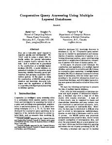
Fig. 1. Execution time and similarity. From top to bottom the graphs in each row correspond to the ontology-query pairs A-AQ4, A-AQ5, S-SQ5 and P5S-PQ5.


13

obtained. If all of them are dispatched to the database, performance may be significantly compromised. For this reason we slightly delay the addition of the new rewritings to the execution queue, by computing first all the rewritings of a stride, check for redundancies and add only the non-redundant ones to the queue. The structure of the Requiem algorithm does not allow for a directly comparable optimization strategy. Therefore, in our implementation of Requiem we add the rewritings to the queue upon their computation only during saturation (which corresponds roughly to sr-resolution). During unfolding (which corresponds roughly to sp-resolution), we compute the rewritings, checking in parallel for redundancies. The resulting rewritings are added to the queue all together, at the end of the unfolding. The redundancy check was incorporated in an optimized way, which reduced significantly the number of inferences of the original implementation. We present the results for the A and S ontologies [7], as well as for P5S, a modified version of P5, in which we have included some subconcepts for the PathX concepts of P5. We evaluate ontology A with queries AQ4, AQ5, and ontologies S and P5S with queries SQ5 and PQ5 respectively (due to restricted space we do not present the results of all ontologies and queries in [7], we choose the particular combinations as most representative of several diverse cases). We populated the ABoxes according to [9]. The results are shown in Fig. 1. In each row, the lhs graphs present the total number of retrieved answers vs time and the rhs graphs the evolution of similarity as new answers are retrieved. We use thick and light lines to present the results for ProgRes and Requiem, respectively. Execution time is total time, including both rewriting computation and answer retrieval time. The small vertical bars at the two horizontal dotted lines on the top of the lhs graphs indicate the time points a new rewriting becomes available. The upper line corresponds to ProgRes, the lower to Requiem. Table 3 presents the number of rewritings and inferences. We give the no. of rewritings dispatched to the database both with and without the redundant check optimization (within square brackets). The min column shows the no. of minimal non-redundant rewritings. The inference columns show the total no. of inferences. Within parentheses are the no. of inferences during sp-resolution (unfolding) and the no. of inferences during sr-resolution (saturation). Wtihin square brackets are the total no. of inferences without the optimization. Note that some of the inferences that ProgRes performs during sp-resolution, in Requiem are performed during saturation. Ontology A is to a large extent taxonomic. Both queries AQ4 and AQ5 produce many non-redundant rewritings, after a long sp-resolution/unfolding phase. ProgRes performs more sp-resolutions than Requiem, because the optimization introduced in the unfolding phase of Requiem removes early some redundant intermediate results and so subsequent redundant inferences are avoided. In ProgRes the respective optimization is done at the end of each stride, it is more local in nature and hence cannot always prevent a large number of redundant inferences at a global level. This is more obvious in ontology S, where ProgRes produces a lot of redundant queries. This is however an extreme degenerate case:

14


SQ5 is a bad query as half of its atoms are redundant. Back to ontology A, we note that although ProgRes needs slightly more time to compute the rewritings, it terminates faster. This is due to the progressive nature of ProgRes. While the producer thread computes the query rewritings, the consumer thread executes the already available ones, so there is no significant idle time for the consumer thread. In contrast, in Requiem most rewritings are obtained at the end of the unique unfolding phase. This demonstrates the significant benefit from progressively computing and evaluating the query rewritings. The situation is quite different in ontology P5S, in which the inference procedure consist mainly of a chain of sr-reduction/saturation steps. Here, the strategy of ProgRes is much more efficient and scalable. It avoids a very large number of inference sequences that are guaranteed to give no new queries, by applying sr-resolution only on sink atoms. As a result, it finishes almost instantly, while Requiem needs significantly more time and inferences. It is important to note, that in this case the performance of Requiem is not scalable in the size of the query. In contrast to Requiem, almost the entire execution time of ProgRes is answer retrieval time. The synthetic nature of P5S allows us to comment also on the evolution of the similarity of the answers. In (the original) ontology P5, only sr-resolution/saturation steps are involved, hence we expect ProgRes and Requiem to compute the rewritings in the same order (but not the same fast). In ontology P5S, however, for each rewriting produced at a sr-reduction step, ProgRes computes immediately all its sp-resolutions, and so the progressive decrease of similarity is achieved. Requiem computes first all the rewritings resulting from the saturation step and then all the unfoldings, hence no ranking of the answers is possible. Similar is the situation for query AQ4. In the case of AQ5, all the rewritings have the same graph structure, so the slight fluctuations in the similarity graph for Requiem are due to the non-ordered computation of the unfoldings. A steep decrease in the similarity measure occurs only when the structure of a rewriting w.r.t the original query changes. Table 3. Number of rewritings and inferences for ProgRes and Requiem. ontology/ query A AQ4 A AQ5 S SQ5 P5S PQ5

6

no. of ProgRes 320 [322] 624 [624] 128 [910] 76 [76]

rewritings no. of inferences Requiem min ProgRes Requiem 228 [256] 224 575 (507/68) [585] 453 (322/131) 624 [624] 624 1443 (1324/119) [1482] 1013 (811/202) 9 [840] 8 906 (900/6) [4422] 295 (271/24) 76 [76] 76 95 (75/20) [95] 11424 (74/11350)

[767] [1013] [2291] [11424]

Conclusions and future work

We have presented a systematic approach to the problem of stratifying over time the execution of CQA algorithms. We introduced the notions of progressive


15

CQA algorithms (sequences of CQAs - its components), of strides (result sets of subsets of the components), of ordering of strides measuring the relevance of the answers with the user query and of sorted progressive CQAs ensuring a controllable approximation of the correct answer set. We have also presented a practical algorithm for progressive CQA in DL-LiteR that implements the above ideas and showed that it is possible to develop progressive algorithms that are efficient. Actually, it has been found that in the presence of large queries and TBoxes that are not simple taxonomies of atomic concepts the proposed algorithm is much more efficient than the similar non-progressive ones (overcoming a strong limitation of some DL-LiteR CQA systems). An obvious advantage of the specific approach is the ability to be responsive even in cases of huge databases under a predetermined approximation strategy. A second advantage is that in case of inconsistency and considering data as stronger than theory (in information retrieval this is reasonable), PCQAs ensure a decreased possibility of incorrect answers. Finally, PCQA have ideal structure for parallel processing. The main disadvantage is that it is difficult to reduce the redundancies, since the complete set of answers is not available before the output. The present work can be extended in several directions. We could take advantage of the ideas presented in [10] and dramatically improved the performance of DL-LiteR CQAs. Also, we could develop PCQA algorithms and systems for more expressive DLs. Finally, we could try to stratify smaller strides in ProgRes avoiding wide replications by applying sophisticated redundancy checking.

References 1. A. Poggi, D. Lembo, D. Calvanese, G. De Giacomo, M. Lenzerini, and R. Rosati. Linking data to ontologies. J. on Data Semantics, pp. 133–173 (2008) 2. F. Baader, D. Calvanese, D. McGuinness, D. Nardi, and P. F. Patel-Schneider, editors. The Description Logic Handbook: Theory, Implementation, and Applications. Cambridge University Press (2007) 3. B. Motik et al (editors). OWL 2 web ontology language profiles. W3C Recommendation, 27 October (2009) 4. A. Artale, D. Calvanese, R. Kontchakov, and M. Zakharyaschev. The DL-Lite family and relations. Journal of Artificial Intelligence Research, pp. 36–69 (2009). 5. J. A. Robinson and A. Voronkov, editors. Handbook of Automated Reasoning (in 2 volumes). Elsevier and MIT Press (2001) 6. B. Glimm, I. Horrocks, C. Lutz, and U. Sattler. Conjunctive query answering for the description logic SHIQ. J. of Artificial Intelligence Research, 31:157–204 (2008) 7. H. Perez-Urbina, I. Horrocks, and B. Motik. Efficient query answering for OWL 2. In: 8th International Semantic Web Conference (ISWC 2009), vol. 5823 of Lecture Notes in Computer Science, pp. 489–504. Springer (2009) 8. Y. Guo, Z. Pan, and J. Heflin. An Evaluation of Knowledge Base Systems for Large OWL Datasets. Third International Semantic Web Conference, Hiroshima, Japan, LNCS 3298, Spinger (c), pp. 274-288 (2004) 9. G. Stoilos, B. Cuenca Grau, and I. Horrocks. How Incomplete is your Semantic Web Reasoner? In: 20th Nat. Conf. on Artificial Intelligence (AAAI) (2010)

16


10. Riccardo Rosati and Alessandro Almatelli, Improving Query Answering over DLLite Ontologies. In: Twelfth International Conference on Principles of Knowledge Representation and Reasoning (KR 2010) (2010) 11. H. Bunke, Graph matching: theoretical foundations, algorithms, and applications. In: Vision Interface 2000, pp. 82–88. Montreal/Canada (2000) 12. M. Dehmer, F. Emmert-Streib, A. Mehler and J. Kilian, Measuring the structural similarity of web-based documents: a novel approach, J. Comp. Intell., pp. 1-7 (2006) 13. J. Euzenat and P. Shvaiko, Ontology Matching, Springer-Verlag (2007)