Projected Wavefunctions and High Temperature Superconductivity

Projected Wavefunctions and High Temperature Superconductivity Arun Paramekanti, Mohit Randeria and Nandini Trivedi

arXiv:cond-mat/0101121v2 [cond-mat.supr-con] 30 Mar 2001

Department of Theoretical Physics, Tata Institute of Fundamental Research, Mumbai 400005, India We study the Hubbard model with parameters relevant to the cuprates, using variational Monte Carlo with projected d-wave states. For doping 0 < x < ∼ 0.35 we obtain a superconductor whose order parameter tracks the observed nonmonotonic Tc (x). The variational parameter ∆var (x) scales with the (π, 0) “hump” and T ∗ seen in photoemission. Projection leads to incoherence in the spectral function and from the singular behavior of its moments we obtain the nodal quasiparticle weight Z ∼ x though the Fermi velocity remains finite as x → 0. The Drude weight Dlow and superfluid density are consistent with experiment and Dlow ∼ Z. PACS numbers: 74.20.-z, 74.20.Fg, 74.25.-q, 74.72.-h (February 1, 2008)

Strong correlations are essential to understand d-wave high temperature superconductivity in doped Mott insulators [1]. The no-double occupancy constraint arising from strong correlations has been treated within two complementary approaches. Within the gauge theory approach [2], which is valid at all temperatures, the constraint necessitates the inclusion of strong gauge fluctuations. Alternatively, the constraint can be implemented exactly at T = 0 using the variational Monte Carlo (VMC) method. Previous variational studies [3–6] have focussed primarily on the energetics of competing states. In this letter, we revisit projected wavefunctions of the form proposed by Anderson in 1987 [1]. We compute physically interesting correlations using VMC and show that projection leads to loss of coherence. We obtain information about low energy excitations from the singular behavior of moments of the occupied spectral function. Remarkably, our results for various observables are in semi-quantitative agreement with experiments on the cuprates. We also make qualitative predictions for the doping (x) dependence of correlation functions in projected states (for x ≪ 1) from general arguments which are largely independent of the detailed form of the wavefunction and the Hamiltonian. We use the Hubbard Hamiltonian H = K + Hint . P † The kinetic energy K = k,σ ǫ(k)ckσ ckσ with ǫ(k) = −2t (cos kx + cos ky ) + 4t′ cos kx cos ky the dispersion on ′ a square lattice with nearest (t) and next-near P (t ) hopping. The on-site repulsion is Hint = U r n↑ (r)n↓ (r) with nσ (r) = c†σ (r)cσ (r). We work in the strongly correlated regime where J = 4t2 /U, t′ < ∼ t ≪ U near half filling: n = 1 − x with the hole doping x ≪ 1. We choose t′ = t/4, t = 300meV and U = 12t, so that J = 100meV consistent with neutron data on cuprates. We describe the ground state by the wavefunction |Ψ0 i = exp(iS)P|ΨBCS i.

µvar and ∆var determine ϕ(k) through ξk = ǫ(k) − µvar and Q ∆k = ∆var (cos kx − cos ky ) /2. The projector P = r (1 − n↑ (r)n↓ (r)) in Eq. (1) eliminates all configurations with double occupancy, as appropriate for U → ∞. The unitary transformation exp(iS) includes double occupancy perturbatively in t/U [7]. The transformation exp(−iS)H exp(iS) is well known to lead to the tJ Hamiltonian [7]. We emphasize that our approach effectively transforms all operators, and not only ˜ ˜ H. Using hΨ0 |Q|Ψ0 i = hΨBCS |P QP|Ψ BCS i with Q = exp(−iS)Q exp(iS), it follows that incorporating exp(iS) in the wavefunction (1) is equivalent to transforming ˜ and working with fully projected states. Q→Q Using standard VMC techniques [8] we compute equal-time correlators in the state |Ψ0 i. The two variational parameters are determined by minimizing hΨ0 |H|Ψ0 i/hΨ0 |Ψ0 i at each x. The doping dependence of the resulting ∆var (x) is shown in Fig. 1(a). Varying input parameters in H we find that the scale for ∆var is mainly determined by J = 4t2 /U . We show below that ∆var is not proportional to the SC order parameter, in contrast to BCS theory, and also argue that it is not equal to the spectral gap. On the other hand, we find that the optimal µvar (x) ≈ µ0 (x), the chemical potential of noninteracting electrons described by K. However, µvar is quite different [9] from the chemical potential µ = ∂hHi/∂N , where h· · ·i denotes the expectation value in the optimal, normalized ground state. Phase Diagram: We now show that the wavefunction (1) is able to describe three phases: a resonating valence bond (RVB) insulator, a d-wave SC and a Fermi liquid metal. To establish the T = 0 phase diagram we first study off-diagonal long range order (ODLRO) usˆ where ing Fα,β (r − r′ ) = hc†↑ (r)c†↓ (r + α ˆ )c↓ (r′ )c↑ (r′ + β)i, α ˆ , βˆ = x ˆ, yˆ. We find that Fα,β → ±Φ2 for large |r − r′ |, ˆ indicating with + (−) sign obtained for α ˆ k (⊥) to β, d-wave SC. As seen from Fig. 1(b) the order parameter Φ(x) is not proportional to ∆var (x), and is nonmonotonic. Φ vanishes linearly in x as x → 0 as first noted in ref. [4], even though ∆var 6= 0. We argue [10] that Φ ∼ x is a general property of projected SC wavefunctions. The lo-

(1)

P N/2 † † Here |ΨBCS i = ϕ(k)c c |0i is the N k k↑ −k↓ electron d-wave p BCS wave function with ϕ(k) = vk /uk = ∆k /[ξk + ξk2 + ∆2k ]. The two variational parameters 1

cal correlations can be expressed as equal-time correlators, calculable R ∞ in our formalism. Specifically, we look at Mℓ (k) = −∞ dωω ℓ f (ω)A(k, ω), where A(k, ω) is the one-particle spectral function and, at T = 0, f (ω) = Θ(−ω). We calculate M0 (k) = n(k) and the first moment [13] M1 (k) = hc†kσ [H, ckσ ]i to obtain important information about the spectral function. Nodal Quasiparticles: Fig. 2(c) shows that along (0, 0) to (π, π) n(k) has a jump discontinuity. This implies the existence of gapless quasiparticles (QPs) observed by angle resolved photoemission spectroscopy (ARPES) [14]. The spectral function along the diagonal thus has the low energy form: A(k, ω) = Zδ(ω − ξ˜k ) + Ainc , where ξ˜k = vF (k − kF ) is the QP dispersion and Ainc the smooth incoherent part. We estimate the nodal kF (x) from the location of the discontinuity and the QP weight Z from its magnitude. While kF (x) has weak doping dependence, Z(x) is shown in Fig. 2(d), with Z ∼ x as the insulator is approached [15]. Projection leads to a suppression of Z from unity with the incoherent weight (1−Z) spread out to high energies. We infer large incoherent linewidths as follows. (a) At the “band bottom” n(k = (0, 0)) ≃ 0.85 (for x = 0.18) implying that 15% of the spectral weight must have spilled over to ω > 0. (b) Even at kF , the first moment M1 lies significantly below ω = 0 (defined by the chemical potential µ = ∂hHi/∂N ); see Fig. 3(a). The moments are dominated by the high energy incoherent part of A(k, ω), but their singular behavior is determined by the gapless coherent QPs. Specifically, along the zone diagonal M1 (k) = Z ξ˜k Θ(−ξ˜k ) + smooth part. Thus its slope dM1 (k)/dk has a discontinuity of ZvF at kF , as seen in Fig. 3(a), and may be used to estimate [16] the nodal Fermi velocity vF . As seen from Fig. 3(b), vF (x) is reduced from its bare value vF0 and is weakly doping dependent, consistent with the ARPES estimate [14] of vF ≈ 1.5eV -˚ A in Bi2 Sr2 CaCu2 O8+δ (BSCCO). As x → 0, Z = [1 − ∂Σ′ /∂ω]−1 ∼ x, while vF (x)/vF0 = Z[1+(vF0 )−1 ∂Σ′ /∂k] is weakly x-dependent. This implies a 1/x divergence in the k-dependence of the self energy Σ on the zone diagonal, which could be tested by ARPES. Within slave boson mean field theory (MFT) [1], we find [9] Z sb=x in Fig.2(d) and vFsb (x) shown in Fig.3(b), both systematically smaller than the corresponding VMC results. Thus the holons and spinons must be partially bound by gauge fluctuations beyond MFT. Moments Along (π, 0) → (π, π): The moments n(k) and M1 (k) near k = (π, 0) are not sufficient to estimate the SC gap, however they give insight into the nature of the spectral function. As seen from Fig. 4(a) n(k) is much broader than that for the unprojected |ΨBCS i. For k’s near (π, π), which correspond to high energy, unoccupied (ω > 0) states in |ΨBCS i we see a significant build up of spectral weight transferred from ω < 0. Correspondingly, we see loss of spectral weight near (π, 0). We thus infer large linewidths at all k’s, also seen from the large |M1 (k)| (in Fig. 4(b)) relative to the BCS result.

cal fixed number constraint imposed by P at x = 0 leads to large quantum phase fluctuations that destroy SC order. The non-SC state at x = 0 is an insulator with a vanishing Drude weight, as shown below. The system is a SC in the doping range 0 < x < xc ≃ 0.35 with Φ 6= 0. For x > xc , Φ = 0 and the wavefunction Ψ0 for ∆var = 0 describes a normal Fermi liquid. In the remainder of this paper we will study 0 ≤ x ≤ xc .

FIG. 1. (a): The variational parameter ∆var (filled squares) and the (π, 0) hump scale (open triangles) in ARPES [11] versus doping. (b): Doping dependence of the d-wave SC order parameter Φ. Solid lines in (a) and (b) are guides to √ the eye. (c): The coherence length ξsc ≥ max(ξpair , 1/ x).

Coherence Lengths: We must carefully distinguish between various ‘coherence lengths’, which are the same in BCS theory, but are very different in strongly correlated SC’s. The internal pair wavefunction ϕ(k) defines a pair-size ξpair ∼ v¯F0 /∆var , where v¯F0 is the bare average Fermi velocity. Projection does not affect the pair-size much, and ξpair remains finite at x = 0, where it defines the range of singlet bonds in the RVB insulator [1]. A second important length scale is the inter-hole spac√ ing 1/ x. At shorter distances there are no holes and the system effectively looks like the x = 0 insulator. Thus the superconducting coherence√length ξsc must necessarily satisfy ξsc ≥ max (ξpair , 1/ x). This bound implies that ξsc must diverge both in the insulating limit x → 0 (see also Refs. [2]) and the metallic limit x → x− c , but is small at optimality; see Fig. 1(c). This non-monotonic behavior of ξsc (x) should be checked experimentally. Momentum Distribution: From gray-scale plots like Fig. 2 we see considerable structure in the momentum distribution n(k) over the entire range 0 ≤ x ≤ xc . One cannot define a Fermi surface (FS) since the system is a SC (or an insulator). Nevertheless, for all x, the k-space loci (i) on which n(k) = 1/2 and (ii) on which |∇k n(k)| is maximum, are both quite similar to the corresponding noninteracting FS’s. For t′ = t/4, the FS is hole-like for x< ∼ 0.22, and electron-like for overdoping [12]. We next exploit the fact that moments of dynami2

The transfer of weight over large energies inferred above suggests that projection pushes spectral weight to |ω| < ∆var , the gap in unprojected BCS theory. We thus expect that the true spectral gap Egap < ∆var and that the coherent QP near (π, 0) must then reside at Egap in order to be stable against decay into incoherent excitations. It is then plausible that ∆var , the large gap before projection, is related to an incoherent feature in A(k, ω) near (π, 0) after projection [17]. Indeed, comparing ∆var with the (π, 0) “hump” feature seen in ARPES [11], we find good agreement in the magnitude as well as doping dependence; see Fig. 1(a). Optical spectral Rweight: The optical P conductivity ∞ sum rule states that 0 dωReσ(ω) = π k m−1
(k)n(k) ≡ πDtot /2 where m−1 (k) = ∂ 2 ǫ(k)/∂kx ∂kx is the noninteracting mass tensor (we set ¯h = c = e = 1). The total optical spectral weight Dtot (x) is plotted in Fig. 5(a) and seen to be non-zero even at x = 0, since the infinite cutoff in the integral above includes contributions from the “upper Hubbard band”. A physically more interesting quantity is the low frequency optical weight, or Drude weight, Dlow where the upper cutoff extends above the scale of t and J, but is much smaller than U . This is conveniently defined [9] by the response to an external vector potential: Dlow = ∂ 2 hHA iA /∂A2 . Here the subscript on H denotes that A enters the kinetic energy via a Peierls minimal coupling, and that on the expectation value denotes the corresponding modification of exp(iS) in Eq. (1). The Drude weight Dlow (x), plotted in Fig. 5(a), vanishes linearly as x → 0, which can be argued to be a general property of projected states [9]. This also proves, following Ref. [18], that |Ψ0 i describes an insulator at x = 0. Both the magnitude and doping dependence of Dlow (x) are consistent with optical data on the cuprates [19]. Motivated by our results on the nodal Z(x) and Dlow (x), we make a parametric plot of these two quantities in Fig. 5(b) and find that Dlow ∼ Z over the entire doping range, a prediction which can be checked by comparing optics and ARPES [20] on the cuprates. Superfluid Density: The Kubo formula for the superfluid stiffness Ds can be written as Ds = Dlow − ΛT , where Dlow is the diamagnetic response, and ΛT is the transverse current-current correlator. Using the spectral representation for ΛT it is easy to see that [21] ΛT ≥ 0 implying Ds ≤ Dlow . Two conclusions follow. First, Ds → 0 as x → 0, consistent with experiments [22]. Second, we obtain a lower bound on the penetration depth 2 λL defined by λ−2 h2 c2 dc . Using the calcuL ≡ 4πe Ds /¯ lated Dlow ≈ 90meV at optimality and a mean interlayer spacing dc = 7.5˚ A (appropriate to BSCCO), we find λL > A, consistent with experiment [23]. ∼ 1350˚ Conclusions: We have shown, within our variational scheme, the T = 0 evolution of the system from an undoped insulator to a d-wave SC to a Fermi liquid as a function of x. The SC order parameter Φ(x) is nonmonotonic with a maximum at optimal doping x ≃ 0.2,

kF

(a)

(c)

n(k) Z x=0.18 x=0.05

(π,π)

k

(d)

α

(b)

(0,0)

Z

β Z

x=0.18

sb

Doping (x)

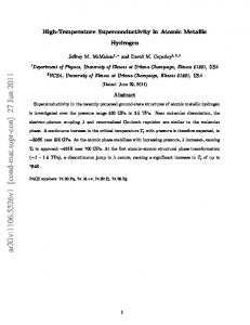
FIG. 2. (a) and (b): Gray-scale plots of n(k) (black ≡ 1, white ≡ 0) centered at k = (0, 0) for x = 0.05 and x = 0.18 respectively on a 19 × 19 + 1 lattice, showing very little doping dependence of the large “Fermi surface”. (c): n(k) plotted along the diagonal direction (indicated as α in Panel (b)), showing the jump at kF which implies a gapless nodal quasiparticle of weight Z. (d): Nodal quasiparticle weight Z(x), compared with the slave boson mean field Z sb (x) (dashed line).

k

F

x=0.18 (0,0)

(π,π)

FIG. 3. (a): The moment M1 (k) along the zone diagonal, with smooth fits for k < kF and k > kF , showing a discontinuity of ZvF in its slope at kF . (b): Doping dependence of the nodal quasiparticle velocity obtained from M1 (k). Error bars come from fits to M1 (k) and errors in Z. Also shown are the bare nodal velocity vF0 , the slave boson mean field vFsb (x) (expt) (dashed line), and the ARPES estimate vF [14].

suggestive of the experimental trend in Tc (x) from underto over-doping. As x → 0 Ds vanishes, while the spectral gap, expected to scale with ∆var , remains finite. Thus the underdoped state, with strong pairing and weak phase coherence, should lead to pseudogap behavior in the temperature range between Tc (which scales like Φ) and T ∗ (which scales like ∆var ). 3

[3] C. Gros, R. Joynt and T.M. Rice, Z. Phys. B 68, 425 (1987); E.S. Heeb and T.M. Rice, Europhys. Lett. 27, 673 (1994). [4] C. Gros, Phys. Rev. B 38, 931 (1988). [5] H. Yokoyama and H. Shiba, J. Phys. Soc. Jpn. 57, 2482 (1988); H. Yokoyama and M. Ogata, J. Phys. Soc. Jpn. 65, 3615 (1996). [6] F. Becca, M. Capone, and S. Sorella, Phys. Rev. B 62, 12700 (2000). [7] C. Gros, R. Joynt and T.M. Rice, Phys. Rev. B 36, 381 (1987); A.H. Macdonald, S.M. Girvin and D. Yoshioka, Phys. Rev. B 37, 9753 (1988). [8] Since the pair wavefunction ϕ(k) is singular on the zone diagonal we use “tilted” lattices [3] with periodic boundary conditions. Most results were obtained on a 15×15+1 site lattice, with some on a 19×19+1 lattice. Typically we used 5000 equilibriation sweeps, and averaged over 5001000 configurations from 5000 sweeps. In all the VMC results presented here, the error bars are of the size of the symbol, unless explicitly shown. [9] Details will be presented in a longer paper; A. Paramekanti, M. Randeria and N. Trivedi (unpublished). [10] To put a pair of electrons on a link near r, after removing them from a link near the origin, requires two vacancies near r. Thus Fα,α (r) ∼ x2 and Φ ∼ x as x → 0. [11] J-C. Campuzano et al., Phys. Rev. Lett. 83, 3709 (1999). [12] A. Ino et al., cond-mat/0005370. [13] The Fourier transform of M1 (k) is M1 (r − r′ ) = −trr′ hc†σ (r)cσ (r′ )i + U hc†σ (r)cσ (r′ )nσ (r′ )i. Since the second term is O(U ) we need S in Eq. (1) to O(t/U )2 to obtain M1 (k) correctly to O(J). [14] A. Kaminski et al., Phys. Rev. Lett. 84, 1788 (2000); and Phys. Rev. Lett. 86, 1070 (2001). [15] Relating Z to the amplitude of the asymptotic powerlaw decay in hc†σ (r)cσ (r′ )i we can show that Z ∼ x for projected states [9]. [16] For unprojected BCS wavefunctions we can estimate vF with 5% accuracy using this method on finite systems. [17] Numerically |M1 (π, 0) − M1 (kFnode )| ∼ ∆var for all x. [18] A.J. Millis and S.N. Coppersmith, Phys. Rev. B 42, 10807 (1990) and Phys. Rev. B 43, 13770 (1991). [19] Using a lattice spacing a = 3.85˚ A for BSCCO we find (ωp∗ )2 ≡ (4πe2 /a)Dlow ≈ (1.8eV )2 at optimal doping, in good agreement with data summarized in S.L. Cooper et al., Phys. Rev. B 47, 8233 (1993). [20] D.L. Feng et al, Science 280, 277 (2000) and H. Ding et al, cond-mat/0006143, find that the anti-nodal quasiparticle weight scales with the superfluid density. [21] A. Paramekanti, N. Trivedi and M. Randeria, Phys. Rev. B 57, 11639 (1998). [22] Y.J. Uemura et al., Phys. Rev. Lett. 62, 2317 (1989). [23] The agreement with the measured λ ≃ 2100˚ A in optimal BSCCO [S.F. Lee et al., Phys. Rev. Lett. 77, 735 (1996)] would be improved by including the effects of long wavelength quantum phase fluctuations; see A. Paramekanti et al, Phys. Rev. B 62, 6786 (2000), L. Benfatto et al, cond-mat/0008100.

FIG. 4. (a): n(k) plotted along the (π, 0)-(π, π) direction (indicated as β in Fig. 2(b)) and compared with the BCS result. (b): The moment M1 (k) plotted along the (π, 0)-(π, π) direction compared with the BCS values.

FIG. 5. (a): Doping dependence of the total (Dtot ) and low energy (Dlow ) optical spectral weights (b): The optical spectral weight Dlow versus the nodal quasiparticle weight Z.

Acknowledgements: We thank H.R. Krishnamurthy, P.A. Lee, M.R. Norman and J. Orenstein for helpful comments on an earlier draft. M.R. was supported in part by the DST through the Swarnajayanti scheme.

[1] P.W. Anderson, Science 235, 1196 (1987); G. Baskaran, Z. Zou and P.W. Anderson, Sol. St. Comm. 63, 973 (1987); G. Kotliar and J. Liu, Phys. Rev. B 38, 5142 (1988). [2] X. G. Wen and P. A. Lee, Phys. Rev. Lett. 78, 4111 (1997); D. H. Lee, Phys. Rev. Lett. 84, 2694 (2000).

4