suitable θ reflects the problem-solving nature of SLD-resolution. When the unifi- cation algorithm underlying SLD-resol
Proof Relevant Corecursive Resolution Peng Fu1? , Ekaterina Komendantskaya1 , Tom Schrijvers2 , Andrew Pond1?? 1
2
Computer Science, University of Dundee Department of Computer Science, KU Leuven
Abstract. Resolution lies at the foundation of both logic programming and type class context reduction in functional languages. Terminating derivations by resolution have well-defined inductive meaning, whereas some non-terminating derivations can be understood coinductively. Cycle detection is a popular method to capture a small subset of such derivations. We show that in fact cycle detection is a restricted form of coinductive proof, in which the atomic formula forming the cycle plays the rˆ ole of coinductive hypothesis. This paper introduces a heuristic method for obtaining richer coinductive hypotheses in the form of Horn formulas. Our approach subsumes cycle detection and gives coinductive meaning to a larger class of derivations. For this purpose we extend resolution with Horn formula resolvents and corecursive evidence generation. We illustrate our method on nonterminating type class resolution problems. Keywords: Horn Clause Logic, Resolution, Corecursion, Haskell Type Class Inference, Coinductive Proofs.
1
Introduction
Horn clause logic is a fragment of first-order logic known for its simple syntax, well-defined models, and efficient algorithms for automated proof search. It is used in a variety of applications, from program verification [3] to type inference in object-oriented programming languages [1]. Similar syntax and proof methods underlie type class inference in functional programming languages [24,17]. For example, the following declaration specifies equality class instances for pairs and integers in Haskell: instance Eq Int where ... instance (Eq x , Eq y) ⇒ Eq (x , y) where ... It corresponds to a Horn clause program ΦPair with two clauses κInt and κPair : κInt : Eq Int κPair : (Eq x , Eq y) ⇒ Eq (x , y) Horn clause logic uses SLD-resolution as an inference engine. If a derivation for a given formula A and a Horn clause program Φ terminates successfully with ? ??
This author is supported by EPSRC grant EP/K031864/1. This author is supported by Carnegie Trust Scotland.
substitution θ, then θA is logically entailed by Φ, or Φ ` θA. The search for a suitable θ reflects the problem-solving nature of SLD-resolution. When the unification algorithm underlying SLD-resolution is restricted to matching, resolution can be viewed as theorem proving: the successful terminating derivations for A using Φ will guarantee Φ ` A. For example, Eq (Int, Int) Eq Int, Eq Int Eq Int ∅. Therefore, we have: ΦPair ` Eq (Int, Int). For the purposes of this paper, we always assume resolution by term-matching. To emphasize the proof-theoretic meaning of resolution, we will record proof evidence alongside the derivation steps. For instance, Eq (Int, Int) is proven by applying the clauses κPair and κInt . We denote this by ΦPair ` Eq (Int, Int) ⇓ κPair κInt κInt . Horn clause logic can have inductive and coinductive interpretation, via the least and greatest fixed points of the consequence operator FΦ . Given a Horn clause program Φ, and a set S containing (ground) formulas formed from the signature of Φ, FΦ (S) = {σA | σB1 , . . . , σBn ∈ S and B1 , . . . Bn ⇒ A ∈ Φ} [18]. Through the Knaster-Tarski construction, the least fixed point of this operator gives the set of all finite ground formulas inductively entailed by Φ. Extending S to include infinite terms, the greatest fixed point of FΦ defines the set of all finite and infinite ground formulas coinductively entailed by Φ. Inductively, SLD-resolution is sound: if Φ ` A, then A is inductively entailed by Φ. It is more difficult to characterise coinductive entailment computationally; several approaches exist [22,18,16]. So far the most popular solution is to use cycle detection [22]: given a Horn clause program Φ, if a cycle is found in a derivation for a formula A, then A is coinductively entailed by Φ. Consider, as an example, the following Horn clause program ΦAB : κA : B x ⇒ A x κB : A x ⇒ B x It gives rise to an infinite derivation A x B x A x . . .. By noticing the cycle, we can conclude that (an instance) of A x is coinductively entailed by ΦAB . We can construct a proof evidence that reflects the circular nature of this derivation: α = κA (κB α). This being a recursive equation expecting the greatest fixed point solution, we can represent it with the greatest fix point ν operator, να.κA (κB α). Now we have ΦAB ` A x ⇓ να.κA (κB α). From now on, we call the evidence containing ν-term a corecursive evidence. According to Gibbons and Hutton [7] and inspired by Moss and Danner [20], a corecursive program is defined to be a function whose range is a type defined recursively as the greatest solution of some equation (i.e. whose range is a coinductive type). We can informally understand the Horn clause ΦAB as the following Haskell data type declarations: data B x = KB (A x ) data A x = KA (B x ) So the corecursive evidence να.κA (κB α) for A x corresponds to the corecursive program (d :: A x) = KA (KB d). In our case, the corecursive evidence d is that function, and its range type A x can be seen as a coinductive type. 2
Corecursion also arises in type class inference. Consider the following mutually recursive definitions of lists of even and odd length in Haskell: data OddList a = OCons a (EvenList a) data EvenList a = Nil | ECons a (OddList a) They give rise to Eq type class instance declarations that can be expressed using the following Horn clause program ΦEvenOdd : κOdd : (Eq a, Eq (EvenList a)) ⇒ Eq (OddList a) κEven : (Eq a, Eq (OddList a)) ⇒ Eq (EvenList a) When resolving the type class constraint Eq (OddList Int), Haskell’s standard type class resolution diverges. The state-of-the-art is to use cycle detection [17] to terminate otherwise infinite derivations. Resolution for Eq (OddList Int) exhibits a cycle on the atomic formula Eq (OddList Int), thus the derivation can be terminated, with corecursive evidence να.κOdd κInt (κEven κInt α). The method of cycle detection is rather limited: there are many Horn clause programs that have coinductive meaning, but do not give rise to detectable cycles. For example, consider the program ΦQ : κS : (Q (S (G x )), Q x ) ⇒ Q (S x ) κG : Q x ⇒ Q (G x ) κZ : Q Z It gives rise to the following derivation without cycling: Q Z, Q (S (G Z)) Q Z, Q (G Z), Q (S (G (G Z))) . . .. When Q (S Z) such derivations arise, we cannot terminate the derivation by cycle detection. Let us look at a similar situation for type classes. Consider a datatype-generic representation of perfect trees: a nested datatype [2], with fixpoint Mu of the higher-order functor HPTree [12]. data Mu h a = In {out :: h (Mu h) a } data HPTree f a = HPLeaf a | HPNode (f (a, a)) These two datatypes give rise to the following Eq type class instances. instance Eq (h (Mu h) a) ⇒ Eq (Mu h a) where In x ≡ In y = x ≡ y instance (Eq a, Eq (f (a, a))) ⇒ Eq (HPTree f a) where HPLeaf x ≡ HPLeaf y = x ≡ y HPNode xs ≡ HPNode ys = xs ≡ ys ≡ = False The corresponding Horn clause program ΦHP T ree consists of ΦP air and the following two clauses : κMu : Eq (h (Mu h) a) ⇒ Eq (Mu h a) κHPTree : (Eq a, Eq (f (a, a))) ⇒ Eq (HPTree f a) 3
The type class resolution for Eq (Mu HPTree Int) cannot be terminated by cycle detection. Instead we get a context reduction overflow error in the Glasgow Haskell Compiler, even if we just compare two finite data structures of the type Mu HPTree Int. To find a solution to the above problems, let us view infinite resolution from the perspective of coinductive proof in the Calculus of Coinductive Constructions [4,8]. There, in order to prove a proposition F from the assumptions F1 , .., Fn , the proof may involve not only natural deduction and lemmas, but also F , provided the use of F is guarded. We could say that the existing cycle detection methods treat the atomic formula forming a cycle as a coinductive hypothesis. We can equivalently describe the above-explained derivation for ΦAB in the following terms: when a cycle with a formula A x is found in the derivation, ΦAB gets extended with a coinductive hypothesis α : A x . So to prove A x coinductively, we would need to apply the clause κA first, and then clause κB , finally apply the coinductive hypothesis. The resulting proof witness is να. κA (κB α). The next logical step we can make is to use the above formalism to extend the syntax of the coinductive hypotheses. While cycle detection only uses atomic formulas as coinductive hypotheses, we can try to generalise the syntax of coinductive hypotheses to full Horn formulas. For example, for program ΦQ , we could prove a lemma e : Q x ⇒ Q (S x ) coinductively, which would allow us to form finite derivation for Q (S Z ), which is described by (e κZ ). The proof of e : Q x ⇒ Q (S x ) is of a coinductive nature: if we first assume α : Q x ⇒ Q (S x ) and α1 : Q C, then all we need to show is Q (S C ).3 To show Q (S C ), we apply κS , which gives us Q C , Q (S (G C )). We first discharge Q C with α1 and then apply the coinductive hypothesis α which yields Q (G C ), and can be proved with κG and α1 . So we have obtained a coinductive proof for e, which is να.λα1 .κS (α (κG α1 )) α1 . We can apply similar reasoning to show that ΦHPTree ` Eq (Mu HPTree Int) ⇓ (να.λα1 .κMu (κHPTree α1 (α (κPair α1 α1 )))) κInt using the coinductively proved lemma Eq x ⇒ Eq (Mu HPTree x ) 4 . To formalise the above intuitions, we need to solve several technical problems. 1. How to generate suitable lemmas? We propose to observe a more general notion of a loop invariant than a cycle in the non-terminating resolution. In Section 3 we devise a heuristic method to identify potential loops in the resolution tree and extract candidate lemmas in Horn clause form. In general, it is very challenging to develop a practical method for generating candidate lemmas based on loop analysis, since the admissibility of a loop in reduction is a semi-decidable problem [25]. 2. How to enrich resolution to allow coinductive proofs for Horn formulas? and how to formalise the corecursive proof evidence construction? Coinductive proofs involve not only applying the axioms, but also modus ponens and generalization. Therefore, the resolution mechanism will have to be extended in order to support such automation. 3 4
Note that here C is an eigenvariable. The proof term can be type-checked with polymorphic recursion.
4
In Section 4, we introduce proof relevant corecursive resolution – a calculus that extends the standard resolution rule with two further rules: one allows us to resolve Horn formula queries, and the other to construct corecursive proof evidence for non-terminating resolution. 3. How to give an operational semantics to the evidence produced by corecursive resolution of Section 4? In particular, we need to show the correspondence between corecursive evidence and resolution seen as infinite reduction. In Section 5, we prove that for every non-terminating resolution resulting from a simple loop, a coinductively provable candidate lemma can be obtained and its evidence is observationally equivalent to the non-terminating resolution process. In type class inference, the proof evidence has computational meaning, i.e. the evidence will be run as a program. So the corecursive evidence should be able to recover the original infinite resolution trace. In Sections 6 and 7 we survey the related work, explain the limitations of our method and conclude the paper. We have implemented our method of candidate lemma generation based on loop analysis and corecursive resolution, and incorporated it in the type class inference process of a simple functional language. Additional examples and implementation information are provided in the extended version.
2
Preliminaries: Resolution with Evidence
This section provides a standard formalisation of resolution with evidence together with two derived forms: a small-step variant of resolution and a reification of resolution in a resolution tree. We consider the following syntax. Definition 1 (Basic syntax). Term Atomic Formula Horn Formula Proof/Evidence Axiom Environment
t A, B, C, D H e Φ
::= ::= ::= ::= ::=
x | K | t t0 P t1 ... tn B1 , ..., Bn ⇒ A κ | e e0 · | Φ, (κ : H)
We consider first-order applicative terms, where K stands for some constant symbol. Atomic formulas are predicates on terms, and Horn formulas are defined as usual. We assume that all variables x in Horn formulas are implicitly universally quantified. There are no existential variables in the Horn formulas, S i.e., i FV(Bi ) ⊆ FV(A) for B1 , . . . , Bn ⇒ A. The axiom environment Φ is a set of Horn formulas labelled with distinct evidence constants κ. Evidence terms e are made of evidence constants κ and their applications. Finally, we often use A to abbreviate A1 , ..., An when the number n is unimportant. The above syntax can be used to model the Haskell type class setting as follows. Terms denote Haskell types like Int or (x , y), and atomic formulas denote Haskell type class constraints on types like Eq (Int, Int). Horn formulas correspond to the type-level information of type class instances. 5
Our evidence e models type class dictionaries, following Wadler and Blott’s dictionary-passing elaboration of type classes [24]. In particular the constants κ refer to dictionaries that capture the term-level information of type class instances, i.e., the implementations of the type class methods. Evidence application (e e0 ) accounts for dictionaries that are parametrised by other dictionaries. Horn formulas in turn represent type class instance declarations. The axiom environment Φ corresponds to Haskell’s global environment of type class instances. Note that the treatment of type class instance declaration and their corresponding evidence construction here are based on our own understanding of many related works ([15,14,23]), which are also discussed in Section 6. In order to define resolution together with evidence generation, we use resolution judgement Φ ` A ⇓ e to state that the atomic formula A is entailed by the axioms Φ, and that the proof term e witnesses this entailment. It is defined by means of the following inference rule. Definition 2 (Resolution). Φ ` A ⇓ e Φ ` σB1 ⇓ e1 · · · Φ ` σBn ⇓ en if (κ : B1 , ..., Bn ⇒ A) ∈ Φ Φ ` σA ⇓ κ e1 · · · en
Using this definition we can show ΦPair ` Eq (Int, Int) ⇓ κPair κInt κInt . In case resolution is diverging, it is often more convenient to consider a smallstep resolution judgement (in analogy to the small step operational semantics) that performs one resolution step at a time and allows us to observe the intermediate states. The basic idea is to rewrite the initial query A step by step into its evidence e. This involves mixed terms on the way that consist partly of evidence, and partly of formulas that are not yet resolved. Definition 3 (Mixed Terms). Mixed term Mixed term context
q C
::= ::=
A | κ | q q0 •|C q |q C
At the same time we have defined mixed term contexts C as mixed terms with a hole •, where C[q] substitutes the hole with q in the usual way. Definition 4 (Small-Step Resolution). Φ ` q → q 0 Φ ` C[σA] → C[κ σB]
if (κ : B ⇒ A) ∈ Φ
For instance, we resolve Eq (Int, Int) in three small steps: ΦPair ` Eq (Int, Int) → κPair (Eq Int) (Eq Int), ΦPair ` κPair (Eq Int) (Eq Int) → κPair κInt (Eq Int) and ΦPair ` κPair κInt (Eq Int) → κPair κInt κInt . We write Φ ` q →∗ q 0 to denote the transitive closure of small-step resolution. The following theorem formalizes the intuition that resolution and small-step resolution coincide. Theorem 1. Φ ` A ⇓ e iff Φ ` A →∗ e. 6
Eq (Mu HPTree Int) κ1Mu Eq (HPTree (Mu HPTree) Int) κ2HPTree κ1HPTree Eq Int
Eq (Mu HPTree (Int, Int)) κ1Mu
κInt �
Eq (HPTree (Mu HPTree) (Int, Int)) κ1HPTree ...
κ2HPTree ...
Fig. 1: The infinite resolution tree for ΦHPTree ` Eq (Mu HPTree Int) ⇑
The proof tree for a judgement Φ ` A ⇓ e is called a resolution tree. It conveniently records the history of resolution and, for instance, it is easy to observe the ancestors of a node. This last feature is useful for our heuristic loop invariant analysis in Section 3. Our formalisation of trees in general is as follows: We use w, v to denote positions hk1 , k2 , ..., kn i in a tree, where ki > 1 for 1 6 i 6 n. Let � denote the empty position or root. We also define hk1 , k2 , ..., kn i · i = hk1 , k2 , ..., kn , ii and hk1 , k2 , ..., kn i + hl1 , ..., lm i = hk1 , k2 , ..., kn , l1 , ..., lm i. We write w > v if there exists a non-empty v 0 such that w = v + v 0 . For a tree T , T (w) refers to the node at position w, and T (w, i) refers to the edge between T (w) and T (w · i). We use � as a special proposition to denote success. Resolution trees are defined as follows, note that they are a special case of rewriting trees [13,16]: Definition 5 (Resolution Tree). The resolution tree for atomic formula A is a tree T satisfying: – T (�) = A. – T (w · i) = σBi and T (w, i) = κi with i ∈ {1, ..., n} if T (w) = σD and (κ : B1 , ..., Bn ⇒ D) ∈ Φ. When n = 0, we write T (w·i) = � and T (w, i) = κ for any i > 0. In general, the resolution tree can be infinite, this means that resolution is non-terminating, which we denote as Φ ` A ⇑. Figure 1 shows a finite fragment of the infinite resolution tree for ΦHPTree ` Eq (Mu HPTree Int) ⇑. We note that Definitions 2 and 4 describe a special case of SLD-resolution in which unification taking place in derivations is restricted to term-matching. This restriction is motivated by two considerations. The first one comes directly from the application area of our results: type class resolution uses exactly this restricted version of SLD-resolution. The second reason is of more general nature. As discussed in detail in [6,16], SLD-derivations restricted to term-matching 7
reflect the theorem proving content of a proof by SLD-resolution. That is, if A can be derived from Φ by SLD-resolution with term-matching only, then A is inductvely entailed by Φ. If, on the other hand, A is derived from Φ by SLDresolution with unification and computes a substitution σ, then σA is inductively entailed by Φ. In this sense, SLD-resolution with unification additionally has a problem-solving aspect. In developing proof-theoretic approach to resolution here, we thus focus on resolution by term-matching. The resolution rule of Definition 2 resembles the definition of the consequence operator [18] used to define declarative semantics of Horn clause Logic. In fact, the forward and backward closure of the rule of Definition 2 can be directly used to construct the usual least and greatest Herbrand models for Horn clause logic, as shown in [16]. There, it was also shown that SLD-resolution by term-matching is sound but incomplete relative to the least Herbrand models.
3
Candidate Lemma Generation
This section explains how we generate candidate lemma from a potentially infinite resolution tree. Based on Paterson’s condition we obtain a finite pruned approximation (Definition 8) of this resolution tree. Anti-unification on this approximation yields an abstract atomic formula and the corresponding abstract approximated resolution tree. It is from this abstract tree that we read off the candidate lemma (Definition 11). We use Σ(A) and FVar(A) to denote the multi-sets of respectively function symbols and variables in A. Definition 6 (Paterson’s Condition). For (κ : B ⇒ A) ∈ Φ, we say κ satisfies Paterson’s condition if (Σ(Bi ) ∪ FVar(Bi )) ⊂ (Σ(A) ∪ FVar(A)) for each Bi . Paterson’s condition is used in Glasgow Haskell Compiler to enforce termination of context reduction [23]. In this paper, we use it as a practical criterion to detect problematic instance declarations. Any declarations that do not satisfy the condition could potentially introduce diverging behavior in the resolution tree. If κ : A1 , ..., An ⇒ B, then we have κi : Ai ⇒ B for projection on index i. Definition 7 (Critical Triple). Let v = (w · i) + v 0 for some v 0 . A critical triple in T is a triple hκi , T (w), T (v)i such that T (v, i) = T (w, i) = κi , and κi does not satisfy Paterson’s condition. We will omit κi from the triple and write hT (w), T (v)i when it is not important. Intuitively, it means the nodes T (w) and T (v) are using the same problematic projection κi , which could give rise to infinite resolution. The absence of a critical triple in a resolution tree means that it has to be finite [23], while the presence of a critical triple only means that the tree is possibly infinite. In general the infiniteness of a resolution tree is undecidable and the critical triples provide a convenient over-approximation. 8
Definition 8 (Closed Subtree). A closed subtree T is a subtree of a resolution tree such that for all leaves T (v) 6= �, the root T (�) and T (v) form a critical triple. The critical triple in Figure 1 is formed by the underlined nodes. The closed subtree in that figure is the subtree without the infinite branch below node Eq (Mu HPTree (Int, Int)). A closed subtree can intuitively be understood as a finite approximation of an infinite resolution tree. We use it as the basis for generating candidate lemma by means of anti-unification [21]. Definition 9 (Anti-Unifier). We define the least general anti-unifier of atomic formulas A and B (denoted by A t B) and the least general anti-unifier of the terms t and t0 (denoted by t t t0 ) as: – P t1 ..., tn t P t01 ..., t0n = P (t1 t t01 ) ... (tn t t0n ) – K t1 ... tn t K t01 ... t0n = K (t1 t t01 ) ... (tn t t0n ) – Otherwise, A t B = φ(A, B), t t t0 = φ(t, t0 ), where φ is an injective function from a pair of terms (atomic formulas) to a set of fresh variables. Anti-unification allows us to extract the common pattern from different ground atomic formulas. Definition 10 (Abstract Representation). Let hT (�), T (v1 )i, ..., hT (�), T (vn )i be all the critical triples in a closed subtree T . Let C = T (�) t T (v1 ) t ... t T (vn ), then the abstract representation T 0 of the closed subtree T is a tree such that: – T 0 (�) = C – T 0 (w · i) = σBi and T 0 (w, i) = κi with i ∈ {1, ..., n} if T 0 (w) = σD and (κ : B1 , ..., Bn ⇒ D) ∈ Φ. When n = 0, we write T 0 (w · i) = � and T 0 (w, i) = κ for any i > 0. – T 0 (w) is undefined if w > vi for some 1 6 i 6 n. The abstract representation unfolds the anti-unifier of all the critical triples. Thus the abstract representation can always be embedded into the original closed subtree. It is an abstract form of the closed subtree, and we can extract the candidate lemma from the abstract representation. Definition 11 (Candidate Lemma). Let T be an abstract representation of a closed subtree, then the candidate lemma induced by this abstract representation is T (v1 ), ..., T (vn ) ⇒ T (�), where the T (vi ) are all the leaves for which T (vi ) ⇒ T (�) satisfies Paterson’s condition. Figure 2 shows the abstract representation of the closed subtree of Figure 1. We read off the candidate lemma as Eq x ⇒ Eq (Mu HPTree x ). The candidate lemma plays a double role. Firstly, it allows us to construct a finite resolution tree. For example, we know that Eq (Mu HPTree Int) gives rise to infinite tree with the axiom environment ΦHPTree . However, a finite tree can be constructed with Eq x ⇒ Eq (Mu HPTree x ), since it reduces 9
Eq (Mu HPTree x ) κ1Mu Eq (HPTree (Mu HPTree) x ) κ2HPTree κ1HPTree Eq (Mu HPTree (x , x ))
Eq x
Fig. 2: The abstract representation of the closed subtree of Figure 1
Eq (Mu HPTree Int) to Eq Int, which succeeds trivially with κInt . Next we show how to prove the candidate lemma coinductively, and such proofs will encapsulate the infinite aspect of the resolution tree. Since an infinite resolution tree gives rise to infinite evidence, the finite proof of the lemma has to be coinductive. We discuss such evidence construction in detail in Section 4 and Section 5.
4
Corecursive Resolution
In this section, we extend the definition of resolution from Section 2 by introducing two additional rules: one to handle coinductive proofs, and another – to allow Horn formula goals, rather than atomic goals, in the derivations. We call the resulting calculus corecursive resolution. Definition 12 (Extended Syntax). Proof/Evidence Axiom Environment
e Φ
::= ::=
κ | e e0 | α | λα.e | να.e · | Φ, (e : H)
To support coinductive proofs, we extend the syntax of evidence with functions λα.e, variables α and fixed point να.e (which models the recursive equation α = e expecting the greatest solution). Also we allow the Horn clauses H in the axiom environment Φ to be supported by any form of evidence e (and not necessarily by constants κ). Definition 13 (Corecursive Resolution). The following judgement for corecursive resolution extends the resolution in Definition 2. Φ ` σB1 ⇓ e1 · · · Φ ` σBn ⇓ en if (e : B1 , ..., Bm ⇒ A) ∈ Φ Φ ` σA ⇓ e e1 · · · en Φ, (α : A ⇒ B) ` A ⇒ B ⇓ e Φ ` A ⇒ B ⇓ να.e
HNF(e)
(Mu)
Φ, (α : A) ` B ⇓ e (Lam) Φ ` A ⇒ B ⇓ λα.e
Note that HNF(e) means e has to be in head normal form λα.κ e. This requirement is essential to ensure the corecursive evidence satisfies the guardedness 10
condition.5 The Lam rule implicitly assumes the treatment of eigenvariables, i.e. we instantiate all the free variables in A ⇒ B with fresh term constants. We implicitly assume that axiom environments are well-formed. Definition 14 (Well-formedness of environment). · ` wf
Φ ` wf Φ, α : H ` wf
Φ ` wf Φ, κ : H ` wf
Φ`H⇓e Φ, e : H ` wf
As an example, let us consider resolving the candidate lemma Eq x ⇒ Eq (My HPTree x ) against the axiom environment ΦHPTree . This yields the following derivation, where Φ1 = ΦHPTree , (α : Eq x ⇒ Eq (Mu HPTree x )) and Φ2 = Φ1 , (α1 : Eq C ): Φ2 ` Eq C ⇓ α1 Φ2 ` Eq C ⇓ α1 Φ2 ` Eq (C , C ) ⇓ (κPair α1 α1 ) Φ2 ` Eq C ⇓ α1 Φ2 ` Eq (HPTree (C , C )) ⇓ α (κPair α1 α1 ) Φ2 ` Eq (HPTree (Mu HPTree C )) ⇓ κHPTree α1 (α (κPair α1 α1 )) (Φ2 = Φ1 , α1 : Eq C ) ` Eq (Mu HPTree C ) ⇓ κMu (κHPTree α1 (α (κPair α1 α1 ))) Φ1 ` Eq x ⇒ Eq (Mu HPTree x ) ⇓ λα1 .κMu (κHPTree α1 (α (κPair α1 α1 ))) ΦHPTree ` Eq x ⇒ Eq (Mu HPTree x ) ⇓ να.λα1 .κMu (κHPTree α1 (α (κPair α1 α1 )))
Once we prove Eq x ⇒ Eq (Mu HPTree x ) from ΦHPTree by corecursive resolution, we can add it to the axiom environment and use it to prove the ground query Eq (Mu HPTree Int). Let Φ0 = ΦHPTree , (να.λα1 .κ1 (κ2 α1 (α (κ3 α1 α1 ))) : Eq x ⇒ Eq (Mu HPTree x )). We have the following derivation. Φ0 ` Eq Int ⇓ κInt Φ ` Eq (Mu HPTree Int) ⇓ (να.λα1 .κMu (κHP T ree α1 (α (κPair α1 α1 )))) κInt 0
5
Operational Semantics of Corecursive Evidence
The purpose of this section is to give operational semantics to corecursive resolution, and in particular, we are interested in giving operational interpretation to the corecursive evidence constructed as a result of applying corecursive resolution. In type class applications, for example, the evidence constructed for a query will be run as a program. It is therefore important to establish the exact relationship between the non-terminating resolution as a process and the proof-term that we obtain via corecursive resolution. We prove that corecursive evidence indeed faithfully captures the otherwise infinite resolution process of Section 2. 5
See the extended version for a detailed discussion.
11
In general, we know that if Φ ` A →∗ C[σA], then we can observe the following looping infinite reduction trace: Φ ` A →∗ C[σA] →∗ C[σC[σ 2 A]] →∗ C[σC[σ 2 C[σ 3 A]]] → ... Each iteration of the loop gives rise to repeatedly applying substitution σ to the reduction context C. In principle, this mixed term context C may contain an atomic formula B that itself is normalizing, but σB spawns another loop. Clearly this is a complicating factor. For instance, a loop can spawn off additional loops in each iteration. Alternatively, a loop can have multiple iteration points such as Φ ` A →∗ C[σ1 A, σ2 A, ..., σn A].6 These complicating factors are beyond the scope of this section. We focus only on simple loops. These are loops with a single iteration point that does not spawn additional loops. We use |C| to denote the set of atomic formulas in the context C. If all atomic formulas D ∈ |C| are irreducible with respect to Φ, then we call C a normal context. Definition 15 (Simple Loop). Let Φ ` B →∗ C[σB], where C is normal. If for all D ∈ |C|, we have that Φ ` σD →∗ C 0 [D] with |C 0 | = ∅, then we call Φ ` B →∗ C[σB] a simple loop. In the above definition, the normality of C ensures that the loop has a single iteration point. Likewise the condition Φ ` σD →∗ C 0 [D], which implies that Φ ` σ n D →∗ C 0n [D], guarantees that each iteration of the loop spawns no further loops. Definition 16 (Observational Point). Let Φ ` B →∗ C 0 [σB] be a simple loop and Φ ` B →∗ q. We call q an observational point if it is of the form C[δB]. We use O(B)Φ to denote the set of observational points in the simple loop. For example, we have the following infinite resolution trace generated by the simple loop (with the subterms of observational points underlined). ΦHPTree ` Eq (M u HP T ree x) → κMu (Eq (HP T ree (M u HP T ree) x)) → κMu (κHPTree (Eq x) (Eq (M u HP T ree (x, x)))) → κMu (κHPTree (Eq x) (κMu (Eq (HP T ree (M u HP T ree) (x, x))))) → κMu (κHPTree (Eq x)(κMu (κHPTree (Eq(x, x))(Eq(M u HP T ree ((x, x), (x, x))))))) → κMu (κHPTree (Eq x)(κMu (κHPTree (κPair (Eq x)(Eq x)))(Eq (Mu HPTree ((x , x ), (x , x ))))))) → ...
In this case, we have σ = [(x , x )/x ] and Φ ` σ(Eq x) → κPair (Eq x) (Eq x). The corecursive evidence encapsulates an infinite derivation in a finite fixpoint expression. We can recover the infinite resolution by reducing the corecursive expression. To define small-step evidence reduction, we first extend mixed terms to cope with richer corecursive evidence. Definition 17. Mixed term q ::= A | κ | q q 0 | α | λα.q | να.q Now we define the small-step evidence reduction relation q 6
q0 .
Note that we abuse notation here to denote contexts with multiple holes. Also we abbreviate identical instantiation of C[D, . . . , D] those multiple holes to C[D].
12
Definition 18 (Small Step Evidence Reduction). q C[να.q]
ν
C[(λα.q) q 0 ]
C[[να.q/α]q]
β
q0
C[[q 0 /α]q]
Note that for simplicity we still use the mixed term context C as defined in Section 2, but we only allow the reduction of an outermost redex, i.e., a redex that is not a subterm of some other redex. In other words, reduction unfolds the evidence term strictly downwards from the root, this follows closely the way evidence is constructed during resolution. We call the states where we perform a ν-transition corecursive points. Note that ν-transitions unfold a corecursive definition. These correspond closely to the observational points in resolution. ∗ Definition 19 (Corecursive Point). Let q 0 q. We call q a corecursive point if it is of the form C[(να.e) q1 ... qn ]. We use S(q 0 ) to denote the set of corecursive points in q 0 ∗ q.
Let e ≡ να.λα1 .κMu (κHPTree α1 (α (κPair α1 α1 ))). We have the following evidence reduction trace (with the subterms of corecursive points underlined): e (Eq x) ν (λα1 .κMu (κHPTree α1 (e (κPair α1 α1 )))) (Eq x) β κMu (κHPTree (Eq x) (e (κPair (Eq x) (Eq x)))) ν κMu (κHPTree (Eq x) ((λα1 .κMu (κHPTree α1 (e (κPair α1 α1 )))) (κPair (Eq x) (Eq x)))) β κMu (κHPTree (Eq x)(κMu (κHPTree (κPair (Eq x)(Eq x))(e(κPair (κPair (Eq x)(Eq x))(κPair (Eq x)(Eq x))))))) ν ...
Observe that the mixed term contexts of the observational points and the corecursive points in the above traces coincide. This allows us to show observational equivalence of resolution and evidence reduction without explicitly introducing actual infinite evidence. The following theorem shows that if resolution gives rise to a simple loop, then we can obtain a corecursive evidence e (Theorem 2 (1)) such that the infinite resolution trace is observational equivalent to e’s evidence reduction trace (Theorem 2 (2)). Theorem 2 (Observational Equivalence). Let Φ ` B →∗ C[σB] be a simple loop and |C| = {D1 , ..., Dn }. Then: 1. We have Φ ` D1 , ..., Dn ⇒ B ⇓ να.λα1 ....λαn .e for some e. 2. C[δB] ∈ O(B)Φ iff C[(να.λα.e) q] ∈ S((να.λα.e) D). The proof can be found in the extended version.
6
Related Work
Calculus of Coinductive Constructions. Interactive theorem prover Coq pioneered implementation of the guarded coinduction principle ([4,8]). The Coq termination checker may prevent some nested uses of coinduction, e.g. a proof 13
term such as (να.λx.κ0 (κ1 x (α (α x)))) κ2 is not accepted by Coq, while from the outermost reduction point of view, this proof term is productive. Loop detection in term rewriting. Distinctions between cycle, loop and nonlooping has long been established in term rewriting research ([5,25]). For us, detecting loop is the first step of invariant analysis, but we also want to extract corecursive evidence such that it captures the infinite reduction trace. Non-terminating type-class resolution. Hughes (Section 4 [11]) observed the cyclic nature of the instance declarations instance Sat (EqD a) ⇒ Eq a and instance Eq a ⇒ Sat (EqD a). He proposed to treat the looping context reduction as failure, in which case the compiler would need to search for an alternative reduction. The cycle detection method [17] was proposed to generate corecursive evidence for a restricted class of non-terminating resolution. It is supported by the current Glasgow Haskell Compiler. Hinze and Peyton Jones [10] came across an example of an instance of the form instance (Binary a, Binary (f (GRose f a))) ⇒ Binary (GRose f a), but discovered that it causes resolution to diverge. They suggested the following as a replacement: instance (Binary a, ∀b . Binary b ⇒ Binary f b) ⇒ Binary (GRose f a). Unfortunately, Haskell does not support instances with polymorphic higher-order instance contexts. Nevertheless, allowing such implication constraints would greatly increase the expressitivity of corecursive resolution. In the terminology of our paper, it amounts to extending Horn formulas to intuitionistic formulas. Working with intuitionistic formulas would require a certain amount of searching, as the non-overlapping condition for Horn formulas is not enough to ensure uniqueness of the evidence. For example, consider the following axioms: κ1 : (A ⇒ B x) ⇒ D (S x) κ2 : A, D x ⇒ B (S x) κ3 : ⇒ D Z We have two distinct proof terms for D (S (S (S (S Z))))): κ1 (λα1 .κ2 α1 (κ1 (λα2 .κ2 α1 κ3 ))) κ1 (λα1 .κ2 α1 (κ1 (λα2 .κ2 α2 κ3 ))) This is undesirable from the perspective of generating evidence for type class. Instance declarations and (Horn Clause) logic programs. The process of simplifying type class constraints is formally described as the notion of context reduction by Peyton Jones et. al. [15]. Section 3.2 of the same paper also describes the form of type class instance declarations. Type class evidence in its connection with type system is studied in Mark Jones’s thesis [14, Chapter 4.2]. Instance declarations can also be interpreted as single head simplification rules in Constraints Handling Rules (CHR) [23], which implies that instance declarations can be modeled as Horn formulas naturally. To our knowledge, the tradition of studying logic programming proof-theoretically dates back to Girard’s suggestion that the cut rule can model resolution for Horn formulas [9, Chapter 14
13.4]. Alternatively, Miller et. al. [19] model Horn formulas using cut-free sequent calculus. Context reduction, instance declaration and their connection to proof relevant resolution are also discussed under the name of LP-TM (logic programming with term-matching) in Fu and Komendantskaya [6, Section 4.1].
7
Conclusion and Future Work
We have introduced a novel approach to non-terminating resolution. Firstly, we have shown that the popular cycle detection methods employed for logic programming or type class resolution can be understood via more general coinductive proof principles ([4,8]). Secondly, we have shown that resolution can be enriched with rules that capture the intuition of richer coinductive hypothesis formation. This extension allows to provide corecursive evidence to some derivations that could not be handled by previous methods. Moreover, corecursive resolution is formulated in a proof-relevant way, i.e. proof-evidence construction is an essential part of corecursive resolution. This makes it easier to integrate it directly into type class inference. We have implemented the techniques of Sections 3 and 4, and have incorporated them as part of the evidence construction process for a simple language that admits previously non-terminating examples.7 Future Work In general, the interactions between different loops can be complicated. Consider ΦPair with the following declarations (denoted by ΦM ): κM : Eq (h1 (M h1 h2 ) (M h2 h1 ) a) ⇒ Eq (M h1 h2 a) κH : (Eq a, Eq ((f1 a), (f2 a))) ⇒ Eq (H f1 f2 a) κG : Eq ((g a), (f (g a))) ⇒ Eq (G f g a) A partial resolution tree generated by the query Eq (M H G Int) is described in Figure 3. In this case the cycle (underlined with the index 1) is mutually nested with a loop (underlined with index 2). Our method in Section 3 is not able to generate any candidate lemmas. Yet there are two candidate lemmas for this case (with the proof of e2 refer to e1 ): e1 : (Eq x , Eq (M G H x )) ⇒ Eq (M H G x ) e2 : Eq x ⇒ Eq (M G H x ) We would like to improve our heuristics to allow generating multiple candidate lemmas, where their corecursive evidences mutually refer to each other. There are situations where resolution is non-terminating but does not form any loop such as Φ ` A →∗ C[σA]. Consider the following program ΦD : κ1 : D n (S m) ⇒ D (S n) m κ2 : D (S m) Z ⇒ D Z m 7
See the extended version for more examples and information about the implementation. Extended version is available from authors’ homepages.
15
Eq (M H G Int)
1
κM Eq (H (M H G) (M G H ) Int κ1H κ2H Eq ((M H G Int), (M G H Int)) 1 κPair
Eq Int κInt
Eq (M H G Int)
�
κ2Pair
Eq (M G H Int)
2
1
κM Eq (G (M G H ) (M H G) Int) κG Eq ((M H G Int), (M G H ((M H G) Int))) κPair Eq (M H G Int)
1
κPair Eq (M G H ((M H G) Int))
2
Fig. 3: A Partial Resolution tree for ΦM ` Eq (M H G Int) ⇑
For query D Z Z , the resolution diverges without forming any loop. We would have to introduce extra equality axioms in order to obtain finite corecursive evidence.8 We would like to investigate the ramifications of incorporating equality axioms in the corecursive resolution in the future. We plan to extend the observational equivalence result of Section 5 to cope with more general notions of loop and extend our approach to allow intuitionistic formulas as candidate lemmas. Another avenue for future work is a formal proof that the calculus of Definition 13 is sound relative to the the greatest Herbrand models [18], and therefore reflects the broader notion of the coinductive entailment for Horn clause logic as discussed in the introduction. Acknowledgements We thank Patricia Johann and the FLOPS’16 reviewers for their helpful comments, and Frantiˇsek Farka for many discussions. Part of this work was funded by the Flemish Fund for Scientific Research.
References 1. D. Ancona and G. Lagorio. Idealized coinductive type systems for imperative object-oriented programs. RAIRO - Theory of Information and Applications, 45(1):3–33, 2011. 2. R. Bird and L. Meertens. Nested datatypes. In Mathematics of program construction, pages 52–67. Springer, 1998. 8
See the extended version for a solution in Haskell using type family and more discussion.
16
3. N. Bjørner, A. Gurfinkel, K. L. McMillan, and A. Rybalchenko. Horn clause solvers for program verification. In Fields of Logic and Computation II, volume 9300 of Lecture Notes in Computer Science, pages 24–51. Springer, 2015. 4. T. Coquand. Infinite objects in type theory. In Types for Proofs and Programs, pages 62–78. Springer, 1994. 5. N. Dershowitz. Termination of rewriting. Journal of symbolic computation, 1987. 6. P. Fu and E. Komendantskaya. A type-theoretic approach to resolution. In 25th International Symposium, LOPSTR 2015. Revised Selected Papers, 2015. 7. J. Gibbons and G. Hutton. Proof methods for corecursive programs. Fundamenta Informaticae Special Issue on Program Transformation, 66(4):353–366, 2005. 8. C. E. Gimenez. Un calcul de constructions infinies et son application a la v´erification de syst`emes communicants. 1996. 9. J.-Y. Girard, P. Taylor, and Y. Lafont. Proofs and types, volume 7. Cambridge University Press Cambridge, 1989. 10. R. Hinze and S. Peyton-Jones. Derivable type classes. Electronic notes in theoretical computer science, 41(1):5–35, 2001. 11. J. Hughes. Restricted data types in Haskell. In Haskell Workshop, volume 99, 1999. 12. P. Johann and N. Ghani. Haskell programming with nested types: A principled approach. 2009. 13. P. Johann, E. Komendantskaya, and V. Komendantskiy. Structural Resolution for Logic Programming. In Tech. Communications of ICLP’15, July 2015. 14. M. P. Jones. Qualified types: theory and practice, volume 9. Cambridge University Press, 2003. 15. S. P. Jones, M. Jones, and E. Meijer. Type classes: An exploration of the design space. In In Haskell Workshop, 1997. 16. E. Komendantskaya and P.Johann. Structural resolution: a framework for coinductive proof search and proof construction in Horn clause logic. 2015. Submitted, http://arxiv.org/abs/1511.07865. 17. R. L¨ ammel and S. Peyton-Jones. Scrap your boilerplate with class: Extensible generic functions. In Proc. 10th ACM SIGPLAN Int. Conference on Functional Programming, ICFP ’05, pages 204–215, New York, NY, USA, 2005. ACM. 18. J. W. Lloyd. Foundations of logic programming. Springer Science & Business Media, 1987. 19. D. Miller, G. Nadathur, F. Pfenning, and A. Scedrov. Uniform proofs as a foundation for logic programming. Annals of Pure and Applied logic, 51(1):125–157, 1991. 20. L. S. Moss and N. Danner. On the foundations of corecursion. Logic Journal of IGPL, 5(2):231–257, 1997. 21. G. D. Plotkin. A note on inductive generalization. Machine intelligence, 1970. 22. L. Simon, A. Bansal, A. Mallya, and G. Gupta. Co-logic programming: Extending logic programming with coinduction. In Automata, Languages and Programming, pages 472–483. Springer, 2007. 23. M. Sulzmann, G. J. Duck, S. L. Peyton Jones, and P. J. Stuckey. Understanding functional dependencies via constraint handling rules. J. Funct. Program., 17(1):83–129, 2007. 24. P. Wadler and S. Blott. How to make ad-hoc polymorphism less ad hoc. In Proc. 16th ACM SIGPLAN-SIGACT symposium on Principles of programming languages, pages 60–76. ACM, 1989. 25. H. Zantema and A. Geser. Non-looping rewriting. Universiteit Utrecht, Faculty of Mathematics & Computer Science, 1996.
17
A
Proof of Theorem 2
Theorem 3. Let Φ ` B →∗ C[D1 , ..., Dn , σB] with |C| = ∅ and Di are normal for all i. Suppose Φ ` σDi →∗ Ci [Di ], where |Ci | = ∅ for any Di . We have the following: 1. Φ ` D1 , ..., Dn ⇒ B ⇓ να.λα1 ....λαn .e. 2. Let e0 ≡ να.λα1 ....λαn .e. We have: C 0 [σ m B] ∈ O(B)Φ iff C 0 [e0 C1m [D1 ]... Cnm [Dn ]] ∈ S(e0 D). Proof. 1. We have the following finite derivation.
... Φ, α : D ⇒ B, α : D ` B ⇓ e Φ, α : D ⇒ B ` D ⇒ B ⇓ λα1 ....λαn .e Φ ` D ⇒ B ⇓ να.λα1 ....λαn .e By Theorem 1, we just need to reduce B to a proof term using the rules Ψ1 = Φ, α : D ⇒ B, α : D. We have the following reduction: Ψ1 ` B →∗ C[D1 , ..., Dn , (σB)] →∗ C[α1 ...αn , (σB)] → C[α1 , ..., αn , (α (σ D1 )...(σ Dn ))] →∗ C[α1 , ...αn , (α C1 [D1 ]...Cn [Dn ])] → C[α1 ...αn (α C1 [α1 ]... Cn [αn ])] Thus we have the corecursive evidence να.λα1 ...αn .e for D1 , ..., Dn ⇒ B, and e ≡ C[α1 , ...αn , (α C1 [α1 ] ... Cn [αn ])]. 2. Using the same notation in (1), let e0 ≡ να.λα1 ...αn .e, we can observe following equivalence reduction traces: Φ ` B →∗ C[D1 , ..., Dn , (σB)] →∗ C[D1 , ..., Dn , C[C1 [D1 ], ..., Cn [Dn ], (σ 2 B)]] → ... (e0 D1 ... Dn ) ∗ C[D1 , ...Dn , (e0 C1 [D1 ] ... Cn [Dn ])] ∗ C[D1 , ..., Dn , C[C1 [D1 ], ..., Cn [Dn ], (e0 (C1 [C1 [D1 ]]) ... (Cn [Cn [Dn ]]))]]
∗
...
We proceed by induction on m. When m = 0, it is obvious. Let m = k + 1. By IH, we know that C 0 [σ k B] ∈ O(B)Φ iff C 0 [e0 C1k [D1 ]... Cnk [Dn ]] ∈ S(e0 D). We have Φ ` C 0 [σ k B] →∗ C 0 [C[σ k D1 , ..., σ k Dn , (σ k+1 B)]] →∗ C 0 [C[Cnk [D1 ], ..., Cnk [Dn ], (σ k+1 B)]]. On the other hand, C 0 [e0 C1k [D1 ]... Cnk [Dn ]] ∗ C 0 [C[Cnk [D1 ], ..., Cnk [Dn ], (e0 C1k+1 [D1 ]... Cnk+1 [Dn ])]]. Thus we have the observational equivalence. 18
B
Weak Head Normalization of Corecursive Evidence
Definition 20. Formula Evidence/Proofs Contexts/Axioms
F, G e Φ
A | ∀x.F | F ⇒ F 0 κ | α | λα.e | e e0 | να.e · | e : F, Φ
::= ::= ::=
We write G1 , ..., Gn ⇒ A as a shorthand for G1 ⇒ ... ⇒ Gn ⇒ A. Note that Horn formulas are special case of formulas. Definition 21. Weak Head reduction context C ::= • | C e Definition 22 (Weak Head Reduction). e C[να.e]
ν
e0
C[(λα.e) e0 ]
C[[να.e/α]e]
β
C[[e0 /α]e]
Note that weak head reduction context do not allow reduction under the constant κ. It is more restricted than the context in Section 2. Definition 23 (General Corecursive Resolution). Φ ` σG1 ⇓ e1 · · · Φ ` σGn ⇓ en if (e : G1 , ..., Gm ⇒ A) ∈ Φ Φ ` σA ⇓ κ e1 · · · en Φ, α : F ` F ⇓ e HNF(e) Φ ` F ⇓ να.e
Φ, α : G ` B ⇓ e Φ ` G ⇒ B ⇓ λα.e
Definition 24 (Howard’s Type System). (a : F ) ∈ Φ (Assump) Φ`a:F
Φ ` e1 : F 0 Φ ` e2 : F 0 ⇒ F (App) Φ ` e2 e1 : F
Φ, α : F 0 ` e : F (Abs) Φ ` λα.e : F 0 ⇒ F Φ ` e : ∀x.F (Inst) Φ ` e : [t/x]F
Φ`e:F x∈ / FV(Φ) (Gen) Φ ` e : ∀x.F Φ, α : F ` e : F HNF(e) (Mu) Φ ` να.e : F
Theorem 4. If Φ ` F ⇓ e, then Φ ` e : F . Proof. By induction on the derivation of Φ ` F ⇓ e. Theorem 5. If Φ ` e : F , then e is terminating with respect to weak head reduction. 19
Proof. Sketch. The proof is very similar to standard normalization proof for simply typed lambda calculus. The only tricky rule is the Mu rule: Φ, α : G ⇒ A ` e : G ⇒ A HNF(e) Φ ` να.e : G ⇒ A We want to show να.e is in the reducible set of type G ⇒ A. Since e = λα.κ e, we just need to show for any reducible u of type G, we have (να.e) u ν (λα.κ [να.e/α]e) u is terminating. This is the case due to the expression is guarded by κ.
C
Examples
In this section, we show several examples with the prototype that we developed. They are also available from the examples directory in https://github.com/ Fermat/corecursive-type-class. C.1
Example 1
module bush where axiom (Eq a, Eq (f (f a))) => Eq (HBush f a) axiom Eq (f (Mu f) a) => Eq (Mu f a) axiom Eq Unit auto Eq (Mu HBush Unit) The keyword axiom introduces an axiom and the keyword auto requests the system to prove the formula automatically using the heuristic corecursive hypothesis generation that we described in Section 3. If we save the above code in the bush.asl file, and, at the command line, type asl bush.asl, then we get the following output: Parsing success! Type Checking success! Program Definitions Ax0 :: (Eq (f (Mu f) a)) => Eq (Mu f a) = Ax0 Ax1 :: (Eq a, Eq (f (f a))) => Eq (HBush f a) = Ax1 Ax2 :: Eq Unit = Ax2 genLemm4 :: (Eq var_1) => Eq (Mu HBush var_1) = \ b0 . Ax0 (Ax1 b0 (genLemm4 (genLemm4 b0))) goalLem3 :: Eq (Mu HBush Unit) = genLemm4 Ax2 Axioms Ax2 :: Eq Unit 20
Ax1 :: (Eq a, Eq (f (f a))) => Eq (HBush f a) Ax0 :: (Eq (f (Mu f) a)) => Eq (Mu f a) Lemmas goalLem3 :: Eq (Mu HBush Unit) genLemm4 :: (Eq var_1) => Eq (Mu HBush var_1) The corecursive hypothesis generated is genLemm4 :: (Eq var_1) => Eq (Mu HBush var_1), its proof is \ b0 . Ax0 (Ax1 b0 (genLemm4 (genLemm4 b0))). The proof for Eq (Mu HBush Unit) is genLemm4 Ax2. Using axiom and auto allows us to quickly experiment with different small examples. Here is the corresponding type-class code. module bush where data Unit where Unit :: Unit data Maybe a where Nothing :: Maybe a Just :: a -> Maybe a data Pair a b where Pair :: a -> b -> Pair a b data HBush f a where HBLeaf :: HBush f a HBNode :: a -> (f (f a)) -> HBush f a data Mu f a where In :: f (Mu f) a -> Mu f a data Bool where True :: Bool False :: Bool class Eq a where eq :: Eq a => a -> a -> Bool and = \ x y . case x of True -> y False -> False instance => Eq Unit where eq = \ x y . case x of Unit -> case y of Unit -> True
21
instance Eq a, Eq (f (f a)) => Eq (HBush f a) where eq = \ x y . case x of HBLeaf -> case y of HBLeaf -> True HBNode a c -> False HBNode a c1 -> case y of HBLeaf -> False HBNode b c2 -> and (eq a b) (eq c1 c2) instance Eq (f (Mu f) a) => Eq (Mu f a) where eq = \ x y . case x of In s -> case y of In t -> eq s t term1 = In HBLeaf term2 = In (HBNode Unit term1) test = eq term2 term1 test1 = eq term2 term2 reduce test reduce test1 Inspecting the output of this code, we see that the result of the evaluation of test (resp. test1) is False (resp. True). It is quite verbose and probably irrelevant to see the type-class code, so in the following we will show examples using only the axiom, auto and lemma keywords. C.2
Example 2
module lam where axiom Eq (f (Mu f) a) => Eq (Mu f a) axiom (Eq a, Eq (f a), Eq (f a), Eq (f (Maybe a))) => Eq (HLam f a) axiom Eq Unit axiom Eq a => Eq (Maybe a) lemma (Eq x) => Eq (Mu HLam x) lemma Eq (Mu HLam Unit) Of course, our heuristic auto Eq (Mu HLam Unit) also works for this case. But we can specify the corecursive hypothesis as lemma and guided our miniprover to prove the final goal Eq (Mu HLam Unit). C.3
Example 3
Are there any examples where auto fails, but where we can come to the rescue with a lemma? The answer is yes. axiom (Eq a, Eq (Pair (f1 a) (f2 a))) => Eq (H1 f1 f2 a) 22
axiom Eq (Pair (g a) (f (g a))) => Eq (H2 f g a) axiom Eq (h1 (Mu h1 h2) (Mu h2 h1) a) => Eq (Mu h1 h2 a) axiom (Eq a, Eq b) => Eq (Pair a b) axiom Eq Unit auto Eq (Mu H1 H2 Unit) If we run this code, our mini-prover diverges, since this example require multiple lemmas in order to prove the final goal Eq (Mu H1 H2 Unit). axiom axiom axiom axiom axiom lemma lemma lemma
(Eq a, Eq (Pair (f1 a) (f2 a))) => Eq (H1 f1 f2 a) Eq (Pair (g a) (f (g a))) => Eq (H2 f g a) Eq (h1 (Mu h1 h2) (Mu h2 h1) a) => Eq (Mu h1 h2 a) (Eq a, Eq b) => Eq (Pair a b) Eq Unit (Eq x, Eq (Mu H2 H1 x)) => Eq (Mu H1 H2 x) Eq x => Eq (Mu H2 H1 x) Eq (Mu H1 H2 Unit)
C.4
Example 4
Are there any examples where even lemma does not work? We believe that the following is such an example. axiom D n (S m) => D (S n) m axiom D (S m) Z => D Z m Note that auto D Z Z will not work because the corecursive hypothesis generated by our method is not provable. The following is a solution in Haskell using type families. We want to point out that using type families is a way to introduce equality axioms for addition, and these equality axioms are not derivable from the original axioms. The ability to learn addition seems to require a higher notion of intelligence. {-# LANGUAGE Rank2Types, TypeFamilies, UndecidableInstances #-} data Z data S n data D a b type family Add m n type instance Add n Z = n type instance Add m (S n) = Add (S m) n k1 k1 k2 k2
:: D n (S m) -> D (S n) m = undefined :: D (S m) Z -> D Z m = undefined
f :: (forall n. D n (S m) -> D (S (Add m n)) Z) -> D Z m f g = k2 (g (f (g . k1)))
23