Propagation of singularities and maximal functions in the plane. 351. K[(x, y) be the kernel of A~oLj where Lj is a Littlewood-Paley operator which localizes to ...
Invent. math. 104, 349 376 (1991)
Inventiones mathematicae 9 Springer-Verlag1991
Propagation of singularities and maximal functions in the plane Christopher D. Sogge* University of California, Department of Mathematics, Los Angeles, CA 90024, USA
Oblatum 7-IX-1990
Summary. In this work we mainly generalize Bourgain's circular maximal function to include variable coefficient averages. Our techniques involve a combination of Bourgain's basic ideas plus microlocal analysis. In particular, to see the role of curvature, we rely heavily on methods used in studying propogation of singularities for hyperbolic differential equations. We also show that, for p > 2, there is local smoothing in Lp for solutions to the wave equation.
1 Introduction The main purpose of this paper is to generalize Bourgain's circular maximal theorem. In [2], he showed that if
A,f(x)= S f(x--ty) dot(y), S1
then the maximal operator associated to these circular means, (1.1)
df(x)=
sup
OO. However, since [[f[lv 1. W e then define Littlewood-Paley 1
operators Q~ by using the Fourier transform a n d setting (Qzf)^(~) = fl(2-1 1~ Df(~). We localize our Fourier integral operators as follows:
Fk.tf(x)=(FtoQ~j)(x),
2~2 k. ~'2k/t- If we let bo. , be defined
Thus, Fk., is the localization of F~ to frequencies I r ea
by F0.t= F ~ - ~ Fk.t, then it is not hard to see that the maximal function associated 1
to this operator is always majorized by the Hardy-Litt]ewood maximal function. Because of this, Corollary 2.2 would follow from the estimate (2.12)
II sup
IFk,,f(x)lllp2, ei.
The D set, f2~, is the union of the disjoint sets f2'z. Given l < q < 2 , IIFTfllq 0 so that (3.9)
]1 ~ K[(~)(x, y) d x IIL, ~dr)< C 2 - ~'j [f2't[
(3.10)
]1 f
Kj(x)(x, y) dx [Iz~tdr)< C 2 - ''j 10211/2.
02
2 To avoid possible confusion, we should point out that this is not the e. appearing in (2.14).
Propagation of singularities and maximal functions in the plane
359
Fig. 1
Fig. 2
These are the two main inequalities, and the rest of the section will be devoted to their proof. To motivate the arguments to follow, let us explain the properties of the L2 set 02 and the L 1 sets f2't. First of all, if Sx.,x) are the singular curves, then as x ranges over the relevant sets, the curves are roughly distributed as in the above two figures. Strictly speaking, Fig. 1 is slightly deceptive since some of the L2 curves may be essentially tangent. However, by (3.7), this can rarely happen. The situations where it does occur should be thought of as error terms. Our cinematic curvature assumption will imply that they have a negligible effect on (3.10). Notice that the D curves are focused around the "reference curve" Z~,w, o. In proving (3.9) we shall make a trivial D estimate inside a small tubular neighborhood of this curve. Outside, we shall make L2 estimates. Since they will give If2~[1/2, and not [f2~J, in the right hand sides, it is important that the sets f2'~ are not too small. So, at this part of the argument, we will use (3.6), which gives a lower bound on their size. Here we shall also need to use the fact that if two curves intersect farther and farther from the reference curve than the angle of their intersection becomes greater and greater. This is apparent from Fig. 2. However, we shall need precise bounds on this angle, and calculating it is perhaps the hardest part of the paper. It is at this stage that our (symplectically) invariant point of view will be especially useful.
360
C.D. Sogge
L2 estimates To prove (3.10), we shall have to express the kernels in a convenient form which is close to that of pseudo-differential operators. If we work microlocally, we can always choose local coordinates so that, if t = t o is fixed, ~ ( x , ~, y, 1/) (x, q) is a diffeomorphism This map will of course also be a local diffeomorphism for t near to. On account of this (see [7]), K,(x, y) can always be written as a finite sum of expressions of the form (3.I1)
j e q'~r
a(x, t, q)drt,
R2
where q ~ C ~ ( R 3 x R 2 \ 0 ) is real and homogeneous of degree one, while a is a symbol of order - i/2: (3.12)
IO~D, a(x, t, r/) I < C=~(1 +It/I)- ~/2-1~1
For operators of this special form, the canonical relation is (3.13)
cg, = {(x, qT(x, t, r/), ~b,(x, t, t/), r/)}.
The conormality assumption is equivalent to the requirement that (3.14)
corank q~', = 1.
By (3.13), the assumption that cgt is locally the graph of a canonical transformation translates to:
~2 4, + 0, det (~-~q)
(3.15)
while the cinematic curvature hypothesis becomes (3.16)
q(x, t, c~'(x, t, ~l))= (a~(x, t, rl), where
corank q ~ = 1.
Lastly, we record, for later use, that the singular curves defined in (2.7) are just (3.17)
S:,.t= {y: y=fj~(x, t, q) and a(x, t, q) 4:0},
To write Kt(x, y) (microlocally) as in (3.1I), we probably had to make a change of variables. Our Littlewood-Paley operators, L j, do not commute with changes of variables. Nonetheless, standard arguments involving the calculus of pseudo-differential operators show that, modulo a kernel which is 0(2 -N~) for any N, K~(x, y) can always be written as a finite sum of expressions which in appropriate local coordinates systems are of the form (3.18)
S elt4'tx't'")-]-I-4,(x', t(x'), O - ( y , ~>], then we want to estimate
SSS e ie aj (x, t(x), q) aj(x', t(x'), ~) d rl d ~ d y =2~JSS(e2'O aj(x, t(x), 2Jq) aj(x, t(x'), 2 J ( ) d r I d( dy. Note that, by (3.19), the symbol in the last integral has fixed compact support. By (3.12), 2j times the symbol belongs to a bounded subset of C~ So, since
/ d2~b\
dett ),o, it follows from Van der Corput's lemma (see 1-20, p. 319]) that the inner product satisfies (3.20) when N = 0 . To prove the more general version, one uses (3.13) to see that [ ~,~,y 4~1> dist (A~a~x), Ax,,,~x,)). Thus, if one integrates by parts and then applies Van der Corput's lemma, one gets (3.20).
362
C.D. Sogge
To prove (3.21) we notice that our conormality assumption implies that, modulo a 0(2 -N j) error, K](x, y) can be written as
S e i~
a(x, t, O) dO,
-or
where y ~ q~,(x, y) is a defining function for Sx.t, and a is a symbol of order zero satisfying the analogue of (3.19). This and a simple integration by parts arguments yields (3.21). [] As we pointed out before, the other estimate for the inner product will require the cinematic curvature hypothesis. Lemma 3.2. Let K~(x, y) be as above. Then if the symbol aj(x, t, rl) has small
support there is a fixed constant C so that (3.22)
]S g[~x)(x, y) KJ, x,~(x', y) dyJ < C 2 ~/2 Ix - x'[ - 1/2
Remark. Notice how (3.22) involves 2j/2 rather than 2 j as in (3.21). Without (3.16), (3.22) would only hold with 2i/2 replaced by 2J. The reader will notice the crucial role that this gain of 1/2 power plays in the proof of (3.10).
Proof For small s, we must show that the kernel of T~J=(F~J+s)*F~j is o(2J/2 Ix--x'[-1/2). Using the calculus of Fourier integral operators, we see that T~=(F~+s)*F~ is a family of Fourier integral operators of order - 1 whose full canonical relation is as in (2.4)-(2.6), except that X, in (2.4) must be replaced by ~7+1so Zr In particular, the operators T~ satisfy the cinematic curvature hypothesis. They are not conormal, though, since TO is a pseudo-differential operator. Using these facts, we see that there is a symbol of order zero, bj, having the same support properties as a j, and a phase function ~o satisfying (3.23)
q~(x, 0, r/)= (x, r/),
so that (modulo trivial error terms) the kernel of T~j can be written as (3.24)
2 - j S e it~~
bj(x, s, ~l)drl,
IRE
plus, perhaps, other terms of the same form. Let q now be the function so that ~o satisfies the analogue of (3.16). Then, using (3.23) and Taylor's theorem, we conclude that (3.25)
q~= (x, rlF+sq(x, O, rl)+O(s 2 I~1).
The fact that corank q~', = 1 implies that the level sets {r/: q = I} (or {~: q = - i } ) must be curves with nonvanishing curvature in N 2 \ 0 . Consequently, if the symbol of K[ has small enough conic support - so that the error term in (3.25) is unimportant - it follows that the level sets S = S x , s e N 2 \ 0 given by
s = { , r q,(x, s, ,7)-(x, ,7> = +s} have nonvanishing curvature and tend to a curve Sx, o which also has nonzero curvature. If da is Lebesgue measure on these curves, then in the polar coordi-
Propagation of singularities and maximal functions in the plane nates r/=pco, o)~S, we have d q ~ p d p d a . can be written as (3.26)
363
Therefore, the kernel of T~J, (3.24),
~" dtz(co)) e i~p dp,
S(S eitP2 o-~)i whenever (x, x')e(f22 x f22)\E. Thus, (3.20) implies that y) K,x,)(x , y) d yl dx dx' < CN 2-NJ iO21" (~2 x f22)\E
To estimate the other term, we use Lemma 3.2 to deduce that
(3.28)
j
!
SS [S K[(~)(x, y) K t (x,)(x, y) d y [ d x d x' E
z~(x, x')
0 , let Jffp(S,~.t) be the tubular neighborhood of width p
around S~. t (with respect to the underlying metric g). Then diam(Z~,,,, c~Jff2 j(Z~,,)) < C(1 + 2 i dist(A .... A~,,e))- ~.
Proof. We may work in local coordinates where
s~.,= {(o, o): oe E-e., ~2}. Suppose that S~,,, = {(0, ?(0))}, where ?: E - e , a] + ~ so that
satisfies z(0)=0. Then, there must be a constant eo>O Co dist (A,,,, A~,,,,) < IY'(0) 1,
since the two curves intersect at the origin and (i, 0) and (1, ?'(0)) are normal vectors there. On account of this, our inequality follows from integration, since (0, y(0))r if ly(0) 1>C12 -j, where, like Co, C1 depends only on the local coordinates and the metric. [] The next lemma is the hardest. It requires a better understanding of the cinematic curvature hypothesis. Its proof will be given at the end of the section. Lemma 3.4. Let p/2 < Ix I, Ix'l < p where p = 2- ~. Suppose that (3.30)
Ao,~o)c~Axa:l:O
and
Ao,,(o)c~A~,,,t,+-O.
Propagation of singularities and maximal functions in the plane
365
Let ~c~ 1 and assume that y, y' 6JV~p(Zo,,o)).
(3.31)
Then, if (y, ~l)eAx,t c~S* X, and (y', q')E A~,,t, c~S* X, it must follow that (3.32)
dist ((y, t/), (y', r/'))> C tc21 x - x ' t ,
provided that the symbol of Ft has small support. Remark. Note that (3.30)just means that Z~,, and Z~,r are both tangent to the reference curve Zo,,0 ) somewhere. (3.31) and (3.32) say that if Z~,, and Z~,r intersect outside of a tubular neighborhood of the reference curve, then the angle of intersection can be controlled from below in terms of Ix - x'[, regardless of what t and t' are. See Fig. 2 above. The proof L e m m a 3.4 shows that the lower bound in (3.31) is sharp, a As we pointed out before, the following lemma will play a key in the proof of Lemma 3.4. We shall also need it in the proof of (3.29) when we are applying L e m m a 3.4. Its proof will be postponed too. L e m m a 3.5. Let kxa(Y) denote the Gaussian curvature of Xx.t at the point y. Assume
that Zx, t and Zx,.t, are tangent to each other at Yo. Then there is a constant C~ so that (3.33)
C~ ~ [ x - x'[ C x z Ix - x'l - C' 2 - ~ -')J, with C' being an absolute constant. This means that
(3.38)
max {dist((y, ~), (y', n')), 2-J} >2-4~J(Ix-x'l +2-J), if y, y'~supp ~, and (y, q)~Ax,t(x)c~S*X, (y', q')~Ax,,,x,)nS*X.
Using (3.38) and integrating by parts as in the proof of Lemma 3.1, one sees that the left hand side of (3.36) is majorized by (/r
1 2-~1-4~)j
S
Ig[~,,)(x, y) g[c~,,)(x', Y)I dy
( I x - x ' l +2-~) ~supp~,~
2-tl-a,)j (ix_x,l+2_j) ISO(Y)Gi~x)(x, y) tp (y) G,x,)(x J ', y) d yl , where Gitx~(X, y) behaves like Ki~x~(x, y). The first term comes from (3.34), and it is the place where the derivative hits O.
Propagation of singularities and maximal functions in the plane
367
Since ~c=2 -~j, one can integrate by parts again to see that the second term has the right bounds as in (3.36). To estimate the other term, note that
IKi(~)(x, y) Kj(x,)(x', y)[ d y {suppqt}
< C 22J [ {supp if} ~ [JV~- j(S~m~)) c~JV2- j(Zx,.r{~,))] [. However, since (3.38) implies that the wave front distance is ?>2-4~J(lx-x' [ + 2-J) - ~ above supp ~b, it follows from Lemma 3.3 that I {supp 0} c~ [JVz _AZx,,x)) c~~ _, (Ex,,.x,))] ] < C 2 -~ [2 i 2-4"i(I x - x ' [ + 2-J)] - ' This, along with the previous inequality, implies that the first term also satisfies the estimates in (3.36). [] To conclude, we still must prove Lemmas 3.4 and 3.5. The main tool we shall need is the following coordinates lemma. In the case of averaging over geodesic circles, this result is just geodesic coordinates in the cotangent bundle. Lemma 3.6. As above, let local y-coordinates be chosen so that ~ is as in (3.13). Then, if Z~ is as in (2.2) and if t is close to t(0), local x-coordinates can be chosen
so that
(3.39)
zt(O, q)=(t ~q~, m~(rl)rl) ,
where 0 4=mr(q) is homogeneous of degree zero. Thus, in these coordinates (3.39')
sing supp {x ~ K,(x, 0)} ~_ {x: Ix I= t}.
Proof Pick a point 20. Let /71: T*X--+X be the natural projection operator. Then (3.13) implies that
/7, (z,(o, u))= ~.=- r
t, ,7)=0.
Keeping this in mind, we claim that the implicit function theorem and our assumption about the z component of cg is nonzero can be used to give coordinates around 2o satisfying (3.39'). To see this, we note that since ~p is homogeneous, we can restrict to r/= (cos 0, sin0). By setting x = t(cos 0, sin 0), we would be able to use the implicit function theorem to get (3.39') if the following Jacobian were nonzero at 20,
We can assume 0 = 0 , in which case r/o =(1, O) and
6r
ao ~o',2 = q,;,'2~2.
368
C.D. Sogge
Also, by Euler's homogeneity relations, q~',,= q~ at qo. Consequently, the above Jacobian is nothing but ~.; 0 , ,,
However, q~+0 by assumption. Also, our conormality assumption (3.14) forces q~':,~.0 at qo =(1, 0), since there both rp~' ,, and ~o~',~ are zero. Thus, the lemma is proved since (3.39') implies (3.39). [] We are almost ready to prove the curvature lemma. We just need the following technical lemma which relates the curvature of Sx,, to the Hessian of ~o. Lemma 3.7. As before, let Zx,t= {y=q;~(x, t, r/): r/~S1}. Assume q)'~(x, t, t/o) = 0 at qo=(1, 0). Then the (absolute value of) the curvature at 0~X~.t is (3.40)
k~,,(0) = ](p~'~,~(x, t, r/o)l-~.
Proof Parameterize 22x,t by 7(0)= qr mal to 2;xa. Thus, dO
(3.41)
o=o (
t, (cos 0, sin 0)). At 0 =0, r/o =(1, 0) is nor-
0t/1 q)'~"
0}o=o
=(q)~' .~, ~p;;~.O= (0, r
t, (1, 0))).
The last equality comes from homogeneity. One also has d:
~
(3
,t02 ?= -~r ~'.cos0+ ~
92
~o;(-sin01+ a,~,a.~ ~o;cos0(-sin 0)
02 +~-z2 rp,~r cos z 0. But, at 0 = 0 , all terms are zero, except for the last one. It is (q~'s qo~'s Euler's homogeneity relations imply that, at r/o, q~,~= --~o~,~. Thus, the first d2 component o f ~ 7 at 0 = 0 is -- ~o~'~,~.So, by (3.41), k~,tu)=7-, ,,,, [~o~'~,2 2[ =1~o;'~,~1-1. 9
b(o~2~ I
[]
Proof of Lemma 3.5. Recall that we want to prove (3.42)
Ik~,,(O)-k~, ,,(O)l~Ix--x'[
if S~a is tangent to 22~,,,, at 0. We m a y assume that qo=(1,0) is normal to both curves at the origin. By, (3.40), (3.42) is equivalent to (3.42")
tr t tt r I~%:,~(x, , ~to)-~o,~,~(x, t,r ~ o ) l ~ l x - - x ' l .
Propagation of singularities and maximal functions in the plane
369
To prove this we shall work in the coordinate system given by Lemma 3.6. Thus, x = (t, 0) and x ' = (t', 0). But
qr
0), t, r/)-qr =(t-t')[O~, r
0), t', ~) 0), t, q)+ O, ~o~,=((t, 0), t, r/)] + O(lt- t'l=).
So, if we let 4,(r/)= + ~o',((t,0), t, r/), then (3.4T) would follow if we could show that 02
(3.42")
Or/~(q)#O
at
r/=~/0=(1,0).
By (2.4) and (3.39),
(x, ~)=zt(O,r/)=(t ~,mt(rl)r/). Therefore, if q(x,
t, 4) is as
in (2.4),
4~(r/) = +q((t, 0), t, r since ~b't = q and q~, = 4. To use this, we note that (3.43)
02
02
042 [+q((t, 0), t, r +bl
02
(~2
= a t ~ ~r/~ q~+aa2 ~ - 2-
qO+a22 Or/~
# + b 2 ~q2 q5,
where the coefficients can be calculated explicitly in terms of the change of variables ~ = mr(r/)r/. Fortunately, though, if we use our assumption that q,'~((t, 0), t, r/o) =O, we see that we do not have to do this. F o r this implies that terms involving first order derivatives in (3.43) are all zero at r/o. Furthermore, by homogeneity, all the terms involving second order derivatives are zero, except a22 3 l~/or/zz. One calculates that, at r/o, a22 =m{(r/o). In other words, (3.43')
qr
rt
O), t,
2
tt
~o)=rnt (r/o)q~,2~2 at
~o=mt(r/o)r/o .
Since our curvature assumption, (2.6), means that q~'~r the desired inequality (3.42") from (3.43'). [ ]
0), t, ~0)+0, we get
We n o w turn to the proof of Lemma 3.4. The first thing to do is to m a k e a symplectic change of variables which puts the lemma in its "normal form." Let us first notice that, after changing y-variables, we may assume that Ao,.o) -= {(~'/1el, q)},
370
C.D. Sogge
i.e. Ao.t(0) is in the conormal bundle of the unit circle. We then must show that, if Zx.t and Zx,,t, are tangent to the unit circle somewhere, i.e. Ax.tc~Ao.t(o),
Ax,,t,~Ao ,o)4=0
and if (y, q)~Ax, t c~ S* X , (y', q')~ Ax, t, ~ S* X, then (3.44)
dist((y,)l),(y',tf))>CKZ[x--x'l,
if [y[,ly'lr
l+Kp].
To prove this, we shall make use of the canonical transformation which sends the conormal bundle of the unit circle to the conormal of the origin. This change of variables is (3.45)
~(y, 7 ) = ( y + ~ ,
r/).
To use this, we define a new canonical relation ~ = {(x, t, r z, y, 7): (x, r
;(t ~(Y, 7), r = q ( x , t, r
Clearly, this is a canonical relation which satisfies our curvature assumptions (2.4)-(2.6). Notice that the associated wave front sets are related to the old ones by the formula (3.46)
Ax,, = ~ - ~(A~,0.
In particular, At.t(o)= {(0, q)}. Also, note that (3.47)
~-~((y, 7))=07, q)
with
)YI>~P,
~-~ induces a diffeomorphism from radial variable). Since relative distances we find that, at least for fixed p = 1, say, simpler version which involves two wave
if [ y l r
l+~cp].
S* X to itself (if we mod out by the are preserved under diffeomorphisms, Lemma 3.4 follows from the following front sets instead of three.
[,emma 3.4'. Assume that cg satisfies our basic curvature assumptions (2.4)-(2.6)
along with the conormality assumption. Using the above notation, assume further that (3.48)
(0, 7o)eA~,t
and
(0, 7'o)~A~,.,,,
for certain rio, q'o. It then follows that (3.49)
dist ((y, ~1),(Y', 7')) > co x2 Ix - x'[
whenever (y, 7)~Ax.t, (y', q')~A~,,t, and lYl, l Y'I > ~. Here c o is a positive constant which is independent of small I.:> O. Furthermore, it can be chosen to be independent of the canonical relations in a small neighborhood of ~. Proof that Lemma 3.4 r Lemma 3.4. We just need a scaling argument together with the observation that, when p = 1, Lemma 3.4 is a consequence of Lemma 3.4'.
Propagation of singularities and maximal functions in the plane
371
To simplify the notation, let us relabel things so that t(0)=O. We then let %7o= {(x, t, {, z, y, ~t): (P x, l/p) = )~ ~,(p y, ~I/P), z = q(p x, p t, ~3} . Then, if the canonical relation ~g in Lemma 3.4 is parameterized by = q~(x, t, ~/)-(y, q) as above, it follows that cgp is parameterized by (3.50)
~ " - - p - ~ [q.(p x. p t. , ) - I , l] - .
Also, (y, rl)~AOxa /s This is much stronger than (3.49). The "tangential case" requires a little more work, and we shall only be able to get (3.49). In this case we shall use (3.52) rather than (3.51). We now are assuming that x' is in a small cone through x which contains the first coordinate axis. N o t e that as x - , x' the curves Xx, r, where (x', t') are as in L e m m a 3.4', tend to Zx, , in the C ~ topology. Thus, if we make a change of variables in the y-coordinates so that the reference curve 2;x,, becomes part of the first coordinate axis, it would follow that, in these new coordinates, (3.53)
Z~,,, = 7:,, (s) = {(s, c - k(x') s 2) + 0 (I x - x'l s2)}.
Here c = c(x') is a constant depending smoothly on x', and, by (3.51),
Ik(x')l>cllx-x'l,
c~>0,
provided, of course, that the tangential cone to which x' belongs is small enough. After possibly making a reflection, we can assume that c and k in (3.53) are both non-negative. N o t e that L'x,.r, intersects Sx, t (the xl-axis) at 7x,(So) where (3.54)
So~l//~k~l/~lx
- x'[.
Thus, in order to prove (3.49), we must check that the wave front distances are >Co/s Ix - x ' l above points living outside of a ball of radius K around
~x,(s0). There are two cases to check. These are illustrated in the above figure. First, if so=c,~ /s t x _ x ; t .
But, since k(x')~lx-x'h this is easy to check. In fact, if Isl is smaller than a fixed small multiple of /s then the first component of the left hand side
Propagation of singularities and maximal functions in the plane
373
satisfies the lower bound. On the other band, if ts[ is bigger than a multiple of Kz, then clearly the second component has the correct lower bounds. This completes the proof of Lemma 3.4' and Theorem 2.1. []
4 Local smoothing for the wave equation In this section we shall study regularity properties of solutions to the Cauchy problem for the wave equation in two (spacial) dimensions:
(4.1) ul,=o =f,
~,ul,=o=0.
The solution u of course is Gtf= u, where Gt is the real part of the operator
F,f(x) =(2 u)-" S e i 1/p. One just lets f be defined by f(~)=e-ilr + fr r for the appropriate ?=?(p). See [15] for similar arguments. The n-dimensional version of this conjecture would be: (4.5)
I(1-A)"/2FtflPdxdt)