ness Process Modelling Notation (BPMN) in the process algebra CSP. By ... CSP's denotational semantics, allowing BPMN to be used for specification as.
Property Specifications for Workflow Modelling Peter Y. H. Wong and Jeremy Gibbons Abstract Previously we provided two formal behavioural semantics for Business Process Modelling Notation (BPMN) in the process algebra CSP. By exploiting CSP’s refinement orderings, developers may formally compare their BPMN models. However, BPMN is not a specification language, and it is difficult and sometimes impossible to construct behavioural properties against which BPMN models may be verified. This paper considers a pattern-based approach for capturing these behavioural properties. We describe a property specification language PL for capturing a generalisation of Dwyer et al.’s Property Specification Patterns, and present a translation from PL into a bounded, positive fragment of linear temporal logic, which can then be automatically translated into CSP for simple refinement checking. We demonstrate its application via a simple example.
1
Introduction
Formal developments in workflow languages allow developers to describe their workflow systems precisely, and permit the application of model checking to automatically verify models of their systems against formal specifications. One of these workflow languages is the Business Process Modelling Notation (BPMN) [6], for which we previously provided two formal semantic models [8, 9] in the process algebra CSP [7]. Both models leverage the refinement orderings that underlie CSP’s denotational semantics, allowing BPMN to be used for specification as well as modelling of workflow processes. However, due to the fact that the expressiveness of BPMN is strictly less than that of CSP, some behavioural properties, against which developers might be interested to verify their workflow processes, might not necessarily be easy or even possible to capture in BPMN. As a running example for this paper, consider the BPMN diagram describing a travel agent shown in Figure 1. The main purpose of the travel agent is to mediate interactions between the traveller who wants to buy airline tickets and the airline who supplies them. Specifcally once the travel agent receives an initial order from the traveller (Receive Order ), he needs to verify with the airline if the seats are available for the desired trip (Check Seats). In order to cater for the possibility of the traveller making changes to her itinerary, for every change of her itinerary (Change Itin TA), the travel agent verifies with the airline for the availability of the seats (Check Seats 2). Once the traveller 1
Figure 1: Travel Agent has agreed upon a particular itinerary (Receive Reservation), the travel agent reserves the seats for the traveller (Reserve Seats). During the reservation period, modelled by the Reservation subprocess state, the traveller may cancel her itinerary, thereby “unreserving” the seats, this is modelled as a message exception flow (Imessage) of the Reservation subprocess. Once the reservation has been completed, the travel agent may receive a confirmation notice from the traveller (Receive Confirm), in which case he receives the credit card information from the the traveller (Book Ticket TA) and proceeds with the booking (Book Seat). The travel agent may also receive cancellation on the reservation (Cancel Reserve), in which case he will request a cancellation from the airline (Request Cancel ), waits for a notification confirming the cancellation from the airline (Receive Notify) and send it to the traveller (Send Notify). During the booking phase, either an error (e.g. incorrect card information) or a time out (Reserve Timeout) may occur; in both cases corresponding notification confirming the cancellation will be sent to the traveller. Otherwise, a corresponding invoice on the booking will be sent to the traveller for billing (Send Invoice). One of the properties this travel agent description must satisfy is that agent must not allow any kind of cancellation after the traveller has booked his tickets, if invoice is to be sent to the traveller. Assuming process Agent models the semantics of the travel agent diagram, one might attempt to draw a BPMN diagram like the one shown in Figure 2(a) to express the negation of the property, and prove the satisfiability of Agent by showing this diagram does not failures-refine the process Agent \ N where N is the set of CSP events that are not associated with tasks Book Seat, Request Cancel , Request Timeout and Send Invoice. However, while this behavioural property should also permits other behaviours such as task Request Cancel being performed before task Book Seat, it could be difficult to specify all these behaviours in the same BPMN diagram. Since BPMN is a modelling notation for describing the performance of behaviour, in general it is difficult to use it to specify liveness properties about the refusal of some behaviour within a context while asserting the avail2
Figure 2: (a) A BPMN diagram capturing requirement and (b) Parallel execution ability of it outside the context. We therefore need a different approach which will allow domain specialists to express property specifications for verification of workflow processes. This paper proposes the application of Dwyer et al’s Property Specification Patterns [1] to assist domain specialists to specify behavioural properties for BPMN processes1 . Specification patterns are generalised specifications of properties for finite-state verification. They are intended to describe the essential structure of commonly occurring requirements on the permissible patterns of behaviours in a finite state model of a system. While it is possible to express infinite states systems, the subset of BPMN used to which the semantic models apply only models finite-state systems. Figure 3 illustrates the hierarchy of the property patterns2 . There exist two major groups – order and occurrence. Each pattern has a scope, the context in which the property must hold. For example the property “task A cannot happen after task B and before task C ” will fall into the absence pattern, which states that a given state/event does not occur within a scope. In this case, the property may be expressed as the absence of task A in the scope after task B until task C . The different types of scope are Global, Before Q, After Q, Between Q and R and After Q until R, where Q and R are states. Currently, property patterns have been expressed in a range of formalisms such as linear temporal logic (LTL) [4] and computation tree logic; however, behavioural verifications of CSP processes are carried out by proving a refinement between the specification and the implementation processes. This means CSP is also a specification language, and to the best of our knowledge there is currently no formalisation of property patterns in CSP. While the property patterns cover a comprehensive set of behavioural requirements, it is possible to generalise patterns in a process-algebraic setting by considering patterns of behaviour rather than an individual state or event within a scope. For example, we may like to express the property “the parallel execution of task A and either task D or task E cannot happen after task B and before task C ”. Here the pattern of behaviours is “the parallel execution of task A and either task D or task E ”. While CSP is equipped with nonde1 We
assume readers have basic knowledge of CSP. from http://patterns.projects.cis.ksu.edu/documentation/patterns.shtml
2 adopted
3
Figure 3: Pattern hierarchy terministic choice as one of its standard operators, there is no nondeterministic version of parallel composition, this means that while assertion (1) holds under the failures refinement, assertion (2) does not. a → Skip u b → Skip
vF
a → Skip
(1)
a → Skip ||| b → Skip
vF
a → b → Skip
(2)
This is because the parallel operators in CSP may be defined using the deterministic choice 2 operator; here we show the interleaving of two processes and its equivalent sequential counterpart. a → Skip ||| b → Skip ≡ a → b → Skip 2 b → a → Skip A nondeterministic version of the parallel operator, particularly interleaving, may be very useful for specifying behavioural properties for workflow processes. For example, Figure 2(b) shows part of a BPMN diagram executing tasks A and B in parallel. With our timed semantics for BPMN [9] it is possible to specify timing constraints for these tasks, and the diagram may then be interpreted over the timed model. It is easy to see the possibility of one asserting a behavioural property about tasks A and B within a wider scope without considering the ordering of their execution due to their timing constraints. Our objective is to provide a CSP formalisation of the set of generalised property specification patterns, in which we consider admissible sequences of patterns of behaviours, rather than individual events, within a scope. The construction of the CSP model for each of the patterns proceeds in two stages: • we first define a small property specification language PL, based on the generalised patterns, for describing behavioural properties, and then provide a function that returns a linear temporal logic (LTL) expression that specifies the behaviour properties; • we then translate the given LTL expression into its corresponding CSP process based on Lowe’s interpretation of LTL [3], using which one may check whether a workflow system behaves according to a property specification. Specifically we provide a function which translates each of the property patterns into the bounded, positive fragment of LTL [3], denoted by BTL, defined by the 4
following grammar. φ ∈ BTL ::= φ ∧ φ | φ ∨ φ | φ | 2φ | φ R φ | a | ¬a | where a ∈ Σ available a | true | false | live | deadlocked where operators ¬, ∧ and ∨ are standard logical operators, and , 2 and R are standard temporal operators for next, always and release. This fragment also extends the original logic with atomic formulae for specifying availability of events as well as their performance. Here we describe briefly their intended meaning: • a – the event a is available to be performed initially, and no other events may be performed; • available a – the event a must not be refused initially, and other events may be performed; W • live and deadlock –Vthe system is live (equivalent to a∈Σ a) or deadlocked (equivalent to a∈Σ ¬a), respectively; • true and false – logical formulae with their normal meanings. Usually when checking whether a (workflow) system, modelled as a CSP process, satisfies a certain behavioural property, which is also modelled as a CSP process, one would check to see the former refines the latter under the stable failures semantics [7], since this model captures both safety and liveness properties. However Lowe [3] has shown that the stable failures model is not sufficient to capture temporal logic specifications, and that a finer model known as the refusal traces model (RT ) [5] is required. Furthermore, Lowe has also shown that it is impossible to capture the eventual (3) and until (U) temporal operators as well as the negation operator (¬) in general. This is because the eventual operator deals with infinite traces, which are not suitable in general in finitestate checking, and since 3 φ = true U φ, it is also not possible, in general, to capture the until operator. Also 3 φ = ¬(2¬φ) and it is possible to capture the always operator, therefore it is not possible, in general to capture negation unless only over atomic formulae as given by the grammar above. Our function reflects this by translating a given generalised pattern into a corresponding expression BTL. We say a system modelled by the CSP process P satisfies a behavioural property, written as P |= ψ where ψ is the temporal logic expression, if and only if Spec(ψ) vRT P where Spec(ψ) is the CSP specification for ψ. In the rest of this paper we assume the behaviour of the system we are interested in is modelled by some non-divergent process P . We assume the alphabet of the specification process the property, that is the set of all possible events the process may perform, only falls under the context of the property. This is possible because in CSP, one may always construct some partial specification X and prove some system Y satisfies it by checking the refinement assertion X v Y \ (αY \ αX ) where αP is the alphabet of P , assuming αX ⊆ αY .
5
The structure of this paper is as follows. In Section 2 we introduce SPL, a sub-language of our property specification language, for specifying nondeterministic patterns of behaviours; we define function pattern, which takes a nondeterministic system specified in SPL and returns its corresponding temporal logic expression in BTL. We provide justification for the translation over the refusal traces model. In Section 3 we present to the complete language PL for specifying behavioural properties based on the generalised property patterns. We then define a function makeTL, which takes a property specification in PL and returns its corresponding temporal logic expression in BTL, and finally we revisit the running example travel agent and demonstrate how to specify the behavioural property in PL. We conclude this paper in Section 4.
2
Patterns of Behaviour
The language of CSP is expressive enough as both a specification language and a method of describing systems as implemented. This expressiveness has allowed us to use BPMN to describe more abstract behaviour as well as to model workflow processes as implemented. Since it is not necessary to employ all of the CSP operators to define the semantics of BPMN, BPMN alone is not enough to specify all types of behavioural properties. In particular it is not possible to describe nondeterminism using BPMN. Here we present a sub-language of our property specification language PL, denoted as SPL, for assisting developers to construct BPMN-based patterns of behaviour: P ∈ SPL ::= P u P | P uu P | a → P | End Atom
where a ∈ Atom
::= t | available t | live where t ∈ Task
where the basic type Task represents the set of names that identify task states in a BPMN diagram, and the type Atom describes the performance or the availability of some task t. The behaviour t → P hence enacts task t and then behaves like P . The atomic term live describes the performance of any task state of the BPMN diagram in question. A user’s interface for this language could be implemented to assist BPMN developers to construct specifications. The language is equipped with operators focusing on specifying nondeterministic concurrent systems that are suitable as process-based specifications. Specifically it contains a subset of standard CSP operators, that is the nondeterministic choice (u) and prefix (→), as well as a new nondeterministic interleaving operator (uu). Informally the process P uu Q communicates events from both P and Q, but unlike CSP’s interleaving, our operator chooses them nondeterministically. Here we present the step law governing the operator in the form of CSP’s algebraic laws [7]: if P = p → P 0 and Q = q → Q 0 then P uu Q = (p → (P 0 uu Q)) u (q → (P uu Q 0 ))
[uu-step]
and we present the laws of this operator over end : End uu Q = Q
[uu-End] 6
Note the operator uu is both commutative and associative and is defined in terms of the nondeterministic choice operator u and the prefix operator →. This operator allows developers to construct patterns of behaviour representing parallel executions of task states without needing to know more refined detail such as timing information which may restrict possible orders of enactments of states. Now we present the function pattern, which takes a pattern of behaviour described in SPL and returns the corresponding formula in BTL∗ . Here BTL∗ denotes BTL augmented with the atomic formula ∗, which has the empty set of refusal traces. We write event(t) to denote an event associated with task t. pattern : SPL → BTL∗ atom : SPL → BTL ∀ a : Atom; t : Task ; P , Q : SPL • pattern(End ) = ∗ pattern(a → P ) = atom(a) ∧ (pattern P ) pattern(P u Q) = (pattern P ) ∨ (pattern Q)) pattern(P uu Q) = pattern(npar (P , Q)) atom(available t) = available (event(t)) atom(live) = live atom(t) = event(t) To convert formulae in BTL∗ back to BTL, we simply remove ∗ according to the following equivalences: φ∨∗≡φ ∗∧φ≡φ φ ∧ ∗ ≡ φ Note both the conjunctive and disjunctive operators are commutative. We map each of the operators other than uu directly into their corresponding temporal logic expression. Here we show the semantics of the prefix operator → is preserved by the translation. First we give the semantic definition of → over SPL in the refusal traces model RT where RT denotes all (finite) refusal traces. RT SPL [[ ∗ ]] = ∅ RT SPL [[t → P ]] = { hi } ∪ { a : Σ; X : P Σ; tr : RT | a = event(t) ∧ a ∈ / X ∧ tr ∈ RT SPL [[P ]] • hX , ai a tr } Similarly we present Lowe’s semantic definition [3] for the operators , ∧ over BTL and the atomic formula a in RT , where IRT denotes the set of all infinite refusal traces. RT BTL [[a]] = { hi } ∪ { a : Σ; X : P Σ; tr : RT ∪ IRT | a ∈ / X • hX , ai a tr } RT BTL [[ φ]] = { hi, hΣi } ∪ { a : Σ; X : P Σ; tr : RT ∪ IRT | a∈ / X ∧ tr ∈ RT BTL [[φ]] • hX , ai a tr } RT BTL [[ψ ∧ φ]] = RT BTL [[ψ]] ∩ RT BTL [[φ]] 7
According to our translation function pattern t → P = event(t) ∧ (pattern P ), RT BTL [[event(t) ∧ (pattern P )]] = RT BTL [[event(t)]] ∩ RT BTL [[ (pattern P )]]
[def of ∧]
= { hi } ∪ { a : Σ; X : P Σ; tr : RT ∪ IRT | a = event(t) ∧ a ∈ / X • hX , ai a tr } ∩ RT BTL [[ (pattern P )]]
[def of event(t)] = { hi } ∪ { a : Σ; X : P Σ; tr : RT ∪ IRT | a = event(t) ∧ a ∈ / X • hX , ai a tr } ∩ { a : Σ; X : P Σ; tr : RT ∪ IRT | a ∈ / X ∧ tr ∈ RT BTL [[pattern(P )]] • hX , ai a tr } ∪ { hi, hΣi }
[def of
]
= { hi } ∪ { a : Σ; X : P Σ; tr : RT ∪ IRT | a = event(t) ∧ a ∈ / X ∧ tr ∈ RT BTL [[pattern(P )]] • hX , ai a tr } [def of ∩] ⊃ RT SPL [[t → P ]] Since this sub-language is used to describe behaviour inside a property specification and hence we only need to concentrate on finite refusal traces of the same length, subset inclusion will suffice. The nondeterministic interleaving operator uu is sequentialised by the function npar before being mapped into its CSP’s equivalent. This function essentially implements the step law of uu above via the function initials below and is defined as follows, where P , Q ∈ SPL. npar : (SPL × SPL) → SPL ∀ P , Q : SPL • npar (End , End ) = End npar (End , Q) = Q npar (P , End ) = P npar (P , Q) = (u(a, X ) : initials(P ) • a → npar (X , Q)) u (u(a, X ) : initials(Q) • a → npar (X , P )) Similar to CSP [7], we write u i : I • P (i ) to denote the nondeterministic choice of a set of indexed terms P (i ) where i ranges over I . The function initials takes a SPL model and returns a finite set of pairs, each pair contains a possible initial task enactment and the model after enacting that task. For example hp takes a → A u b → B and returns the sequence { (a, A), (b, B ) }. hp : SPL → 7 F(Atom × SPL) ∀ a : Atom; P , Q : SPL • hp(P u Q) = hp(P ) ∪ hp(Q) hp(P uu Q) = hp(npar (P , Q)) hp(a → P ) = { (a, P ) } hp(End ) = hi Going back to the example in Figure 2(b), we are now able to specify the pattern of behaviour (a → End ) uu(b → End )) which states that tasks A and B are 8
executed in parallel without needing to know their timing constraints. Here the BTL formula φ describes this pattern of behaviour: φ = (starts.a ∧ starts.b) ∨ (starts.b ∧ starts.a) and Spec is the corresponding CSP process of φ. We use the event starts.a to associate with some task A in accordance with our BPMN’s semantics [8]. Spec = let Spec0 = starts.b → Spec2 Spec1 = starts.a → Spec3 Spec2 = starts.a → Spec4 Spec3 = starts.b → Spec4 Spec4 = Stop u (u x : Σ • x → Spec4) in Spec0 u Spec1 This allows us to make the following kinds of refinement assertions under the refusal traces semantics, where the implementation process may represent the behaviour under the timed model and the untimed model respectively. Spec vRT starts.a → starts.b → Stop Spec vRT starts.a → Stop ||| starts.b → Stop Note all expressions translated from SPL are characterised by atomic formulae over ∨, ∧ and , in particular each BTL-translation of SPL may be captured by the following grammar E , where a is some atomic formula: E ::= a (∧ E )∗ | (E ∨ E ) Moreover, each BTL-translation of SPL may be translated into an equivalent BTL expression in restricted disjunctive normal form (rDNF ). While an ordinary disjunctive normal form expression is one which consists of a disjunction of conjunctions of variables and negations of variables. A rDNF expression consists of a disjunction of conjunctions of atomic formulae and terms defined by
operators over an atomic formula. Definition 1 An BTL expression is in restricted disjunctive normal form (rDNF ) if it has the form, (a11 ∧ a21 ∧ . . ∧ nextsk −1 ak1 ) ∨ . . ∨ (a1l ∧ a2l ∧ . . ∧ nextj −1 ajl ) where each aij is a atomic formula and nextsi a is defined by i some formula a.
operators over
It is easy to see that any BTL expression generated by the grammar E may be translated into rDNF by applying the following two laws recursively.
(a
∧ b) ≡ a ∧ b
[ -∧-dist]
a ∧ (b ∨ c) ≡ (a ∧ b) ∨ (a ∧ c)
[∧-∨-dist] 9
Here we show these two laws are valid under RT . RT BTL [[ φ ∧ ψ]] = RT BTL [[ φ]] ∩ RT BTL [[ ψ]]
[def of ∧]
= { a : Σ; X : P Σ; tr : RT ∪ IRT | a ∈ / X ∧ tr ∈ RT BTL [[φ]] • hX , ai a tr } ∪ { hi, hΣi } ∩ RT BTL [[ ψ]]
[def of ] a = { a : Σ; X : P Σ; tr : RT ∪ IRT | a ∈ / X ∧ tr ∈ RT BTL [[φ]] • hX , ai tr } ∩ { a : Σ; X : P Σ; tr : RT ∪ IRT | a ∈ / X ∧ tr ∈ RT BTL [[φ]] • hX , ai a tr } ∪ { hi, hΣi }
[def of ] = { a : Σ; X : P Σ; tr : RT ∪ IRT | a ∈ / X ∧ tr ∈ RT BTL [[φ ∧ ψ]] • hX , ai a tr } ∪ { hi, hΣi }
[def of ∩]
= RT BTL [[ (φ ∧ ψ)]] RT BTL [[a ∧ (b ∨ c)]] = RT BTL [[a]] ∩ RT BTL [[b ∨ c]]
[def of ∧]
= RT BTL [[a]] ∩ RT BTL [[b]] ∪ RT BTL [[c]]
[def of ∨]
= (RT BTL [[a]] ∩ RT BTL [[b]]) ∪ (RT BTL [[a]] ∩ RT BTL [[c]]) [∩-∪-dist] = RT BTL [[a ∧ b]] ∪ RT BTL [[a ∧ c]]
[def of ∧]
= RT BTL [[(a ∧ b) ∨ (a ∧ c)]]
[def of ∨]
In next section we show how BTL-translation of SPL in rDNF may be used to assist the formalisation of some of the propert patterns.
3
Property Patterns
To assist the specification of behavioural properties in terms of the generalised property patterns, we have defined a property specification language PL and it is defined by the following grammar: x , y ∈ PL ::= Abs(p, s) | Un(p, s) | Ex(p, n, s) | BEx(p, b, s) | x ∨y |x ∧y where p ∈ SPL; n ∈ N; b ∈ BL; s ∈ SL BL
::= ≤ n | = n | ≥ n
where n ∈ N
SL
::= always | before (p, n) | after p | where p ∈ SPL; n ∈ N between p and (q, n) | from p until (q, n)
where each term in PL represents a behavioural property with respect to the property pattern, each term specifies the behavioural constraints over some bounded, nondeterministic behaviours specified by the sub-language SL. Throughout this section we use the term state in the sense of a transition system of a CSP process describing a BPMN diagram: a graph showing the states it can go through and actions, each denoted by a single CSP event, that it takes to get from one to another. Algebraically this is where each transition between states is an application of a step law. We describe each term in PL briefly as follows: 10
• Abs(p, s) (Absence) states that the pattern of behaviour p must be refused throughout the scope s; • Un(p, s) (Universality) states that the pattern of behaviour p must occur throughout the scope s; • Ex(p, n, s) (Existence) states that the pattern of behaviour p must occur at least once during the scope s. In LTL one might model this property using the eventually operator; however as discussed earlier, it is not possible to model unbounded eventually specification, therefore we restrict this pattern with a bound and instead state that p must occur at least once within the subsequent n states from the start of scope s; • BEx(p, b, s) (Bounded Existence) states that the pattern of behaviour p must occur a specified number of times, defined by the bound b, throughout the scope s. Note a bound may either be exactly (= n), at least (≥ n) or at most (≤ n); Each property may be specified within one of the five different types of scope, which is captured by our sub-language SL. Here we describe each one briefly. • always (Global) states that the property in question must hold throughout all possible execution. For example Abs(a ∨ b, always) states that both events a and b must be refused in all possible execution; • before (p, n) (Before p) states that if there exists the pattern of behaviour p in the subsequent n states, the property in question must hold before p for all possible execution. For example Un(available a, before (b, n)) states that a must not be refused before an occurrence of b in the subsequent n states. • after p (After p) states that if there exists the pattern of behaviour p in any one of the subsequent states from the start of the execution, then the property in question must hold precisely after that state. For example BEx(a ∨ b, ≤ m, after c) states that a sequence of at most m as and bs must occur after the occurrence of the event c. • between p and (q, n) (Between p and q) states that if there exists an occurrence of some pattern of behaviour p that is succeeded by some other pattern of behaviour q in n subsequent states after p, then the property in question must hold after p and before q. • from p until (q, n) (After p until q) states that if there exists an occurrence of some pattern of behaviour p then the property in question must hold after p or if there exists an occurrence some pattern of behaviour q in the subsequent n states after p then the property in question must hold between p and q. Note q does not ever have to occur.
11
Note PL’s grammar does not include the patterns such as Precedence or Response [1]; we do not see this as a shortcomings as these patterns, belonging the set of order patterns, may be expressed in the generalised existence patterns where each property is over a set of patterns of behaviours. For convenience we define the function next such that next(φ, ψ) returns ψ composed with n next operators where n is the largest number of subsequent states to which φ asserts. For example the furthest state of the expression a ∨ b is 1 and both expressions b and a ∧ available c are 2. next : (BTL × BTL) → 7 BTL nexts : (N × BTL) → BTL ∀ φ, ψ : BTL; n : N • next(φ, ψ) = nexts(states(φ), ψ) nexts(0, ψ) = ψ nexts(n, ψ) = (nexts(n − 1, ψ)) It is not difficult to calculate the number of states a pattern of behaviour spans, as SPL is characterised by ∨, ∧ and operators over atomic formulae in BTL. The function next is defined as the functional composition (nexts ◦ states) where states(φ) returns one minus the furthest state the expression φ, translated from some pattern of behaviour in SPL, specifies. The function max (i , j ) returns the maximum between i and j . The function nexts is defined such that next(n, φ) returns a composition of φ with n next operators. For presentation purpose we write nextφ (ψ) and nextsn (ψ) to denote next(φ, ψ) and nexts(n, ψ) respectively. states : BTL → 7 N ∀ φ, ψ : BTL • states(φ ∨ ψ) = max (states(φ), states(ψ)) states(φ ∧ ψ) = max (states(φ), states(ψ)) states( φ) = 1 + states(ψ) states(φ) = 1 We write the predicate single such that some BTL expression µ satisfies it, denoted as single(µ), if and only if µ specifies behaviours for only a single state; we say such expressions are single state specifications. Also, we extend the grammar of BTL, denoted as BTLδ , with the two derived temporal operators �� and Ue to express bounded eventuality and until and they are defined such that for any CSP process P , formulae ψ and φ, P |=��n φ ≡ ∀ tr : RT [[P ]] • ∃ i : 0 . . n • tr i ∈ RT BLT [[φ]] P |= ψ Uen φ ≡ ∀ tr : RT [[P ]] • ∃ i : 0 . . n • ∀ j : 0 . . (i − 1) • tr i ∈ RT BLT [[φ]] ∧ tr j ∈ RT BLT [[ψ]] where 1 ≤ n < #tr and we write tr i for refusal trace tr with the first i events and i refusals removed for i ranging over the length of tr . 12
We define the function derive to derive both bounded operators using the standard syntax of BTL. derive : BTLδ → BTL derive 0 : (BTLδ × N) → 7 BTLδ ∀ n : N; φ, ψ : BTL • derive(��n φ) = derive(derive1(true, φ, n)) derive(ψ Uen φ) = derive(derive 0 (ψ, φ, n)) derive(ψ ⇒ φ) = derive(negate(ψ) ∨ (ψ ∧ φ)) derive( φ) = (derive(φ)) derive(φ ∧ ψ) = derive(φ) ∧ derive(ψ) derive(φ ∧ ψ) = derive(φ) ∧ derive(ψ) derive(φRψ) = derive(φ) R derive(ψ) derive(φ) = φ derive 0 (ψ, φ, 1) = φ derive 0 (ψ, φ, n) = if single(ψ) then φ ∨ (ψ ∧ (derive 0 (ψ, φ, n − 1))) else φ ∨ (ψ ∧ nextψ (derive 0 (∃, φ, n − 1))) where we write φ ⇒ ψ as a shorthand for ¬φ ∨ (φ ∧ ψ) where φ and psi are expressions in BTLδ and φ does not include operators 2 and R. For example the formula ��2 (a ∨ b) states that either task a or b must be performed at least once in the next two subsequent states; the corresponding formula in BTL is (a ∨ b) ∨ (true ∧ (a ∨ b)). To assist our translation we define the partial function negate such that negate(φ) negates the formula φ by distributing the negation operator over temporal operators except the always (2) and the release (R) operators. This is sufficient as the function is only applied to patterns of behaviour described in SPL, and we have shown in Section 2 that SPL can be completely characterised by ∧ and operators over atomic formulae in BTL. Here we only provide the partial definition of negate, omitting the more trivial part of the definition, where φ, ψ ∈ BTLδ and n ∈ N. negate : BTLδ → 7 BTLδ ∀ a : ran event; φ, ψ : BTL • negate(φ ∨ ψ) = negate(φ) ∧ negate(ψ) negate(φ ∧ ψ) = negate(φ) ∨ negate(ψ) negate(φ ⇒ ψ) = φ ∧ (negate(φ) ∨ negate(ψ)) negate(��n φ) = (negate ◦ derive)(��n φ) negate(ψ Uen φ) = (negate ◦ derive)(ψ Uen φ) negate( φ) = (negate(φ)) negate(available a) = ¬a negate(live) = deadlock negate(deadlock) = live negate(a) = ¬a negate(¬a) = a 13
We define a translation function makeTL which takes a property specification in PL and returns its corresponding temporal logic expression in BTL. makeTL : PL → BTL makeTL0 : PL → BTLδ ∀ n : N; µ, ν : SPL; b : Bound ; s : SL; σ, ρ : PL • makeTL = (derive ◦ makeTL0 ) makeTL0 (σ ∧ ρ) = makeTL0 (σ) ∧ makeTL0 (ρ) makeTL0 (σ ∨ ρ) = makeTL0 (σ) ∨ makeTL0 (ρ) makeTL0 (Abs(µ, s)) = absence(µ, s) makeTL0 (Ex(µ, n, s)) = exist(µ, n, s) makeTL0 (BEx(µ, b, s)) = boundexist(µ, b, s) makeTL0 (Un(µ, s)) = universal (µ, s) Table 4 shows BTLδ mappings of functions absence, exist, universal and boundexist, the rest of this section provides explanations on each of the mapping defined for all of these functions
3.1
Absence
The function absence takes a pattern of behaviour µ and a scope s and returns the corresponding expression in BTLδ stating µ must not occur within s. absence : (SPL × SL) → BTLδ ∀ p, q, r : BTL; µ, ν, υ : SPL; n ∈ N | p = pattern(µ) ∧ q = pattern(ν) ∧ r = pattern(υ) • absence(µ, always) = 2 negate(p) ∧ absence(µ, (before (ν, n))) = (2 negate(q)) ∨ (negate(p) Uen q) ∧ absence(µ, (after ν)) = 2(q ⇒ (nextq (2 negate(p)))) ∧ absence(µ, (between ν and (υ, n))) = 2(q ⇒ (nextq (��n r ⇒ (negate(p) Uen r )))) ∧ absence(µ, (from ν until (υ, n))) = 2(q ⇒ (nextq (2 negate(p) ∨ (negate(p) Uen r )))) Here we provide a description of our formalisation, assuming p = pattern(µ), q = pattern(ν) and r = pattern(υ). We write ¬p for some pattern of behaviour of p to represent the negation of p by distributing ¬ as described by the function negate. • The absence of µ globally is modelled trivially as 2¬p; • The absence of µ before some behaviour ν is modelled as (2 ¬q) ∨ (¬p Uen q) which states either the behaviour ν does not exist or µ must be refused until ν occurs in the subsequent n states where n > 1 + states(p); • The absence of µ after some behaviour ν is modelled as 2(q ⇒ (nextq (2 ¬p))) which states either the behaviour ν does not exist or µ must be refused 14
after the occurrence of ν. Note while it is not possible to model the unbounded eventuality of some events in the refusal traces model, it is possible on the other hand to model unbounded conditions like the following. if some event x is ever to occur then some other event y must occur after but without specifying x ever being performed. • The absence of µ between behaviours ν and υ is modelled as 2(q ⇒ (nextq (��n r ⇒ (negate(p) Uen r )))) which states if the behaviour ν occurs and there exists some behaviour υ in the n subsequent states after ν has occurred, then µ must be refused until ν occurs; • The absence of µ after behaviours ν until υ is modelled as 2(q ⇒ (nextq (2¬p ∨ (¬p Uen r )))) which states if the behaviour ν occurs then either µ must be refused there after or µ must be refused until υ occurs in the subsequent n state after ν has occurred. For example we could use the pattern “The absence of µ after some behaviour ν” to describe the property neither task A nor B can be executed after task C has been performed and it may be expressed in PL as Abs(a → End u b → End , after c → End ) and the following is the CSP specification translated from the corresponding BTL expression 2((a ∨ b) ⇒ (2 ¬c)). Spec = let Spec0 = let poss = Σ \ { starts.c } proceed = u x : poss • x → (Spec0 u Spec1) in Skip u Stop u (if poss = ∅ then div else proceed ) Spec1 = starts.c → (Spec2 u Spec3) Spec2 = let poss = Σ \ { starts.a, starts.b, starts.c } proceed = u x : poss • x → (Spec2 u Spec3) in Skip u Stop u (if poss = ∅ then div else proceed ) Spec3 = starts.c → (Spec2 u Spec3) in Spec0 u Spec1 15
3.2
Universality
The function univsersal takes a pattern of behaviour µ and a scope s and returns the corresponding expression in BTLδ stating only µ may occur throughout s. Note it is not possible, in general to express a sequence of events being admissible recursively in BLT . For example one cannot express the behaviour of the CSP process P = a → b → P in BLT since this will mean specifying every even state to have to perform the event b which is in general impossible in LTL. One would require a temporal logic equipped with a fix-point operator such as the modal mu-calculus [2] for such specification. Our definition of universal reflects this. universal : (SPL × SL) → BTLδ ∀ p, q, r : BTL; µ, ν, υ : SPL; n ∈ N | p = pattern(µ) ∧ q = pattern(ν) ∧ r = pattern(υ) • universal (µ, always) = if single p then 2p else p ∧ universal (µ, (before (ν, n))) = if single(p) then (2 negate(q)) ∨ p Uen q) else if n > states(p) then (2 negate(q)) ∨ (p ∧ nextsn (q)) else (2 negate(q)) ∨ (p ∧ nextp (q)) ∧ universal (µ, (after ν)) = if single(p) then 2(q ⇒ (nextq (2 p))) else 2(q ⇒ (nextq p)) ∧ universal (µ, (between ν and (υ, n))) = if single(p) then 2(q ⇒ nextq (��n r ⇒ (p Uen r ))) else if n > states(p) then 2(q ⇒ nextq (��n r ⇒ (p ∧ nextsn r ))) else 2(q ⇒ nextq (��states(p)+1 r ⇒ (p ∧ nextp r ))) ∧ universal (µ, (from ν until (υ, n))) = if single(p) then 2(q ⇒ (nextq (2 p ∨ (p Uen r )))) else if n > states(p) then 2(q ⇒ (nextq (p ∨ nextsn r ))) else 2(q ⇒ (nextq (p ∨ nextp r ))) Here we provide a description of our formalisation similar to the format when describing the absence pattern, assuming p = pattern(µ), q = pattern(ν) and r = pattern(υ). • The global occurrence µ is modelled trivially as 2p if µ is a single state specification, else it is just modelled as p; • The occurrence of µ before some behaviour ν is modelled as (2 ¬q) ∨ (p Uen q) if µ is a single state specification. This expression states either the behaviour ν does not exist or µ occurs repeatedly until ν occurs in the subsequent n states where n > states(p). Otherwise, this is modelled as (2 negate(q)) ∨ (p ∧ nextsn (q)), which states either the behaviour ν does not exist or one instance of µ occurs followed by the occurrence of ν in the subsequent n states since the start of µ where n > states(p); • The occurrence of µ after some behaviour ν is modelled as 2(q ⇒ (nextq (2 p))) if µ is a single state specification and it states either the behaviour ν does 16
not exist or µ must occur repeatedly throughout the whole execution after the occurrence of ν. Otherwise, this is modelled as 2(q ⇒ (nextq p)) which states if ν occurs then µ occurs in the next immediate states; • The occurrence of µ between behaviours ν and υ is modelled as 2(q ⇒ nextq (��n r ⇒ (p Uen r ))) if µ is a single state specification. This expression states if the behaviour ν occurs and there exists some behaviour υ in the n subsequent states after ν has occurred, then µ must occur repeatedly until ν occurs. Otherwise this pattern is modelled as 2(q ⇒ nextq (��n r ⇒ (p ∧ nextsn r ))) and this states if the behaviour ν occurs and there exists some behaviour υ in the n subsequent states after ν has occurred, then one instance of µ occurs followed by the occurrence of ν in the subsequent n states since the start of µ where n > states(p); • The occurrence of µ after behaviours ν until υ is modelled as 2(q ⇒ (nextq (2 p ∨ (p Uen r )))) if µ is a single state specification. This expression states if the behaviour ν occurs then either µ must occur repeatedly there after or µ must occur repeatedly until υ occurs in the subsequent n state after ν has occurred. Otherwise this pattern is modelled as 2(q ⇒ (nextq (p ∨ nextsn r ))) and this states if the behaviour ν occurs then either one instance of µ must occur immediately after ν and υ might occur in the subsequent n state after ν has occurred. For example we could use the pattern “The occurrence of µ between some behaviours ν and υ” to describe the property only task A or B can be performed between tasks D and C . This may be expressed in PL as Un(a → End u b → End , between c → End and (d → End , 2)) and the following is the CSP specification translated from the corresponding BTL expression. Spec = let Spec0 = let poss = Σ \ { starts.d } proceed = u x : poss • x then (Spec0 u Spec1) in Skip u Stop u (if poss == ∅ then div else proceed ) Spec1 = starts.d → (Spec2 u Spec3 u Spec4 u Spec5 u Spec6) Spec2 = let poss = Σ \ { starts.c, starts.d }) proceed = u x : poss • x → (Spec7 u Spec8) in Skip u Stop u (if poss == ∅ then div else proceed ) 17
Spec3 = starts.d → (Spec2 u Spec3 u Spec9 u Spec10) Spec4 = starts.c → (Spec0 u Spec1) Spec5 = starts.b → Spec4 Spec6 = starts.a → Spec4 Spec7 = let poss = Σ \ { starts.c, starts.d }) proceed = u x : poss • x → (Spec0 u Spec1) in Skip u Stop u (if poss == ∅ then div else proceed ) Spec8 = starts.d → (Spec2 u Spec3 u Spec4 u Spec5 u Spec6) Spec9 = starts.b → Spec4 Spec10 = starts.a → Spec4 in Spec0 u Spec1
3.3
Existence
The function exist takes a pattern of behaviour µ and a scope s and returns the corresponding expression in BTLδ stating one instance of µ must occur within s and other behaviours may also within s. Again our definition reflects the impossibility of expressing unbounded eventually operator under the refusal traces model. exist : (SPL × N × SL) → BTLδ ∀ p, q, r : BTL; µ, ν, υ : SPL; m, n ∈ N | p = pattern(µ) ∧ q = pattern(ν) ∧ r = pattern(υ) • exist(µ, m, always) =��m p ∧ exist(µ, m, (before (ν, n))) = if n ≥ m + states(p) then ��n q ⇒ (negate(q) Uem p) else ��m+states(p) q ⇒ (negate(q) Uem p) ∧ exist(µ, m, (after ν)) = 2(q ⇒ (nextq (��m p))) ∧ exist(µ, m, (between ν and (υ, n))) = if n ≥ m + states(p) then 2(q ⇒ nextq (��n r ⇒ ((negate(r ) Uem p) ∧ r R negate(q)))) else 2(q ⇒ nextq (��m+states(p) r ⇒ ((negate(r ) Uem p) ∧ r R negate(q)))) ∧ exist(µ, m, (from ν until (υ, n))) = 2(q ⇒ nextq (negate(r ) Uem p)) Here we provide a description of our formalisation similar to the format when describing the absence pattern, assuming p = pattern(µ), q = pattern(ν) and r = pattern(υ). • The global existence µ is modelled trivially as ��n p which simply states p will occur in one of the states up to the nth state;
18
• The existence of µ before some behaviour ν is modelled as ��n q ⇒ (¬q Uem p) , which states that if ν occurs in one of the subsequent n states, then ν may only occur after µ occurs in one of the subsequent m states where n has to be larger than the sum of m plus the number of states µ specifies; • The existence of µ after some behaviour ν is modelled as 2(q ⇒ (nextq (��m p))) , which states that if ν occurs at all then µ occurs in one of the subsequent m states after ν; • The existence of µ between behaviours ν and υ is modelled as 2(q ⇒ nextq (��n r ⇒ (negate(r ) Uem p))) and it states if the behaviour ν occurs and there exists some behaviour υ in the n subsequent states after ν has occurred, then υ cannot occur until µ occurs in one of the subsequent m state after ν occurs. Here n must be larger than the sum of m plus the number of states µ specifies; • The existence of µ after behaviours ν until υ is modelled as 2(q ⇒ nextq (negate(r ) Uem p)) and it states if the behaviour ν occurs then either µ must occur in one of the subsequent m state after ν occurs. While the behaviour υ may not occur before µ has occurred, υ could occur after µ has occurred. For example we could use the pattern “The existence of µ after ν” to describe the property task A followed by task B has to be executed within the two subsequent states after either task C or D has occurred. This may be expressed in PL as Ex(a → b → End , 2, after c → End u d → End ) and the following is the CSP specification translated from the corresponding BTL expression. Spec = let Spec0 = let poss = Σ \ { starts.c, starts.d } proceed = u x : poss • x → (Spec0 u Spec1 u Spec2) in Skip u Stop u (if poss = ∅ then div else proceed ) Spec1 = starts.d → (Spec3 u Spec4 u Spec5 u Spec6) Spec2 = starts.c → (Spec3 u Spec4 u Spec5 u Spec6) Spec3 = starts.a → Spec7 19
Spec4 = let poss = Σ \ { starts.c, starts.d } proceed = u x : poss • (x → (Spec3)) in Skip u Stop u (if poss = ∅ then div else proceed ) Spec5 = starts.d → Spec3 Spec6 = starts.c → Spec3 Spec7 = starts.b → (Spec0 u Spec1 u Spec2) in Spec0 u Spec1 u Spec2
3.4
Bounded Existence
While it only requires the maximum number of states of the patterns of behaviour when specifying properties in the patterns addressed so far, it is necessary to calculate all possible number of states of the pattern of behaviour for specifying properties in the bounded existence pattern. This is because to express a context over bounded number of occurrences of some pattern of behaviour µ, we need to know exactly the number of states all occurrences of µ spans. For example the maximum number of states for the pattern of behaviour a ∧ ( b ∨ (c ∧ d ) is three, while it also specifies a behaviour that only spans two states, namely a ∧ b, therefore the number of states covered by two occurrences of this pattern of behaviour may either be four, five or six. To accommodate this we define the function combine such that combine(µ, n) returns µ a set of patterns of behaviour, each defines a disjunction of possible n occurrences of possible behaviour by µ such that each disjunct covers equal number of states. Here we assume µ is in rDNF . combine : BTL → 7 N→ 7 F1 BTL joins : seq1 BTL → 7 BTL repeat : BTL → 7 F BTL → 7 N→ 7 F1 (seq1 BTL) disjunct : BTL → 7 F1 BTL ∀ p, q : BTL; bs : seq1 BTL; n : N • combine(ps, 1) = disjunct(ps) S ∧ combine(ps, n) = { p : disjunct(ps) • { q : repeat(ps, { p }, n − 1) • joins(q) } } joins(hpi) = p ∧ joins(hpi a bs) = p ∧ nextp joins(bs) repeat(ps, fs, 1) = { p : ps • fs aSh p i } ∧ repeat(ps, fs, n) = { p : ps • (repeat(ps, fs a h p i, n − 1)) } disjunct(p ∨ q) = disjunct(p) ∩ disjunct(q) ∧ disjunct(p) = { p }
20
For example, the two occurrences of the behaviour a ∧ ( b ∨ (c ∧ d ) would give the follow set { a ∧ (b ∧ (a ∧ b)), a ∧ (c ∧ (d ∧ (a ∧ (c ∧ d )))), (a ∧ (b ∧ (a ∧ (c ∧ d )))) ∨ (a ∧ (c ∧ (d ∧ (a ∧ b)))) } Consequently we are able to define the function boundexists, which takes a pattern of behaviour µ, a bound b and a scope s and returns the corresponding expression in BTLδ stating µ must occur for the number of times specified by b within s and other behaviours may also within s. boundexists : (SPL × Bound × SL) → 7 BTLδ ∀ ps : F1 BTL; µ : SPL; b : Bound ; n ∈ N1 ; s : SL | ps = combine(patternDNF W (µ), getbound (b)) • boundexists(µ, b, s) = { p : ps • boundexist(p, b, s) } where the function boundexist considers individual partitions of possible alternative behaviour such that each partition contains a set of behaviour, each of which covers equal number of states. Our definition boundexist reflects the impossibility of expressing unbounded eventually operator under the refusal traces model. We write getbound (b) for some bound b to denote the number part of the value. boundexist : (BTL × Bound × SL) → 7 BTLδ ∀ p, q, r : BTL; µ, ν, υ : SPL; b : Bound ; n ∈ N1 | q = pattern(ν) ∧ r = pattern(υ) • boundexist(p, b, always) = bound (p, false, b) ∧ boundexist(p, b, (before (ν, n))) = ��n q ⇒ negate(q) Uen−getbound(b)∗states(p) bound (p, q, b) ∧ boundexist(p, b, (after ν)) = 2(q ⇒ nextq (bound (p, q, b))) ∧ boundexist(p, b, (between ν and (υ, n))) = if n > getbound (b) ∗ states(p) then 2(q ⇒ (nextq ��n r ⇒ (bound (p, r , b) ∧ bound (p, r , b) R negate(r ) ∧ r R negate(q)))) else 2(q ⇒ (nextq ��getbound(b)∗states(p)+1 r 1 ⇒ (bound (p, r , b) ∧ bound (p, r , b) R negate(r ) ∧ r R negate(q)))) ∧ boundexist(p, m, (from ν until (υ, n))) = 2(q ⇒ (nextq negate(r ) Ue1 bound (p, r ∨ q, b))) The function bound is defined such that bound (p, q, b) returns the corresponding expression in BTLδ stating a bounded existence of behaviour p with no scope, with an ending assertion (¬p) R q for bounds = n and ≤ n where n ∈ N1 , this ending condition is to ensure behaviour p is refused after its bound until some behaviour q as the beginning of its scope occurs again.
21
bound : (BTL × BTL × Bound ) → 7 BTLδ ∀ p, q : BTL; m ∈ N1 • bound (p, q, = 1) = p ∧ nextp (q R negate(p)) ∧ bound (p, q, = m) = p ∧ nextp bound (p, q, = (m − 1)) ∧ bound (p, q, ≥ 1) = p ∧ bound (p, q, ≥ m) = p ∧ nextp bound (p, q, ≥ (m − 1)) ∧ bound (p, q, ≤ 1) = (p ∨ negate(p)) ∧ nextp (q R negate(p)) ∧ bound (p, q, ≤ m) = (p ∨ negate(p)) ∧ nextp bound (p, q, ≤ (m − 1)) Here we describe the formalisation for each type of bounds. • The expressions V to model exactly n (= n) existences of behaviour p may be written as i∈n−1 (nextsi∗states(p) p) ∧ nextsn∗states(p) (q R ¬p). Note since it is not possible to model unbounded eventually, and hence unbounded until operator, we restrict this pattern with all the instances of p occur consecutively. This is not a problem as it is always possible to conceal all the other behaviours within the diagram in question via the CSP hiding operator. The condition (q R ¬p is to ensure that p may not occur until some other behaviour q occurs, signifying the start of the pattern’s scope. It is false if the scope is global. • The expressionVto model at least n (≥ n) existences of behaviour p may be written as i∈n−1 (nextsi∗states(p) p). Since the bound is greater than or equal, the condition (q R ¬p is not required. • The expressions to model at most n (≤ n) existences of behaviour p may be written as nextsn∗states(p) (q R ¬p). This expression states that each of the n instances of p may or may not occur. We now provide a description of our formalisation similar to the format when describing the absence pattern, assuming p = pattern(µ), q = pattern(ν) and r = pattern(υ). We write getbound (b) for some bound b to denote the number part of the value. • The global existence µ with bound b is modelled trivially as bound (p, false, b); • The existence of µ with bound b before some behaviour ν is modelled as ��n q ⇒ negate(q) Uen−getbound(b)∗states(p) bound (p, q, b) which states that if ν occurs in one of the subsequent n states, then ν may only occur after the bounded number of µ occurs within the subsequent n − getbound (b) ∗ states(p) states; • The existence of µ with bound b after some behaviour ν is modelled as 2(q ⇒ nextq (bound (p, q, b))), which states that if ν occurs at all then the bounded number of µ occurs immediately after ν;
22
• The existence of µ with bound b between behaviours ν and υ is modelled as 2(q ⇒ (nextq ��n r ⇒ (bound (p, r , b) ∧ bound (p, r , b) R ¬r ∧ r R ¬q))) and it states if the behaviour ν occurs and there exists some behaviour υ in the n subsequent states after ν has occurred, then υ cannot occur until a bounded number of instances of µ occur after ν occurs. Here n must be strictly larger than getbound (b) ∗ states(p), and we restrict this pattern so ν may only occur again after υ has occurred; • The existence of µ after behaviours ν until υ is modelled as 2(q ⇒ (nextq negate(r ) Ue1 bound (p, r ∨ q, b))) and it states if the behaviour ν occurs then either the bounded number of instances of µ must occur immediately after ν occurs. While the behaviour υ may not occur before the instances of µ have occurred, υ could occur after. For example we could use the pattern “The bounded existence of µ after ν” to describe the property that either task A or C has to occur followed by either one of them again after Task B has occurred. This may be expressed in PL as BEx(a → End u c → End , = 2, after b → End ) and the following is the CSP specification translated from the corresponding BTL expression. Spec = let Spec0 = let poss = Σ \ { starts.b } proceed = u x : poss • x → (Spec0 u Spec1) in Stop u Skip u (if poss = ∅ then div else proceed ) Spec1 = starts.b → (Spec2 u Spec3) Spec2 = starts.c → (Spec4 u Spec5) Spec3 = starts.a → (Spec4 u Spec5) Spec4 = starts.c → (Spec6 u Spec7) Spec5 = starts.a → (Spec6 u Spec7) Spec6 = let poss = Σ \ { starts.a, starts.b, starts.c } proceed = u x : poss • x → (Spec6 u Spec7) in Stop u Skip u (if poss = ∅ then div else proceed ) Spec7 = starts.b → (Spec2 u Spec3) in Spec0 u Spec1 23
3.5
Revisiting the Example
Going back to our running example, recall the property of the travel agent diagram is that agent must not allow any kind of cancellation after the traveller has booked his tickets, if invoice is to be sent to the traveller. We may use the absence pattern “the absence of µ between some behaviours ν and υ” to specify this property. Let’s assume bookseat, requestcancel , reservetimeout and sendinvoice denote the tasks Book Seat, Request Cancel , Request Timeout and Send Invoice respectively; the following is the corresponding PL expression specifying this property. Abs(Cancel , between bookseat → End and(sendinvoice → End , 2)) where the behaviour Cancel is defined as follows: Cancel = requestcancel → End u reservetimeout → End Here is the corresponding CSP process. Spec = let Spec0 = let poss = Σ \ { bookseat } Proceed = u x : poss • x → (Spec0 u Spec1) in Skip u Stop u Proceed Spec1 = bookseat → (Spec2 u Spec3 u Spec4 u Spec5 u Spec6) Spec2 = let poss = Σ \ { bookseat, sendinvoice } Proceed = u x : poss • x → (Spec7 u Spec1) in Skip u Stop u Proceed Spec3 = sendinvoice → (Spec0 u Spec1) Spec4 = bookseat → (Spec2 u Spec4 u Spec8 u Spec9) Spec5 = let poss = Σ \ { bookseat, requestcancel , reservetimeout } Proceed = u x : poss • x → Spec3) in Skip u Stop u Proceed Spec6 = bookseat → (Spec3) Spec7 = let poss = Σ \ { bookseat, sendinvoice } Proceed = u x : poss • x → (Spec0 u Spec1) in Skip u Stop u Proceed Spec8 = let poss = Σ \ { bookseat, requestcancel , reservetimeout, sendinvoice } Proceed = u x : poss • x → Spec3 in Skip u Stop u Proceed Spec9 = bookseat → (Spec3) in Spec0 u Spec1 Now it is possible to see if the travel agent diagram satisfies this property by checking the following refusal traces refinement assertion using the FDR tool. Spec vRT Agent \ Σ \ { bookseat, requestcancel , reservetimeout, sendinvoice }
24
4
Conclusion
In this paper we considered the application of Dwyer et al.’s Property Specification Patterns for constructing behavioural properties, against which CSP models of BPMN diagrams may be verified. We proposed a property specification language PL for capturing the generalisation of the property patterns in which constraints are specified over patterns of behaviours rather than individual events. We then describe the translation from PL into a bounded, positive fragment of LTL, which can then be translated automatically into its corresponding CSP specification for simple refinement checks. We have demonstrated the application of our specification language via a couple of small examples. We have implemented a Haskell prototype of the translation, using Lowe’s implementation3 . Our intention is to implement tool support allowing developers to build property specifications without the knowledge of PL, LTL or CSP . This work is supported by a grant from Microsoft Research.
References [1] M. B. Dwyer, G. S. Avrunin, and J. C. Corbett. Patterns in Property Specifications for Finite-State Verification. In Proceedings of the 21st International Conference on Software Engineering, 1999. [2] D. Kozen. Results on the propositional mu-calculus. Theoretical Computer Science, 27(3), 1983. [3] G. Lowe. Specification of communicating processes: temporal logic versus refusals-based refinement. Formal Aspects of Computing, 20(3), 2008. [4] Z. Manna and A. Pnueli. The Temporal Logic of Reactive and Concurrent Systems. Springer-Verlag, 1992. [5] A. Mukarram. A Refusal Testing Model for CSP. D.Phil thesis, University of Oxford, 1992. [6] Object Management Group. BPMN Specification, Feb. 2006. www.bpmn.org. [7] A. W. Roscoe. The Theory and Practice of Concurrency. Prentice-Hall, 1998. [8] P. Y. H. Wong and J. Gibbons. A Process Semantics for BPMN. In Proceedings of 10th International Conference on Formal Engineering Methods, 2008. To appear. Extended version available at http://www.comlab.ox. ac.uk/peter.wong/pub/bpmnsem.pdf. [9] P. Y. H. Wong and J. Gibbons. A Relative-Timed Semantics for BPMN. In Proceedings of 7th International Workshop on the Foundations of Coordination Languages and Software Architectures, July 2008. Available at http://www.comlab.ox.ac.uk/peter.wong/pub/foclasa08.pdf. 3 http://www.comlab.ox.ac.uk/peter.wong/observation
25
2¬p (2 ¬q) ∨ (¬p Uen q) 2(q ⇒ (nextq (2 ¬p)))
2p (2 ¬q) ∨ (p Uen q) or (2 ¬q) ∨ (p ∧ nextsn (q)) 2(q ⇒ (nextq (2 p))) or 2(q ⇒ (nextq p))
always
before(ν, n)
afterν
from ν until (υ, n)
2(q ⇒ (nextq (��m p)))
2(q ⇒ nextq (bound (p, q, b)))
afterν
2(q ⇒ (nextq ¬r Ue1 bound (p, r ∨ q, b)))
Table 1: BTLδ mapping of functions absence, exist, universal , boundexist and bound V i∈{ 0..n−1 } (nextsi∗states(p)
at most n of p (≤ n) nextsn∗states(p) (q R ¬p)
at least n of p (≥ n)
p)
BTLδ mappings of bound V exactly n of p (= n) i∈{ 0..n−1 } (nextsi∗states(p) p) ∧ nextsn∗states(p) (q R ¬p)
from ν until (υ, n)
2(q ⇒ nextq (¬r Uem p))
2(q ⇒ nextq (��n r ⇒ (¬r Uem p)))
��n q ⇒ (¬q Uem p)
��n q ⇒ ¬q Uen−getbound(b)∗states(p) bound (p, q, b)
before(ν, n)
between ν and (υ, n) 2(q ⇒ (nextq ��n r ⇒ (bound (p, r , b) ∧ bound (p, r , b) R ¬r ∧ r R ¬q)))
��n p
bound (p, false, b)
Existence (exist)
Bounded Existence (boundexist)
always
2(q ⇒ (nextq (2¬p ∨ (¬p Uen r ))))
2(q ⇒ (nextq (2 p ∨ (p Uen r )))) or 2(q ⇒ (nextq (p ∨ nextsn r )))
between ν and (υ, n) 2(q ⇒ nextq (��n r ⇒ (p Uen r ))) or 2(q ⇒ nextq (��n r ⇒ (p ∧ nextsn r ))) 2(q ⇒ (nextq (��n r ⇒ (¬p Uen r ))))
Absence (absence)
Universal (universal )
26