Proton and Deuteron Structure Functions in Muon ...

Proton and Deuteron Structure Functions in Muon Scattering at 470 GeV

A thesis presented by Ashutosh Vijay Kotwal to The Department of Physics in partial ful llment of the requirements for the degree of Doctor of Philosophy in the subject of Physics Harvard University Cambridge, Massachusetts May, 1995

c 1995 by Ashutosh Vijay Kotwal All rights reserved.

Abstract The proton and deuteron structure functions F2p and F2d are measured in inelastic muon scattering with an average beam energy of 470 GeV . The data were taken at Fermilab experiment 665 during 1991-92 using liquid hydrogen and deuterium targets. The F2 measurements are reported in the range 0:0008 < x < 0:6 and 0:2 < Q2 < 75 GeV 2. These are the rst precise measurements of F2 in the low x and Q2 range of the data. In the high x range of the data where they overlap in x and Q2 with the measurements from NMC, the two measurements are in agreement. The E665 data also overlap in x with the HERA data, and there is a smooth connection in Q2 between the two data sets. At high Q2 the E665 measurements are consistent with QCD-evolved leading twist structure function models. At lower Q2 the data show that there are large negative higher-twist contributions to F2. The data are qualitatively described by structure function models incorporating the hadronic nature of the photon at low Q2. The Q2 and the W dependence of the data measure the transition in the nature of the photon between a point-like probe at high Q2 and a hadronic object at low Q2.

for my parents and in memory of Professor Francis M. Pipkin

Acknowledgements I am fortunate to have been part of the E665 collaboration for the last few years. I have learnt much through my participation in this experiment, and I am grateful to all the people who worked to build and run it. This thesis would not have been possible without their eorts. I joined the experiment under the guidance of Professor Frank Pipkin, who passed away in January 1992. Frank was encouraging and supportive during my early years as a graduate student, even when I had naive and crazy ideas. He stayed up late to help me track down electronic oscillations and x power supplies. His \hands-on" approach to experimental science was refreshing. He motivated me to be careful and thorough in doing the job at hand. I learnt much from my advisor, Professor Richard Wilson, during my later years of graduate school. He encouraged me to pursue the structure function analysis, and I was able to draw on his experience and insight. His insistence on thinking through the issues carefully and formulating a game-plan early in the project proved to be valuable advice. He instilled in me the desire to try and understand the fundamental concepts relevant to any physics analysis. For his guidance and generosity, and also the many entertaining stories of his world travels, I thank him. I had a very fruitful experience working with some of the members of the Calorimeter group, Guang Fang, Richard Nickerson and Michael Schmitt. I would like to thank Guang for all his help over the years. He was willing to help with any problem I encountered, no matter how mundane. Richard taught me a lot about Calorimetry and electronics early on, and we had many useful discussions on a wide variety of physics and experimental issues. On the projects that we worked together I bene ted from his energy and eectiveness. I would like to thank all the senior E665 physicists who took a special interest in my work and devoted their time and thought to guide me through my analysis. I would like to thank Hugh Montgomery for many physics discussions that helped to broaden my perspective. His willingness to listen to my arguments and explain the rights and wrongs helped me to absorb new ideas. Heidi Schellman, Harry Melanson, Jorge Mor n, Don Geesaman and Steve Wolbers were always available for long discussions. They gave me con dence, caught my mistakes and made suggestions that improved my analysis. I appreciate all their help and guidance. I also thank Wolfgang Wittek and Helmut Braun for their suggestions, and the sta at Harvard and Fermilab for their assistance. My days as a graduate student were made enjoyable by the company of many col-

leagues at E665. Vassili Papavassiliou and Janet Conrad helped me in understanding the experiment when I rst joined E665, and in making the transition from Cambridge to the Fermilab environment. Sharing the Muon Lab oces with Rurngsheng Guo, Tim Carroll, Pat Madden, Harsh Venkataramania, Bogdan Pawlik, Panagiotis Spentzouris and Arijit Banerjee made for a fun experience. There was a lot of camaraderie between us. We learnt from each other and had fruitful discussions on many issues, not just physics. I would especially like to thank Panagiotis for all the work we did together. I value very much our partnership and friendship. In the nal stages of graduate school when there weren't too many people in the Muon lab, the company of Panagiotis, Harsh and Arijit was much appreciated. I would like to thank all the friends I made outside of E665 during my years of graduate school. My roommates at Fermilab, Fotis Ptohos and Tom Baumann, and my roommate in Cambridge, Tejvir Khurana, were a lot of fun. At Fermilab, I shared good times with Satyadev, Balamurali, Vipin, Mrinmoy, Sailesh, Shankar, Prem and Prajakta, Brajesh and Dhiman. Thanks, and keep that VCR rolling! Finally, none of this work would have been possible without the support and encouragement of my parents. Their strength, spirit and wisdom were always behind me in everything I have done. I hope this thesis does them proud and that I shall continue to do so in the future.

Contents 1 Introduction

1

2 Virtual and Real Photon - Nucleon Interactions

3

2.1 Formulation of the Photon-Nucleon Interaction : : : : : : : : : : : : : :

3

2.1.1 Photon-Nucleon Vertex and the Hadron Tensor : : : : : : : : : :

3

2.1.2 Photon Tensor : : : : : : : : : : : : : : : : : : : : : : : : : : : :

5

2.1.3 Photoabsorption Cross-sections : : : : : : : : : : : : : : : : : : :

5

2.1.4 Leptoproduction Cross-sections : : : : : : : : : : : : : : : : : : :

6

2.1.5 Optical Theorem : : : : : : : : : : : : : : : : : : : : : : : : : : :

8

2.1.6 Operator Product Expansion : : : : : : : : : : : : : : : : : : : :

8

2.2 Quark Parton Model (QPM) : : : : : : : : : : : : : : : : : : : : : : : : :

9

2.2.1 Quantum Chromo-Dynamics : : : : : : : : : : : : : : : : : : : : : 10 2.2.2 QCD Evolution of Structure Functions : : : : : : : : : : : : : : : 11 2.2.3 Low x Behavior of Structure Functions in QCD : : : : : : : : : : 15 2.2.4 Transition to Low Q2 : : : : : : : : : : : : : : : : : : : : : : : : : 16 vii

2.3 Low Q2 Phenomenology : : : : : : : : : : : : : : : : : : : : : : : : : : : 19 2.3.1 Hadronic Nature of the Photon : : : : : : : : : : : : : : : : : : : 19 2.3.2 Vector Meson Dominance (VMD) : : : : : : : : : : : : : : : : : : 20 2.3.3 Real Photoproduction Limit of S and R : : : : : : : : : : : : : : 20 2.3.4 Real Photoproduction Limit of F2 : : : : : : : : : : : : : : : : : : 22 2.3.5 Regge Phenomenology at High Energies : : : : : : : : : : : : : : 22 2.3.6 QCD and Regge models at low x : : : : : : : : : : : : : : : : : : 23 2.3.7 Transition from Low to High Q2 in the Hadronic Photon Picture : 24

3 The E665 Experimental Apparatus

26

3.1 Introduction : : : : : : : : : : : : : : : : : : : : : : : : : : : : : : : : : : 26 3.2 New Muon Beamline : : : : : : : : : : : : : : : : : : : : : : : : : : : : : 27 3.3 Beam Spectrometer : : : : : : : : : : : : : : : : : : : : : : : : : : : : : : 28 3.4 Target Assembly : : : : : : : : : : : : : : : : : : : : : : : : : : : : : : : 29 3.5 Forward Spectrometer : : : : : : : : : : : : : : : : : : : : : : : : : : : : 31 3.5.1 Tracking Detectors : : : : : : : : : : : : : : : : : : : : : : : : : : 31 3.5.2

Muon Detectors : : : : : : : : : : : : : : : : : : : : : : : : : : : 34

3.5.3

Electromagnetic Calorimeter : : : : : : : : : : : : : : : : : : : : 34

3.6 Triggers : : : : : : : : : : : : : : : : : : : : : : : : : : : : : : : : : : : : 38 3.6.1 Calorimeter trigger : : : : : : : : : : : : : : : : : : : : : : : : : : 39

4 Structure Function Analysis

43 viii

4.1 The E665 Monte Carlo : : : : : : : : : : : : : : : : : : : : : : : : : : : : 48 4.2 The Input Structure Functions : : : : : : : : : : : : : : : : : : : : : : : : 50

5 Muon Reconstruction Eciency

52

5.1 Detector and Algorithm : : : : : : : : : : : : : : : : : : : : : : : : : : : 52 5.2 Pattern Recognition Eciency : : : : : : : : : : : : : : : : : : : : : : : : 54 5.2.1 Uncorrelated Chamber Eciencies : : : : : : : : : : : : : : : : : 55 5.2.2 Global Per-Plane Eciencies : : : : : : : : : : : : : : : : : : : : : 57 5.2.3 Position-dependent Eciency Losses : : : : : : : : : : : : : : : : 64 5.2.4 Correlated Chamber Ineciencies : : : : : : : : : : : : : : : : : : 65 5.3 Muon Identi cation Eciency : : : : : : : : : : : : : : : : : : : : : : : : 71 5.4 Checking Global Eciencies : : : : : : : : : : : : : : : : : : : : : : : : : 72 5.4.1 Checks Using Straight-Through Beams : : : : : : : : : : : : : : : 75 5.4.2 Checks Using Inelastic Scatters : : : : : : : : : : : : : : : : : : : 81 5.4.3 Downstream Chamber Eciency : : : : : : : : : : : : : : : : : : 102 5.4.4 Eects of Field Non-uniformity at Large Displacements : : : : : : 103 5.5 Reconstruction Eciency Predicted by Monte Carlo : : : : : : : : : : : : 110

6 Trigger Eciency

116

6.1 The Detector : : : : : : : : : : : : : : : : : : : : : : : : : : : : : : : : : 116 6.2 SAT Eciency : : : : : : : : : : : : : : : : : : : : : : : : : : : : : : : : 118 6.2.1 Trigger Hodoscope Eciencies : : : : : : : : : : : : : : : : : : : : 118 ix

6.2.2 Trigger Logic Simulation : : : : : : : : : : : : : : : : : : : : : : : 119 6.2.3 Geometry of the Trigger System : : : : : : : : : : : : : : : : : : : 123 6.2.4 Absolute Probability of SMS Veto : : : : : : : : : : : : : : : : : : 123 6.2.5 Absolute Probability of SSA Veto : : : : : : : : : : : : : : : : : : 134 6.3 SAT Eciency Predicted by Monte Carlo : : : : : : : : : : : : : : : : : : 137

7 Detector Calibration and Resolution

146

7.1 Detector Calibration : : : : : : : : : : : : : : : : : : : : : : : : : : : : : 146 7.1.1 Chamber Alignment and Calibration : : : : : : : : : : : : : : : : 147 7.1.2 Magnetic Field Measurements : : : : : : : : : : : : : : : : : : : : 148 7.2 Checks of the Detector Calibration : : : : : : : : : : : : : : : : : : : : : 148 7.2.1 Primary Protons from the Tevatron : : : : : : : : : : : : : : : : : 148 7.2.2 Relative Momentum Calibration of Beam and Forward spectrometers : : : : : : : : : : : : : : : : : : : : : : : : : : : : : : : : : : 149 7.2.3 Calibration Check using Muon-Electron Scatters : : : : : : : : : : 149 7.2.4 Calibration Check using the Ks0 Mass Measurement : : : : : : : : 153 7.3 Detector Resolution : : : : : : : : : : : : : : : : : : : : : : : : : : : : : : 155 7.3.1 Resolution Checks using Straight-through Beams : : : : : : : : : 155 7.3.2 Resolution Check using Muon-Electron Scatters : : : : : : : : : : 156 7.3.3 Estimating the Resolution Smearing Corrections : : : : : : : : : : 158

8 Radiative Corrections

164 x

8.1 Formulation : : : : : : : : : : : : : : : : : : : : : : : : : : : : : : : : : : 164 8.2 Results : : : : : : : : : : : : : : : : : : : : : : : : : : : : : : : : : : : : : 166 8.3 Uncertainties : : : : : : : : : : : : : : : : : : : : : : : : : : : : : : : : : 170

9 Luminosity

175

9.1 Understanding the Beam : : : : : : : : : : : : : : : : : : : : : : : : : : : 175 9.1.1 Beam Spectrometer Response : : : : : : : : : : : : : : : : : : : : 176 9.1.2 Beam Counting : : : : : : : : : : : : : : : : : : : : : : : : : : : : 178 9.1.3 Beam Distributions : : : : : : : : : : : : : : : : : : : : : : : : : : 179 9.2 Understanding the Target : : : : : : : : : : : : : : : : : : : : : : : : : : 179 9.2.1 Target Length : : : : : : : : : : : : : : : : : : : : : : : : : : : : : 179 9.2.2 Target Density : : : : : : : : : : : : : : : : : : : : : : : : : : : : 182 9.2.3 Target Composition : : : : : : : : : : : : : : : : : : : : : : : : : : 184

10 Structure Function Results

185

10.1 Beam Selection : : : : : : : : : : : : : : : : : : : : : : : : : : : : : : : : 185 10.2 Scattered Muon Selection : : : : : : : : : : : : : : : : : : : : : : : : : : 186 10.3 Estimation of Systematic Uncertainties : : : : : : : : : : : : : : : : : : : 188 10.3.1 Trigger Eciency : : : : : : : : : : : : : : : : : : : : : : : : : : : 188 10.3.2 Reconstruction Eciency : : : : : : : : : : : : : : : : : : : : : : : 189 10.3.3 Absolute Energy Scale Error : : : : : : : : : : : : : : : : : : : : : 191 10.3.4 Relative Energy Scale Error : : : : : : : : : : : : : : : : : : : : : 191 xi

10.3.5 Radiative Corrections : : : : : : : : : : : : : : : : : : : : : : : : : 191 10.3.6 Variation in R : : : : : : : : : : : : : : : : : : : : : : : : : : : : : 192 10.3.7 Bin Edges and Bin Centering : : : : : : : : : : : : : : : : : : : : 193 10.3.8 Systematic Uncertainty Independent of Kinematics : : : : : : : : 194 10.4 Fitting the Measured F2 : : : : : : : : : : : : : : : : : : : : : : : : : : : 194 10.5 Final Data-Monte Carlo Comparisons : : : : : : : : : : : : : : : : : : : : 196 10.6 Results : : : : : : : : : : : : : : : : : : : : : : : : : : : : : : : : : : : : : 196

11 Comparisons and Conclusions

225

11.1 Comparisons with Other Experiments : : : : : : : : : : : : : : : : : : : : 225 11.2 QCD-evolved Leading-Twist Structure Functions : : : : : : : : : : : : : 226 11.3 Low Q2 Structure Functions : : : : : : : : : : : : : : : : : : : : : : : : : 227 11.4 Conclusions : : : : : : : : : : : : : : : : : : : : : : : : : : : : : : : : : : 230 11.5 Experimental Perspectives and Outlook : : : : : : : : : : : : : : : : : : : 234

A Tabulated F2 Results and Systematics

249

B Constructing a Trial F2

274

B.1 F2 Parametrization : : : : : : : : : : : : : : : : : : : : : : : : : : : : : : 275 B.1.1 Elastic Scattering : : : : : : : : : : : : : : : : : : : : : : : : : : : 275 B.1.2 Resonance Region : : : : : : : : : : : : : : : : : : : : : : : : : : : 276 B.1.3 Low W Inelastic Region : : : : : : : : : : : : : : : : : : : : : : : 276 xii

B.1.4 High W Inelastic Region : : : : : : : : : : : : : : : : : : : : : : : 277 B.1.5 Conclusion : : : : : : : : : : : : : : : : : : : : : : : : : : : : : : : 278

C R = L=T

283

D Calorimeter Response in the Central Region

291

D.1 Calibration Sample : : : : : : : : : : : : : : : : : : : : : : : : : : : : : : 291 D.2 Calibration Procedure : : : : : : : : : : : : : : : : : : : : : : : : : : : : 297 D.3 Ecluster Parameterization : : : : : : : : : : : : : : : : : : : : : : : : : : : 298 D.4 Ecalib Parameterization : : : : : : : : : : : : : : : : : : : : : : : : : : : : 298 D.5 Consistency of Ecluster and Ecalib Parameterizations : : : : : : : : : : : : 301 D.6 Conclusion : : : : : : : : : : : : : : : : : : : : : : : : : : : : : : : : : : : 304

BIBLIOGRAPHY

305

xiii

List of Tables 5.1 measured global chamber eciencies (in %) for various run blocks : : : : 62 5.2 measured global chamber eciencies (in %) for various run blocks (continued) : : : : : : : : : : : : : : : : : : : : : : : : : : : : : : : : : : : : : 63 5.3 Monte Carlo study of input and output eciencies (in %) : : : : : : : : 66 5.4 Monte Carlo study of input and output eciencies (in %) (continued) : 67 6.1 SAT Software Simulation Test using various samples. Numbers are in % : 122 10.1 Fitted parameters for F2 function. : : : : : : : : : : : : : : : : : : : : : : 196 A.1 Systematic Uncertainty in Trigger Acceptance. Numbers are in %. : : : : 250 A.2 Systematic Uncertainty in Trigger Acceptance (continued). : : : : : : : 251 A.3 Systematic Uncertainty in Trigger Acceptance (continued). : : : : : : : 252 A.4 Systematic Uncertainty in Reconstruction Eciency. Numbers are in %. 253 A.5 Systematic Uncertainty in Reconstruction Eciency (continued). : : : : : 254 A.6 Systematic Uncertainty in Reconstruction Eciency (continued). : : : : 255 A.7 Systematic Uncertainty in Radiative Correction due to Variation in Input Cross-Section. Numbers are in %. : : : : : : : : : : : : : : : : : : : : : : 256 xiv

A.8 Systematic Uncertainty in Radiative Correction due to Variation in Input Cross-Section (continued). : : : : : : : : : : : : : : : : : : : : : : : : : : 257 A.9 Systematic Uncertainty in Radiative Correction due to Variation in Input Cross-Section (continued). : : : : : : : : : : : : : : : : : : : : : : : : : : 258 A.10 Systematic Uncertainty due to R Variation. Numbers are in %. : : : : : 259 A.11 Systematic Uncertainty due to R Variation (continued). : : : : : : : : : 260 A.12 Systematic Uncertainty due to R Variation (continued). : : : : : : : : : 261 A.13 Kinematics-dependent systematic uncertainty in F2 due to various sources.262 A.14 Systematic uncertainty in F2 due to various sources (continued). : : : : 263 A.15 Systematic uncertainty in F2 due to various sources (continued). : : : : 264 A.16 Systematic uncertainty in F2 due to various sources (continued). : : : : 265 A.17 Systematic uncertainty in F2 due to various sources (continued). : : : : 266 A.18 Systematic uncertainty in F2 due to various sources (continued). : : : : 267 A.19 Table of F2 with statistical and kinematics-dependent systematic uncertainties (in %). : : : : : : : : : : : : : : : : : : : : : : : : : : : : : : : : 268 A.20 Table of F2 with statistical and systematic errors (in %), continued. : : : 269 A.21 Table of F2 with statistical and systematic errors (in %), continued. : : : 270 A.22 Bin acceptance for total muon cross-section, with statistical error (in %). 271 A.23 Bin acceptance for total muon cross-section, with statistical error (in %), continued. : : : : : : : : : : : : : : : : : : : : : : : : : : : : : : : : : : : 272 A.24 Bin acceptance for total muon cross-section, with statistical error (in %), continued. : : : : : : : : : : : : : : : : : : : : : : : : : : : : : : : : : : : 273

xv

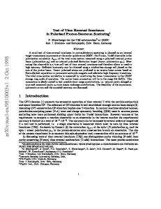
List of Figures 2.1 Feynman diagram for N ! X . : : : : : : : : : : : : : : : : : : : : : :

4

2.2 Feynman diagram for l + N ! l0 + X . : : : : : : : : : : : : : : : : : : :

7

2.3 Forward amplitude for virtual photon nucleon scattering. : : : : : : : : :

7

2.4 Feynman diagram for Quark Parton Model contribution to the forward scattering amplitude. : : : : : : : : : : : : : : : : : : : : : : : : : : : : :

9

2.5 Feynman diagrams for leading order QCD radiative processes contributing to virtual photon-nucleon scattering. a) Initial state gluon radiation. b) Final state gluon radiation. c) photon-gluon fusion to qq. : : : : : : : : : 13 2.6 a) Multiple gluon radiation Feynman diagram contributing to the N cross-section. b) Corresponding 'ladder diagram' contributing to the

N ! N forward scattering amplitude. : : : : : : : : : : : : : : : : 17 2.7 Interference contribution to the photon-quark cross-section. : : : : : : : : 18 2.8 Examples of diagrams contributing to higher twist = 4 processes. : : : : 18 3.1 Fixed target areas at Fermilab. : : : : : : : : : : : : : : : : : : : : : : : 27 3.2 New Muon beamline and the E665 beam spectrometer. : : : : : : : : : : 28 3.3 Frontal view of the run90/91 target assembly. : : : : : : : : : : : : : : : 30 3.4 Lateral view of a cryogenic liquid target vessel. : : : : : : : : : : : : : : : 31 xvi

3.5 The E665 forward spectrometer and muon detector. : : : : : : : : : : : : 33 3.6 A frontal view of the calorimeter showing the four \half" regions producing signals for the calorimeter trigger. : : : : : : : : : : : : : : : : : : : : 41 4.1 A ow chart indicating the connection between the structure functions and the measured muon distributions. : : : : : : : : : : : : : : : : : : : 47 5.1 Track parameter comparisons between data and Monte Carlo. : : : : : : 58 5.2 Positions of tracks at various chambers, for data and Monte Carlo. : : : : 59 5.3 Positions of tracks at various chambers, for data and Monte Carlo. : : : : 60 5.4 Number of detector hits on a track, for data and Monte Carlo. The sample consists of scattered muons and hadrons in inelastic scatters. In the pro le histograms on the right, the 'error bar' indicates the spread (not error on the mean). : : : : : : : : : : : : : : : : : : : : : : : : : : : 69 5.5 Number of detector hits on a track, for data and Monte Carlo. The sample consists of scattered muons and hadrons in inelastic scatters. In the pro le histograms on the right, the 'error bar' indicates the spread (not error on the mean). : : : : : : : : : : : : : : : : : : : : : : : : : : : 70 5.6 Overall eciency of identifying single halo tracks as muons, versus horizontal and vertical coordinate. : : : : : : : : : : : : : : : : : : : : : : : : 71 5.7 2 probability vs 2 of match between single forward spectrometer tracks and single muon projections. The position and slope parameters in each view are shown separately. This is a low momentum muon sample. : : : : 73 5.8 2 probability vs 2 of match between single forward spectrometer tracks and single muon projections. The position and slope parameters in each view are shown separately. This is a high momentum muon sample. : : : 74 5.9 number of detector hits on a track, for data and Monte Carlo. The sample consists of straight-through beams. : : : : : : : : : : : : : : : : : : : : : 76 5.10 Run dependence of muon nding eciency for data and Monte Carlo. : : 77 xvii

5.11 Forward spectrometer muon nding eciency for data. The eciency is shown as a function of the nearest occupied bucket in time. There are no 'out-of-time' beams in the Monte Carlo. : : : : : : : : : : : : : : : : : : 78 5.12 Forward spectrometer muon nding eciency for two-beam data events, and one-beam Monte Carlo events. The eciency is shown as a function of the position of one of the beams at the target. : : : : : : : : : : : : : : 79 5.13 PC and PCF segment nding eciency in straight-through beam data for various run blocks. The data at run 21840 were collected at low intensity. 80 5.14 Small Angle Trigger event distributions of Calorimeter Zflow . (a) Monte Carlo  , e sample. (b) Monte Carlo bremsstrahlung sample. (c) Monte Carlo sample of hadronic scatters. (d) Inclusive data sample. The arrow indicates the cut used to isolate hadronic scatters from the electromagnetic events. : : : : : : : : : : : : : : : : : : : : : : : : : : : : : : : : : 85 5.15 Average multiplicity vs log10Q2 in W bins, for Data and Monte Carlo. Hadronic scatters selected using the calorimeter are used. Only SATPS and SVS triggers are included. The average multiplicity is seen to be nearly independent of Q2. : : : : : : : : : : : : : : : : : : : : : : : : : : 86 5.16 Average multiplicity vs log10W in Q2 bins, for Data and Monte Carlo. Hadronic scatters selected using the calorimeter are used. Only SATPS and SVS triggers are included. The average multiplicity has a linear dependence on log10W . : : : : : : : : : : : : : : : : : : : : : : : : : : : 88 5.17 Average multiplicity vs log10W for all Q2, for Data and Monte Carlo. Hadronic scatters selected using the calorimeter are used. Only SATPS and SVS triggers are included. a) The average multiplicity in the data is higher by 8% than in the Monte Carlo, for any W . b) Monte Carlo corrected by scaling multiplicity by 1.08. : : : : : : : : : : : : : : : : : : 89 5.18 Normalized multiplicity distributions in W bins, for Data and Monte Carlo. Each distribution has been normalized to integrate to unity. Hadronic scatters selected using the calorimeter are used. Only SATPS and SVS triggers are included. The Monte Carlo multiplicity has been multiplied by 1.08, giving a good match with the data. : : : : : : : : : : 90 5.19 Normalized event distributions obtained from the data for the CAL, SATPS, SAT and SVS triggers. Each distribution is normalized to integrate to unity. : : : : : : : : : : : : : : : : : : : : : : : : : : : : : : : : 92 xviii

5.20 Normalized event distributions for the muon scattering angle obtained from the data for the CAL, SATPS, SAT and SVS triggers. Each distribution is normalized to integrate to unity. : : : : : : : : : : : : : : : : : 93 5.21 Multiplicity dependence of the muon reconstruction eciency measured from the data, and the corresponding Monte Carlo prediction. CAL and SATPS trigger samples are shown here. The curves are second-order polynomial ts and the t parameters described in the text are shown. : 95 5.22 Multiplicity dependence of the muon reconstruction eciency measured from the data, and the corresponding Monte Carlo prediction. SAT and SVS trigger samples are shown here. The curves are second-order polynomial ts and the t parameters described in the text are shown. : : : 96 5.23 Multiplicity dependence of the muon reconstruction eciency measured from the data, compared with the corresponding Monte Carlo prediction. CAL and SATPS trigger samples are shown here. The curves are the second-order polynomial ts described in the text and shown in the preceeding gures. : : : : : : : : : : : : : : : : : : : : : : : : : : : : : : 97 5.24 Multiplicity dependence of the muon reconstruction eciency measured from the data, compared with the corresponding Monte Carlo prediction. SAT and SVS trigger samples are shown here. The curves are the secondorder polynomial ts described in the text and shown in the preceeding gures. : : : : : : : : : : : : : : : : : : : : : : : : : : : : : : : : : : : : 98 5.25 Dierence in the multiplicity dependence of the muon reconstruction ef ciency measured from the CAL and SAT data, and the SVS and SAT data respectively. The lines show the t to a constant. : : : : : : : : : : 99 5.26 Dierence in the multiplicity dependence of the muon reconstruction eciency measured from the CAL and SAT Monte Carlo, and the SVS and SAT Monte Carlo respectively. The lines show the t to a constant. : : 99 5.27 Multiplicity dependence of the muon reconstruction eciency measured from the data, compared with the prediction of the nal Monte Carlo. CAL and SATPS trigger samples are shown here. : : : : : : : : : : : : : 100 5.28 Multiplicity dependence of the muon reconstruction eciency measured from the data, compared with the prediction of the nal Monte Carlo. SAT and SVS trigger samples are shown here. : : : : : : : : : : : : : : : 101 xix

5.29 DCA-DCB-PSA eciency of contributing to the scattered muon track, measured from the data using PC-PCF tracks. The eciency is plotted vs the track coordinates at DCA and DCB respectively. : : : : : : : : : : 104 5.30 DCA-DCB-PSA eciency of contributing to the scattered muon track, measured from the Monte Carlo using PC-PCF tracks. The eciency is plotted vs the track coordinates at DCA and DCB respectively. : : : : : 105 5.31 DCA-DCB-PSA eciency of contributing to the scattered muon track, measured from the data following cuts to eliminate dead regions. The eciency is plotted vs the track coordinate at DCA : : : : : : : : : : : : 106 5.32 DCA-DCB-PSA eciency of contributing to the scattered muon track, measured from the Monte Carlo following cuts to eliminate dead regions. The eciency is plotted vs the track coordinate at DCA. : : : : : : : : : 107 5.33 DCA-DCB-PSA eciency of contributing to the scattered muon track, measured from the data following cuts to eliminate dead regions. The eciency is plotted vs the track coordinate at DCB : : : : : : : : : : : : 108 5.34 DCA-DCB-PSA eciency of contributing to the scattered muon track, measured from the Monte Carlo following cuts to eliminate dead regions. The eciency is plotted vs the track coordinate at DCB. : : : : : : : : : 109 5.35 Comparison between data and Monte Carlo distributions for log10 (scattering angle), and scattered muon Y and Z coordinates at X = 4m. The individual distributions are normalized to integrate to unity, and superposed on the left. On the right the Data/MC ratio is shown. : : : : : : : 111 5.36 Muon reconstruction eciency predicted by the Monte Carlo. : : : : : : 112 5.37 Muon reconstruction eciency, including the DC-PSA acceptance, predicted by the Monte Carlo. : : : : : : : : : : : : : : : : : : : : : : : : : 113 5.38 Muon reconstruction eciency predicted by the Monte Carlo. The eciency is shown in two dimensions. : : : : : : : : : : : : : : : : : : : : : 114 5.39 Muon reconstruction eciency, including the DC-PSA acceptance, predicted by the Monte Carlo. The eciency is shown in two dimensions. : 115 6.1 Schematic diagram of the SAT. : : : : : : : : : : : : : : : : : : : : : : : 117 xx

6.2 Ineciency of RSAT simulation applied to RSAT and SAT triggers, as a function of run number. The lower histogram shows the dierence in the ineciencies for the two triggers. : : : : : : : : : : : : : : : : : : : : : : 120 6.3 Ineciency of SAT simulation to match the SAT hardware trigger, using all physics triggers as a study sample. : : : : : : : : : : : : : : : : : : : : 121 6.4 Model of the muon as it emerges from the hadron absorber and intersects the plane of the veto counter. : : : : : : : : : : : : : : : : : : : : : : : : 126 6.5 Contours of equal d and , which are the distance from the hodoscope and the angle subtended by the hodoscope. : : : : : : : : : : : : : : : : 128 6.6 SMS veto probability measured using Calorimeter trigger data. : : : : : 129 6.7 SMS veto probability for Monte Carlo events satisfying Calorimeter trigger simulation. : : : : : : : : : : : : : : : : : : : : : : : : : : : : : : : : 131 6.8 Dierence beween SMS veto probability measured from data and Monte Carlo. : : : : : : : : : : : : : : : : : : : : : : : : : : : : : : : : : : : : : 132 6.9 Dierence beween SMS veto probability measured from data and Monte Carlo. : : : : : : : : : : : : : : : : : : : : : : : : : : : : : : : : : : : : : 133 6.10 SSA Z hodoscope veto rate measured from the data, excluding e elastic scatters. : : : : : : : : : : : : : : : : : : : : : : : : : : : : : : : : : : : : 135 6.11 A cartoon depicting the nal state particles produced by the apparent virtual photon, in relation to the SSA veto hodoscope. : : : : : : : : : : 135 6.12 SSA Z hodoscope veto rate measured from the data, compared to the Monte Carlo prediction, using separate SATPS and LAT samples. : : : 138 6.13 SSA Z hodoscope veto rate measured from the data, compared to the Monte Carlo prediction, using separate SATPS and LAT samples. : : : 139 6.14 SSA Z hodoscope veto rate measured from the data, compared to the Monte Carlo prediction, using separate SATPS and LAT samples. : : : 140 6.15 SSA Z hodoscope veto rate measured from the data, compared to the Monte Carlo prediction, using separate SATPS and LAT samples. : : : 141 xxi

6.16 SSA Z hodoscope veto rate measured from the data, compared to the Monte Carlo prediction, using separate SATPS and LAT samples. : : : 142 6.17 SAT eciency vs kinematic variables, predicted by Monte Carlo. : : : : : 143 6.18 SAT eciency vs kinematic variables, predicted by Monte Carlo. A geometrical cut has been made around the SMS and SSA edges on the underlying muon distribution before the eciency is computed. : : : : : 144 6.19 SAT eciency vs kinematic variables, predicted by Monte Carlo. : : : : : 145 6.20 SAT eciency vs kinematic variables, predicted by Monte Carlo. A geometrical cut has been made around the SMS and SSA edges on the underlying muon distribution before the eciency is computed. : : : : : 145 7.1 Dierence ( ) between momenta of straight-through beams as measured by the beam and forward spectrometers. The mean dierence is shown for dierent run blocks, with the errors on the mean values. : : : : : : : : 150 7.2 Dierence ( ) between momenta of straight-through beams as measured by the beam and forward spectrometers. The upper plot is obtained from the data and the lower from the Monte Carlo. The curves are Gaussian ts to the distributions. : : : : : : : : : : : : : : : : : : : : : : : : : : : 151 7.3 log10xBj for data events passing the e selection. The curve is a sum of two Gaussians tted to the data. The t parameters are described in the text. : : : : : : : : : : : : : : : : : : : : : : : : : : : : : : : : : : : : : : 152 7.4 The  invariant mass distribution for V 0 vertices that pass the Ks0 selection. The curve is the sum of two Gaussians and a polynomial tted to the data. The t parameters are described in the text. : : : : : : : : 154 7.5  for straight-through beams normalized to the calculated error  . The data and Monte Carlo results are shown : : : : : : : : : : : : : : : : : : 156 7.6 log10Q2 and log10scat event distributions for straight-through beams, for Data and Monte Carlo. : : : : : : : : : : : : : : : : : : : : : : : : : : : 157

xxii

7.7 Distribution of the normalized error on reconstructed xBj for data and Monte Carlo events passing the e selection. xBj is the expected error calculated by the track- tting program. The curve is a sum of two Gaussians tted to the distribution. The parameter P3 is the r.m.s. of the main peak. : : : : : : : : : : : : : : : : : : : : : : : : : : : : : : : : : : : 159 7.8 Dierence between the generated (true) and the reconstructed kinematics, as a function of kinematics. The size of the 'error bar' shows the r.m.s. of the dierence in each bin. : : : : : : : : : : : : : : : : : : : : : : : : 160 7.9 Distributions of generated (true) and resolution-smeared kinematics for hydrogen. The distributions are very similar for high  and all Q2. : : : 162 7.10 Smearing correction for hydrogen and deuterium. : : : : : : : : : : : : : 163 8.1 Lowest order diagrams for real photon emission o the incoming and outgoing lepton legs. These are included in the calculated radiative correction. For soft photon emission, higher order diagrams are also summed. 167 8.2 Lowest order corrections to the Born diagram included in the calculated radiative correction. a) Virtual Z 0 exchange and Z interference is included in the radiative correction. b) Lepton vertex correction. c) Vacuum polarization, including e; ;  and quark loops. : : : : : : : : : : : : 167 8.3 Diagrams not included in the calculated radiative corrections. a) & b) hadron corrections, which by de nition are part of the hadron structure functions. c) Two photon exchange. : : : : : : : : : : : : : : : : : : : : 168 8.4 Calculated radiative correction for proton and deuteron, shown as a function of log10Q2(GeV 2) in bins of xBj . : : : : : : : : : : : : : : : : : : : : 171 8.5 Calculated radiative correction for proton and deuteron, shown as a function of log10Q2(GeV 2) in bins of xBj . : : : : : : : : : : : : : : : : : : : : 172 8.6 Calculated radiative correction for proton and deuteron, shown as a function of log10xBj in bins of Q2(GeV 2). : : : : : : : : : : : : : : : : : : : : 173 8.7 Calculated radiative correction for proton and deuteron, shown as a function of log10xBj in bins of Q2(GeV 2). : : : : : : : : : : : : : : : : : : : : 174

xxiii

9.1 Run dependence of the average trigger time (in ns) for various triggers. The time measurement involves an arbitrary oset. The CAL trigger was not installed in the early part of the run. : : : : : : : : : : : : : : : : : : 177 9.2 Run dependence of the SSA and SMS latching eciencies, as measured by the trigger element simulation software applied to RSAT triggers. For these events these elements should always be hit by the beam muon. : : : 178 9.3 Position distributions of RSAT beam tracks, compared for Data and Monte Carlo. : : : : : : : : : : : : : : : : : : : : : : : : : : : : : : : : : 180 9.4 Position, energy and curvature error distributions of RSAT beam tracks, compared for Data and Monte Carlo. : : : : : : : : : : : : : : : : : : : : 181 9.5 Geometry of cryogenic target vessel. : : : : : : : : : : : : : : : : : : : : : 183 10.1 Final Data-Monte Carlo comparisons of inclusive distributions. The distributions are normalized to integrate to unity before the comparison. The data and Monte Carlo distributions are superimposed on the left, and the data/MC ratio is shown on the right. Escat is the scattered muon energy, the other variables have their usual meaning. : : : : : : : : : : : 197 10.2 Final Data-Monte Carlo comparisons of inclusive distributions. The distributions are normalized to integrate to unity before the comparison. The data and Monte Carlo distributions are superimposed on the left, and the data/MC ratio is shown on the right.  is the muon scattering angle in radians, the other variables have their usual meaning. : : : : : 198 10.3 Final Data-Monte Carlo comparisons of inclusive distributions. The distributions are normalized to integrate to unity before the comparison. The data and Monte Carlo distributions are superimposed on the left, and the data/MC ratio is shown on the right. Y and Z are the transverse coordinates of the reconstructed scattered muon at the longitudinal position X = 4m, which is just downstream of the CCM magnet.  is the azimuthal angle of the muon scatter in radians. : : : : : : : : : : : : : : 199 10.4 proton F2 vs Q2(GeV 2) in xBj bins. : : : : : : : : : : : : : : : : : : : : : 202 10.5 deuteron F2 vs Q2(GeV 2) in xBj bins. : : : : : : : : : : : : : : : : : : : : 203 10.6 proton F2 vs xBj in Q2(GeV 2) bins. : : : : : : : : : : : : : : : : : : : : : 204 xxiv

10.7 deuteron F2 vs xBj in Q2(GeV 2) bins. : : : : : : : : : : : : : : : : : : : : 205 10.8 proton F2 vs Q2(GeV 2) in xBj bins, with curves showing the t to the data and the global F2 parametrization of appendix B. : : : : : : : : : : 206 10.9 deuteron F2 vs Q2(GeV 2) in xBj bins, with curves showing the t to the data and the global F2 parametrization of appendix B. : : : : : : : : : : 207 10.10proton F2 vs xBj in Q2(GeV 2) bins, with curves showing the t to the data and the global F2 parametrization of appendix B. : : : : : : : : : : 208 10.11deuteron F2 vs xBj in Q2(GeV 2) bins, with curves showing the t to the data and the global F2 parametrization of appendix B. : : : : : : : : : : 209 10.12Linear ts to lnF2 vs lnQ2 at xed x for proton. P2 is the slope. : : : : : 210 10.13Linear ts to lnF2 vs lnQ2 at xed x for proton. P2 is the slope. : : : : : 211 10.14Linear ts to lnF2 vs lnQ2 at xed x for proton. P2 is the slope. : : : : : 212 10.15Linear ts to lnF2 vs lnQ2 at xed x for deuteron. P2 is the slope. : : : : 213 10.16Linear ts to lnF2 vs lnQ2 at xed x for deuteron. P2 is the slope. : : : : 214 10.17Linear ts to lnF2 vs lnQ2 at xed x for deuteron. P2 is the slope. : : : : 215 10.18Logarithmic derivative of F2 with respect to Q2 (@lnF2=@lnQ2) at xed x, shown vs x for proton and deuteron. The photoproduction limit derived from real photon-proton cross-section measurements is also shown. : : : 216 10.19Linear ts to lnF2 vs lnx at xed Q2(GeV 2) for proton. P2 is the slope. : 217 10.20Linear ts to lnF2 vs lnx at xed Q2(GeV 2) for proton. P2 is the slope. : 218 10.21Linear ts to lnF2 vs lnx at xed Q2(GeV 2) for proton. P2 is the slope. : 219 10.22Linear ts to lnF2 vs lnx at xed Q2(GeV 2) for deuteron. P2 is the slope. 220 10.23Linear ts to lnF2 vs lnx at xed Q2(GeV 2) for deuteron. P2 is the slope. 221 10.24Linear ts to lnF2 vs lnx at xed Q2(GeV 2) for deuteron. P2 is the slope. 222 xxv

10.25Logarithmic derivative of F2 with respect to x (@lnF2=@lnx) at xed Q2, shown vs Q2 for proton and deuteron. The photoproduction limit derived from real photon-proton cross-section measurements is also shown, and the typical slope measured with the high Q2 HERA data is indicated. : : 223 10.26The deuteron-to-proton structure function ratio, measured by taking the ratio of the absolute structure functions in this analysis, and by an independent 'direct' analysis of the ratio. : : : : : : : : : : : : : : : : : : : : 224 11.1 proton F2 from E665 and NMC over-plotted vs Q2 in x bins. In certain x bins one of the two experiments has multiple data points because the actual binning in x is narrower. In these cases all the data points falling in those bins are shown. : : : : : : : : : : : : : : : : : : : : : : : : : : : 231 11.2 deuteron F2 from E665 and NMC over-plotted vs Q2 in x bins. In certain x bins one of the two experiments has multiple data points because the actual binning in x is narrower. In these cases all the data points falling in those bins are shown. : : : : : : : : : : : : : : : : : : : : : : : : : : : 232 11.3 proton F2 vs Q2(GeV 2) in xBj bins, from E665 and ZEUS. The BadelekKwiecinski (BK) model is also shown. : : : : : : : : : : : : : : : : : : : 233 11.4 proton F2 vs Q2(GeV 2) in xBj bins, with curves showing the calculation of GRV, CTEQ3 and the unmodi ed MRS(A). : : : : : : : : : : : : : : : 235 11.5 deuteron F2 vs Q2(GeV 2) in xBj bins, with curves showing the calculation of GRV, CTEQ3 and the unmodi ed MRS(A). : : : : : : : : : : : : : : : 236 11.6 proton F2 vs Q2(GeV 2) in xBj bins, with curves showing the calculation of Donnachie-Landsho, Badelek-Kwiecinski and the modi ed MRS(A). : 237 11.7 deuteron F2 vs Q2(GeV 2) in xBj bins, with curves showing the calculation of Donnachie-Landsho, Badelek-Kwiecinski and the modi ed MRS(A). : 238 11.8 proton F2 vs xBj in Q2(GeV 2) bins, with curves showing the calculation of GRV, CTEQ3 and the unmodi ed MRS(A). : : : : : : : : : : : : : : : 239 11.9 deuteron F2 vs xBj in Q2(GeV 2) bins, with curves showing the calculation of GRV, CTEQ3 and the unmodi ed MRS(A). : : : : : : : : : : : : : : : 240

xxvi

11.10proton F2 vs xBj in Q2(GeV 2) bins, with curves showing the calculation of Donnachie-Landsho, Badelek-Kwiecinski and the modi ed MRS(A). : 241 11.11deuteron F2 vs xBj in Q2(GeV 2) bins, with curves showing the calculation of Donnachie-Landsho, Badelek-Kwiecinski and the modi ed MRS(A). : 242 11.12Logarithmic derivative of F2 with respect to Q2 at xed x, shown vs x for proton and deuteron. The photoproduction limit derived from real photon-proton cross-section measurements is also shown. The data are compared with the Donnachie-Landsho model. : : : : : : : : : : : : : : 243 11.13Q2 dependence of the virtual photoabsorption cross-section for proton in W bins, compared with the Donnachie-Landsho model. : : : : : : : : : 244 11.14Q2 dependence of the virtual photoabsorption cross-section for deuteron in W bins, compared with the Donnachie-Landsho model. : : : : : : : : 245 B.1 Fp2 in the resonance region for various Q2. : : : : : : : : : : : : : : : : : : 279 B.2 Fp2 in the low W region for various Q2. : : : : : : : : : : : : : : : : : : : 280 B.3 Fp2 in the intermediate W region for various Q2. : : : : : : : : : : : : : : 281 B.4 Fp2 for various Q2. : : : : : : : : : : : : : : : : : : : : : : : : : : : : : : : 282 C.1 Fortran code used to evaluate Rslac and the error on it.

: : : : : : : : : 285

C.2 Parametrization of Rslac and error, plotted vs log10x in Q2 bins. : : : : : 286 C.3 Parametrization of Rslac and error, plotted vs log10x in Q2 bins. : : : : : 287 C.4 Parametrization of Rslac and error, plotted vs log10Q2 in x bins. : : : : : 288 C.5 Parametrization of Rslac and error, plotted vs log10Q2 in x bins. : : : : : 289 C.6 Parametrization of RQCD in Fortran : : : : : : : : : : : : : : : : : : : : : 290 D.1 a) X distribution of primary vertex in meters. b) distance (in meters) between calorimeter cluster and negative track impact point on calorimeter.293 xxvii

D.2 log10xBj distribution following calorimeter and track multiplicity cuts. : : 293 D.3 a) Ztrack  Ptrack = distribution of  , e candidates. b) normalized error on reconstructed xBj . : : : : : : : : : : : : : : : : : : : : : : : : : : : : 294 D.4 a) log10xBj vs Ztrack distribution of  , e candidates. b) normalized error on reconstructed xBj of nal calibration sample. : : : : : : : : : : : : : 295 D.5 Distributions of the nal calibration sample. top row)  and Ptrack . middle row) Y and Z position of the calorimeter cluster in meters. bottom row) mean cluster position in Y and Z (meters) as a function of calibration energy. : : : : : : : : : : : : : : : : : : : : : : : : : : : : : : : : : : : : 296 D.6 Distributions of Zcluster uncorrected for non-linearities. The errors on the Zcluster vs Ecalib plot show the spread on Zcluster and not the error on the mean. : : : : : : : : : : : : : : : : : : : : : : : : : : : : : : : : : : : : : 299 D.7 Distributions of Zcluster corrected for non-linearities using the Ecluster parameterization. : : : : : : : : : : : : : : : : : : : : : : : : : : : : : : : : 300 D.8 Distributions of Zcluster corrected for non-linearities using the Ecalib parameterization. : : : : : : : : : : : : : : : : : : : : : : : : : : : : : : : : 302 D.9 Distributions of Zcluster for clusters simulated using the Ecalib parameterization and corrected using the Ecluster parameterization. : : : : : : : : : 303

xxviii

Chapter 1 Introduction Scattering experiments have proven to be a very eective technique for probing the structure of matter. The large angle scattering of  particles o a gold foil led Rutherford to conjecture that the bulk of the mass of the atom must be contained in a very small, positively charged nucleus of the atom. The momenta of the  particles varied between 4 and 9 MeV. This, and the angular distribution of the scattered  particles, provided the estimate that the nuclear radius was less than 10,12 cm. The formulation of this scattering process was based on the Coulomb force law. At these distances the electromagnetic interaction dominates, simplifying the interpretation of the results of the scattering experiments. But the ability of  particles to probe smaller distances was hampered by the fact the interaction ceased to be purely electromagnetic. At short distances the  particle starts to interact through the strong interaction with the nucleus. Charged lepton scattering promised to be an eective technique of probing the internal structure of nuclear matter, since the interaction of the probe is purely electromagnetic. In the 1950's, starting with electron scattering experiments at SLAC [1], experiments were performed at Darmstadt, Orsay, Yale and the CEA to measure the charge distributions of various nuclei. At the energies available, the experiments were restricted to elastic scattering or excitation of the low-lying resonances. The measured elastic form factors fall rapidly with increasing 4-momentum transferred, indicating that the charge distribution in nuclei is spatially extended and smoothly varying (i.e. there is no hard core in the nucleus). As higher energy electron beams became available at SLAC in the late 1960's, inelastic scattering experiments could be performed. These experiments [2] showed that, at large 4-momentum transfers, the inelastic nucleon structure functions were independent of any dimensioned quantity, a phenomenon known as scal1

2 ing. This result was interpreted as evidence for the existence of point-like constituents in the nucleons [3], as this behavior was predicted on the basis of current algebra [4]. These \partons" are now associated with quarks [5], which were rst introduced to describe hadron spectroscopy [6, 7]. Higher energy electron beams became dicult to produce as electrons, being light, are good at losing energy through synchrotron radiation. Muons became a natural choice as high energy charged lepton probes. The 1970's and 1980's saw the development of the CHIO, EMC, BCDMS, NMC and E665 muon scattering experiments, and the ep collider HERA at DESY [8, 9, 10, 11, 12, 13, 14]. In the meantime, the quarkparton model developed into a dynamic gauge eld theory of interactions called Quantum Chromo-Dynamics (QCD). This theory has been quite eective in making perturbative calculations of the short distance behavior of quark interactions. In particular, QCD predicted a pattern of scaling violations of the inelastic structure functions at large 4momentum transfers, which has been con rmed by the high energy muon experiments and the HERA experiments. However, at low values of 4-momentum transfers, the perturbative QCD framework breaks down. Real photoproduction measurements at high energy reveal the hadronic nature of the photon. This behavior is dierent from the point-like photon-parton interactions manifested at large 4-momentum transfers. The transition from the regime of perturbative QCD to the domain of the hadronic photon must involve some change in the nature of photon-hadron interactions as a function of 4-momentum transfer. The experiment 665 provides a wide range of energy and 4-momentum transfer and thus an opportunity to understand the nature of this transition. This work presents the measurement of the proton and deuteron structure functions at E665, using the data taken during 1991-92. In the next chapter, we discuss the theory and phenomenology of the photon-nucleon interaction. In chapter 3, a brief description of the experimental apparatus will be given. In chapter 4, the structure function measurement technique will be described. In the following chapters, detailed discussions will be provided of the analysis. The analysis issues are the estimation of the muon reconstruction and triggering eciencies, the detector calibration and resolution, the radiative corrections and the luminosity measurement. In chapter 10, the results and the systematic uncertainties will be presented. The results will be compared with measurements from other experiments and with theoretical models in chapter 11. Throughout this thesis, we use a right-handed coordinate system, where the x-axis points along the nominal beam direction (north). The y-axis points to the west and the z-axis points upwards. Hodoscopes and wire chambers are labelled by the coordinate they measure.

Chapter 2 Virtual and Real Photon - Nucleon Interactions The reason that charged lepton scattering is such an eective tool to probe nucleon structure is twofold. Firstly, the coupling of the photon to the lepton is calculable in terms of Quantum Electro-Dynamics (QED). The electromagnetic coupling constant being small, allows the perturbative techniques of QED to be applied and the radiative corrections to the Born diagram to be calculated. Secondly, the single photon exchange approximation allows the diagram to be factorized, i.e. separated into the lepton vertex and the hadron vertex. The hadron vertex can then be expressed in general without regard to the source of the virtual photon. Once the general form of the photon-nucleon vertex is written down, the rules of QED allow us to write down the photoproduction cross-section, and the lepto-production cross-sections assuming single photon exchange. Hence let us start with the formulation of the photon-nucleon interaction.

2.1 Formulation of the Photon-Nucleon Interaction 2.1.1 Photon-Nucleon Vertex and the Hadron Tensor The interaction of a photon of 4-momentum q and polarization  with a nucleon of 4-momentum p to produce a nal state X is depicted in gure 2.1. The electromagnetic current of the nucleon A coupling to the photon may be written as the matrix element of the current operator J between the initial and nal hadronic 3

4 γ∗ ε

q

X

p N

Figure 2.1: Feynman diagram for N ! X . states:

A = hX jJ jN i The cross-section is given in terms of the hadronic tensor W , de ned by X W = 12 AA (2)34(p + q , pX ) X

(2.1) (2.2)

In the case of the electromagnetic interaction the general form of W is constrained by parity conservation and gauge invariance. Parity conservation forces W to be symmetric. Since the photon tensor and the lepton tensor (discussed below) are symmetric, only the symmetric parts of W contribute to the photoproduction and leptoproduction cross-sections. Gauge invariance forces the conservation of the electromagnetic current qA = 0 = qW . For an unpolarized nucleon the most general Lorentz invariant expression for W can be written as W2 [(p , p:q q )(p , p:q q )] W = W1(,g + qqq2  ) + M (2.3) 2  q2   q2  where the \structure functions" W1 and W2 are Lorentz invariant functions of q2 and  ( p:q M ), and M is the nucleon mass (see discussion in [15]). The structure functions are often rede ned in the following way:

F1 = MW1

(2.4)

F2 = W2

(2.5)

5

2.1.2 Photon Tensor Let us now turn to the photon. Throughout this thesis we work in the Lorentz gauge, so that q: = 0 where  is the photon polarization vector. In general the photon may be described by a superposition of three polarization states: left- and right-transverse photons (helicity 1) and longitudinal-scalar photons (helicity 0). For a space-like photon moving along the z-axis the 4-momentum may be written as

q

q

= (; 0; 0; Q2 +  2)

(2.6)

The conditions q: = 0 and ji :j j = ij then de ne the polarization vectors for the three states to be: (1) =  p1 (0; 1; {; 0) (2.7) 2 and q (0) = p1Q2 ( Q2 +  2; 0; 0;  ) (2.8) where Q2 = ,q2 (see discussion in [15, 16]).

2.1.3 Photoabsorption Cross-sections Since parity is conserved and the target is unpolarized there are two independent photoabsorption cross-sections, S for the scalar photons and T = (+ + ,)=2 for the transverse photons. The photoabsorption cross-sections are obtained by contracting the appropriate photon polarization vectors with the hadronic tensor W .

;S = 4K y1;0W 1;0 2

where K is the photon ux. This yields the following relationships [15] W1 = 4K2 T 2 W2 = 4K2 (T + S ) Q2Q+  2 2 ) , 1 2 R = S = W (1 + W1 Q2 T

(2.9)

(2.10) (2.11) (2.12)

6

2.1.4 Leptoproduction Cross-sections The kinematics of the lepton-nucleon scattering are expressed in terms of the 4-momenta of the incoming lepton (k), the outgoing lepton (k0) and the target nucleon (p). The 4-momentum of the exchanged virtual photon is q = k , k0, and that of the hadronic nal state is pX . M is the rest mass of the target nucleon. The useful kinematic quantities are the following:

Q2 = ,q2  = p:q=M W 2 = (p + q)2 = p2X xBj  x = Q2=2p:q = Q2=2M yBj  y = M=p:k

(2.13) (2.14) (2.15) (2.16) (2.17)

In the laboratory frame in which the target is at rest,  reduces to the energy of the virtual photon (or the energy lost by the lepton), and yBj or y equals =E , where E is the energy of the incoming lepton. Using the Born diagram shown in gure 2.2, the leptoproduction cross-section may be written down in terms of W :

d2 = 2 L W  (2.18) d dE 0 Q4  where L is the lepton tensor calculated for the lepton-photon vertex [15]. This is completely calculable in QED and is identical in almost all respects for the electron and the muon, due to lepton universality. The dierence is only in mass of the lepton ml. L is given by: L = 2(k k0 + k0 k , (k:k0 , m2l )g ) (2.19) The lepton mass can usually be ignored at high energies1. This gives the following double dierential lepton-nucleon scattering cross-section [17], d2 = 2em (2W sin2  + W cos2  ) (2.20) 2 d dE 0 4E 2 sin4 2 1 2 2 where E 0 is the energy of the scattered lepton,  is the lepton scattering angle and

is the solid angle in the laboratory frame. The dierential cross-section may also be 1

except in the calculation of certain quantities like Q2 which could be small even at high energies.

7 expressed in terms of the following invariants: d21 = 42em F (x; Q2)[1 , y , Mxy + y2(1 + 4M 2x2=Q2) ] (2.21) d(Q2)dx Q4x 2 2E 2(1 + R(x; Q2)) where the single photon exchange cross-section is explicitly denoted. R, which is the ratio of scalar to transverse photon cross-sections de ned in equation 2.12, can also be de ned as 2 2 2 R = (1 + 4M2xFx =Q )F2 , 1 (2.22) 1

Thus we see that we need two functions, which we choose to be F2(x; Q2) and R(x; Q2), to describe the scattering of photons, electrons and muons o unpolarized nucleons. incident lepton µ

scattered lepton µ ’

k

k’

q

p

virtual photon γ∗

p X

hadronic final state X

target nucleon N

Figure 2.2: Feynman diagram for l + N ! l0 + X . γ∗

γ∗ q

q JJ(ξ) (ξ)

N

p

J(0) p

Figure 2.3: Forward amplitude for virtual photon nucleon scattering.

N

8

2.1.5 Optical Theorem We now turn our attention to the hadronic tensor W . As shown in gure 2.1 and equation 2.2, it represents the sum over all nal states produced in the interaction of the photon and the nucleon. Since the total probability is conserved, there must be a corresponding loss of intensity which the photon beam suers because of the scattering. The optical theorem (see discussion in [18]) shows that this loss is related to the imaginary part of the amplitude for photon-nucleon scattering in the forward direction. The Feynman diagram for this process is shown in gure 2.3. Based on the optical theorem, W may be written as (see discussion in [17])

Z d4 iq: X 1 W (p; q) = 4M 2 e < p; j[J(); J (0)]jp;  > 

(2.23)

Here p and q denote the 4-momenta of the target nucleon and the virtual photon respectively. jp;  > denotes the wavefunction of the nucleon, where  denotes its spin which is summed over. The commutator denotes the creation of the electromagnetic current at spacetime coordinate 0 and its annihilation at spacetime coordinate . The advantage of this formulation is that the total cross-section may be studied by understanding the forward scattering amplitude.

2.1.6 Operator Product Expansion For small spacetime separation , the bilocal operator may be expanded in the Wilson Operator Product Expansion [19] 2

!0 iT (J(); J (0)) ,!

1 X 1 X C;n(2 ; 2)1 : : : n O1


n (2 )

 =2 n=0

(2.24)

where T denotes the time-ordering operation. The coecients C;n are complex numbers, n being the spin of the operator O and  is called the \twist". It is the mass dimension of O minus its spin. As we shall see, it determines the singularity structure of the terms in the expansion as 2 ! 0. 2 is the renormalization point. In the operator product expansion, the long distance physics is absorbed into the operators O , while the coecients C;n contain the physics at short distances. The momentum cuto distinguishing between long and short distances is the renormalization scale 2, which occurs in both C;n and O , so that the total amplitude is independent of the arbitrary cuto.

9 The coecients C;n become singular as 2 ! 0. It can be shown [17] that 2 C;n(2 ; 2)  !0 ( 12 )1, 2 (2.25) so that the structure functions have the following form as 2 ! 0 (corresponding to Q2 ! 1) (2.26) W ! C;n(Q2; 2)On (2)x,n( Q12 ) 2 ,1 The On describe various components of the nucleon wavefunction, and the C;n(Q2; 2) describe the hard scattering of the photon o these components. The dominant contribution at high Q2 comes from the twist-2 component, and higher twist contributions are suppressed by powers of Q2 that increase with the twist.

2.2 Quark Parton Model (QPM) Taking the limit as Q2 ! 1 for xed x (known as the Bjorken limit), it has been shown [20] that the dominant contribution to the cross-section comes from the diagram shown in gure 2.4. This diagram is sometimes called the \handbag" diagram. It corresponds to the photon scattering incoherently o point-like constituents in the nucleon. The reason that this contribution dominates is as follows. In the Bjorken limit, the time scale associated with the scattering process becomes very small. A spatially extended charge distribution is unable to scatter the photon, because this would require some amount of time for the dierent parts of the charge cloud to communicate with each other. The shrinking time scale of the scatter leads us to the impulse approximation, in which the nucleon wavefunction appears \frozen" to the virtual photon. γ∗

N

γ∗

N

Figure 2.4: Feynman diagram for Quark Parton Model contribution to the forward scattering amplitude.

10 Since point-like particles do not have momentum dependent form factors, the structure functions in the Bjorken limit are expected to scale, i.e. they will not depend on any dimensional quantity. This is the statement of Bjorken Scaling [4]. When the structure functions measured at SLAC in the early 1970's [2] showed approximate scaling behavior, this was in fact interpreted as evidence for the presence of point-like constituents in the nucleon [3]. The elastic scattering of the photon by a parton i carrying a momentum fraction xi of the nucleon, leads to the kinematic constraint that xBj = xi. That is to say, xBj measures the fractional momentum of the parton in the nucleon. This result is valid as long as the parton moves on the light-cone, i.e. it has no transverse momentum and is massless. The structure functions are then related to the number density and momentum density of the partons. Quarks had been invented to explain hadron spectroscopy [6, 7]. The combination of the parton model, and the properties of the quarks led to the hypothesis that quarks were the partons [5]. The Quark-Parton model explained most of the features of the measured structure functions in the early 1970's. The spin 1/2 nature of the quarks and the quark charge assignments led to the following relations:

F1(x) = F2(x) =

X e2q (x) i i i X e2xq (x) i

i

i

(2.27) (2.28)

where i labels the species of the quark, qi(x) is the number density of the quarks with momentum fraction x and ei is the electric charge of species i. The spin 1/2 nature of the quarks is re ected in the Callan-Gross [21] relation

F2(x) = 2xF1(x) (2.29) implying that R  0. This is because, as the spin 1/2 quark moving on the light cone absorbs the virtual photon and rebounds, its spin must ip in order to conserve its helicity. Therefore it absorbs one unit on angular momentum. By angular momentum conservation, the virtual photon must be transversely polarized, and a scalar virtual photon cannot be absorbed by the quark. The small value of R measured at SLAC supported the Quark-Parton Model.

2.2.1 Quantum Chromo-Dynamics Quantum Chromo-Dynamics (QCD) is a local gauge eld theory that attempts to describe the strong interactions between quarks. The gauge group is the non-Abelian

11 SU(3) group, and the generators of the gauge transformations are called gluons. Thus, we say that the quarks interact with each other through the exchange of gluons, and the QCD 'charge' possessed by the quarks is called color. The non-Abelian nature of SU(3) causes the gluons to couple to each other directly, i.e. the gluons are colored as well. This latter property proves crucial in the result that QCD is an asymptotically free theory [22, 23, 24]. As in QED, the eective coupling constant in QCD (s) is momentum-dependent due to the presence of vacuum uctuations. The fermion loops (quark loops in the case of QCD) in the gluon propagator have the eect of screening the color charge at large distances. The quark loops alone would cause s to reduce with increasing distance. However, the gluon loops have the eect of spreading out the color charge, so that a smaller net charge remains at small distances. In SU(3) with eight gluons, the gluon anti-screening eect wins over the screening eect of the quarks as long as the number of quark avors is less than 16 (based on the leading order calculation). Thus, s decreases at small distances, i.e. large momentum transfers. The leading order expression for s is [17] (2.30) s (Q2) = (11 , 2 N 4)ln(Q2=2) 3 f

where Q2 is the square of the 4-momentum transferred by the gluon, and Nf is the number of quark avors.  is the natural momentum scale that sets the magnitude of s, and it must be measured by experiment. As the leading order expression indicates, s(Q2) ! 0 as Q2 ! 1.

Asymptotic freedom provides the justi cation for the application of perturbative QCD techniques to the interactions of quarks and gluons in processes involving large momentum transfers. We shall now study the QCD radiative processes that aect the parton momentum densities inside the nucleon.

2.2.2 QCD Evolution of Structure Functions At high Q2 we may neglect the higher-twist contributions to the structure functions, so we will restrict our attention to the twist-2 contributions. In that case, the structure functions can still be expressed in terms of parton distributions. However, in the presence of QCD radiative eects, the parton distributions acquire an explicit momentum dependence. The study of these eects leads to the development of the QCD-improved parton model. At rst order in s, a quark or an antiquark may radiate a gluon, before or after absorbing the virtual photon. In addition, a gluon may split into a quark-antiquark pair,

12 and one of the pair may absorb the photon. These processes are shown in gure 2.5. The diagrams have divergences when the internal propagators become close to massshell. This situation occurs either when the radiation or the splitting is collinear with the incoming parton, or when one of the radiated partons becomes very soft. In addition to these diagrams, there are virtual gluon loops.The divergences in the soft virtual gluon diagrams serve to cancel the divergences in the soft real gluon emission, order by order in perturbation theory. The collinear divergences are removed by absorbing them into the de nition of the incoming parton. This introduces a renormalization scale . If the transverse momentum of the radiation is below this cuto, the contribution is absorbed into the rede nition of the parton distribution. For a transverse momentum larger than the cuto, the matrix element of the radiative diagram is explicitly carried through. Clearly, if all the diagrams were calculated to all orders in perturbation theory, absorbing a part of phase space into the de nition of the parton distribution and keeping the remainder of the phase space in the matrix element explicitly would make no dierence. So the exact answer will be independent of the renormalization scale . In practice, the calculations are not performed exactly to all orders. As a result of the approximate nature of the calculation, there is a renormalization scale dependence in the nal answer. One expects the renormalization scale dependence to reduce as higher order diagrams are calculated and better techniques are developed to sum up all the diagrams. The cross-section calculated from the radiative diagrams depends on the momentum scale of the process. This dependence comes from the virtuality of the internal propagators, and the phase space available for the radiated gluons or the qq produced in photon-gluon fusion. In addition, s is expected to vary with the momentum scale. One expects this scale to be set by the photon-parton center-of-mass energy. All the momentum scales can be related to each other through dimensionless variables. The general convention in inclusive scattering is to use the square of the 4-momentum of the photon, Q2, to represent the momentum scale of the scatter, while the dimensionless variables are either held xed or integrated out. The eld-theoretic calculations of these processes are given in [25, 26]. The AltarelliParisi (AP) evolution equations [27] for parton densities indicate how the eective parton densities change with the momentum scale of the scatter. As shown in gure 2.5, a parton with apparent momentum fraction x that scatters the photon may in fact be derived from a parton with higher momentum fraction y. The probability that a parton will split to produce another parton carrying a momentum fraction z of itself is called the \splitting function" and denoted by P (z). The AP evolution equations are written as:

dq(x; Q2) = s(Q2) Z 1 dy [q(y; Q2)P ( x ) + G(y; Q2)P ( x )] qq qG dlnQ2 2 x y y y Z 2 2 dG(x; Q ) = s(Q ) 1 dy [q(y; Q2)P ( x ) + G(y; Q2)P ( x )] Gq GG dlnQ2 2 y y y x

(2.31)

13

a)

b)

g γ∗

γ∗ q

q

g q

q

N

N

c)

γ∗ q

q

g

N

Figure 2.5: Feynman diagrams for leading order QCD radiative processes contributing to virtual photon-nucleon scattering. a) Initial state gluon radiation. b) Final state gluon radiation. c) photon-gluon fusion to qq.

14

q(x; Q2) is the quark density and G(x; Q2) is the gluon density. The change in the quark density is due to the splitting processes q ! gq and g ! qq. The gluon density changes due to the processes q ! qg and g ! gg. The interesting thing to note is that the change in the parton densities is logarithmic in Q2. This can be traced back to the integration of the matrix elements (shown in gure 2.5) over the available phase space for the radiated parton. The integrand has the form dp2t =p2t leading to a lnp2t dependence of the quark density. The maximum p2t of the nal state partons depends on the c.m.s. energy of the photon - initial parton system, which in turn can be related to Q2. The minimum p2t chosen in the integration corresponds precisely to the renormalization scale 2 mentioned earlier. Thus, for a set of de ned parton distributions at scale 2, the parton distributions relevant for hard scattering at a scale Q2 > 2 may be calculated using the evolution equations. For example, the structure function F2 may be related to the parton distributions observed in hard photon-parton scattering. There is some arbitrariness in de ning which parton actually scatters the photon. In a photon-gluon fusion event, should one think of the gluon as the scatterer or the quark coupling to the photon as the scatterer? This ambiguity leads to \scheme dependence" of the parton distributions. In the DIS scheme, the partons that scatter the photon are always de ned to be the quarks. In this scheme, F2 still has the same expression as in the Quark-Parton model

F2(x; Q2) =

X e2xq(x; Q2) i

(2.32)

where the sum is over all species of quarks and antiquarks. QCD radiation also plays a role in the determination of R. As noted earlier, in the Quark-Parton model the spin 1/2 quarks can only absorb transverse photons. However, if the quark were to radiate a real gluon carrying spin 1, the helicity of the virtual quark is ipped already. Therefore it can absorb a scalar photon and rebound with the appropriate helicity for an on-shell quark. Thus the ability to radiate gluons allows the quarks to absorb scalar photons and produce a contribution to R. The x dependence of the parton distributions (and hence the structure functions) is in uenced by the QCD radiative processes. The eect of these processes is to create partons carrying less momentum than the parent partons, since the QCD radiation carries away some of the momentum. This produces a pile-up of partons at low x and a depletion of partons at high x. Through the emission of multiple partons, QCD radiative processes play the dominant role in the determination of the x dependence of the structure functions. We will discuss this in the next section.

15

2.2.3 Low x Behavior of Structure Functions in QCD The splitting functions for a quark or a gluon to radiate a gluon, PGq (z) and PGG (z), behave as 1=z for small z. This is a re ection of the tendency of the matrix elements to diverge as the radiated gluon becomes soft. There is therefore a propensity to radiate multiple soft gluons, leading to diagrams such as shown in gure 2.6a. The corresponding diagram contributing to the forward scattering amplitude is shown in gure 2.6b. At low x such processes are expected to produce a pile-up of partons and hence a rapid rise in the structure functions as x falls. These diagrams are dicult to calculate because of the complexity of the multiparticle phase space. In the leading logarithm approximation, the total phase space is approximated by that part in which the transverse momenta of the radiated partons are ordered and the parton coupling to the photon has the maximum transverse momentum. At each order in perturbation theory this part of the phase space gives the dominant contribution, which upon integration gives a term like (slnQ2)n . In the double leading logarithmic approximation, one deals with the situation in which the longitudinal momenta of the radiated partons are also ordered such that the parton coupling to the photon has the minimum longitudinal momentum. This corresponds to the situation where the parton distribution at low x is being probed. At low x the gluon distribution becomes more singular than the quark distributions. If the quark distributions are ignored, the AP equation may be solved for the gluon distribution, with the result xG(x; t) = exp[(,2Ktlnx) 21 ] (2.33) lnQ2=2 ] and K = 24=(11 , 2N =3). This rapid increase in the gluon where t = ln[ lnQ 20 =2 f momentum density at small x is the result of taking the small x limit of the AP evolution equations in the double leading log approximation (DLLA) where ln(1=x), lnlnQ2=Q20  1. Relaxing the ordering of the radiated partons in transverse momentum introduces terms beyond leading order in lnQ2. The sum of the leading powers of ln(1=x) (and arbitrary powers of lnQ2) corresponds to the leading ln(1=x) approximation. In this approximation is obtained the Balitskij-Fadin-Kuraev-Lipatov (BFKL) solution (see discussion in [28]) for the parton densities, which rises at low x even more rapidly than the DLLA solution. For instance, the gluon density in the BFKL solution behaves as xG(x; Q2)  exp[(n0 , 1)ln(1=x)]  x,D (2.34) where D = (n0 , 1) = (3s =)4ln2  0:5. Therefore the small x behavior in the region where sln(1=x)  1 is singular xG(x; Q2)  x,0:5 (2.35)

16 This rapid rise in the number of partons at low x would eventually cause the virtual photon-nucleon cross-section to violate the Froissart2 bound. At very low x some new physics must enter to soften the singular asymptotic behavior of the parton distributions. The new ingredients are expected to be the self-interactions of the gluons, which will increase as the gluon density increases. The AP equations are modi ed to take into account the eect of gluon recombination in the nucleon, in terms of a two-gluon correlation function [29].

2.2.4 Transition to Low Q2 So far we have been discussing the behavior of the structure functions when Q2 is large enough that the nucleon can be considered an incoherent superposition of partons. We have ignored the interference contributions to the photon-quark cross-section, such as the one shown in gure 2.7. This diagram is sometimes called the \cat's ears" diagram. In contrast to the \handbag" diagram of gure 2.4, the \cat's ears" diagram corresponds to the outgoing photon being emitted from a dierent quark than the one that absorbed it. How can this happen? The two quarks must be correlated with each other, and the photon is scattering o a two-quark wavefunction inside the nucleon. The statement of Bjorken scaling is that the \cat's ears" diagram is heavily suppressed with respect to the \handbag" diagram. The reason for this may be understood as follows. We may look at the \cat's ears" diagram inpthe Breit frame without loss of generality. In this frame, the photon has 3-momentum Q2 and no energy. Therefore it transfers a 3-momentum p Q2 to the quark that absorbs it. The rst quark must somehow transfer this large momentum to the second quark so that it can emit the nal state photon. This transfer must occur through an internal propagator connecting the two, which must be o-shell by at least Q2. This is illustrated in gure 2.8a. So we expect that the \cat's ears" diagram is suppressed with respect to the \handbag" diagram by a power of Q,2. This is an example of a higher-twist process. Another example of a higher-twist process is shown in gure 2.8b, which may be interpreted as multiple interactions of the struck quark with other partons in the nucleon. Higher twist contributions have been studied in terms of multiparton distributions and the corresponding parton cross-sections [30]. An analysis of SLAC data on R = S 2 2 T at Q = 5GeV [31, 32] shows that twist-4 terms are required in addition to the leading twist (next-to-leading order QCD corrections included) plus consistent target mass corrections. Low Q2 data provides further opportunities to study higher twist processes. The Froissart bound is a consequence of unitarity and analyticity. It implies that, asymptotically, the total cross-sections cannot increase faster than ln2 s. See [28] for a review. 2

17

a)

γ∗

N

b)

N

γ∗

γ∗

N

Figure 2.6: a) Multiple gluon radiation Feynman diagram contributing to the N crosssection. b) Corresponding 'ladder diagram' contributing to the N ! N forward scattering amplitude.

18

γ∗

γ∗

Ν

Ν

Figure 2.7: Interference contribution to the photon-quark cross-section. a)

γ∗

γ∗

N

N

γ∗

γ∗

b)

N

N

Figure 2.8: Examples of diagrams contributing to higher twist = 4 processes.

19

2.3 Low Q2 Phenomenology In the preceeding discussions, we have treated the photon as a purely electromagnetic probe. Its interaction with the nucleon is understood in terms of its interaction with the charged quarks. The photon may scatter incoherently o a quark (quark parton model QPM), the struck quark may be derived by radiation from other quarks or gluons (QCDimproved parton model), and the struck quark may re-interact with other partons in the nucleon (higher twist eects). All the structure has been assigned to the nucleon and the photon has been considered a point particle. This approach was taken using the operator product expansion on the light cone, which is a kind of Taylor expansion that works well in the high Q2, high  limit. Another approach has evolved that examines the structure of the photon itself. Unlike the previous approach which worked best in the in nite-momentum frame (nucleon is on the light cone), the second approach examines the photon-nucleon scattering process in the frame in which the nucleon is at rest (referred to as the laboratory frame in xed-target experiments).

2.3.1 Hadronic Nature of the Photon In a relativistic quantum eld theory such as QED, a photon may uctuate into a particle-antiparticle pair. The physical photon state is a superposition of the bare (noninteracting) photon state and the particle-antiparticle state, since the interaction Hamiltonian causes a mixing between the latter two states. The particle-antiparticle state may be a lepton pair, or it may be quark-antiquark state which may evolve further. Since the leptons will have small cross-section to interact with the target nucleon, we will not consider them further. Using lowest order time independent perturbation theory, we may write (see discussion in [33]) 0 X j physical >= j bare > +pem jn > n

n

(2.36)

where the sum is over all hadronic states jn > that couple through the interaction Hamiltonian H 0 to the bare photon state j bare >.  is the energy of the photon and En is the energy of the hadronic state with invariant mass mn with 3-momentum equal to that of the photon. At high energy the energy dierence may be approximated,  , En ' (m2n + Q2)=2 , yielding X j physical >= j bare > +pem (m2 2+ Q2) jn >< njH 0j bare > (2.37) n n

20 As the energy increases the hadronic states become degenerate with the photon and degenerate state perturbation theory must be used. The amount of mixing between degenerate states is not suppressed by powers of the coupling constant, and the hadronic component of the physical photon can be quite large. The picture of the photon-nucleon interaction is that it proceeds through the interaction of the hadronic component of the photon with the nucleon.

2.3.2 Vector Meson Dominance (VMD) The spectrum of hadronic states jn > is limited to those sharing the same quantum numbers as the photon. The spectrum will be dominated by the low-mass vector mesons ; ! and  due to the large values of the mixing matrix elements for these states. Using the VMD model, the predicted form of the structure function F2 is [34] 2 X M 4  (W 2) v vN F2(Q2; W 2) = Q 2 4 v v (Q2 + Mv2)2

(2.38)

where the Q2 factor arises due to gauge invariance as will be shown below. The sum is carried out over the ; ! and  vector mesons, Mv is the mass of the vector meson, vN (W 2) is the meson-nucleon cross-section, and the denominator contains the vector meson propagator. v2 is the coupling of the photon to the vector meson and may be obtained from the measured leptonic width. The meson-nucleon cross-sections may be derived from the measured p and Kp total cross-sections. [34].

2.3.3 Real Photoproduction Limit of S and R Let us try to study the behavior of S as Q2 ! 0. The amplitude for the absorption of a helicity 0 photon is q 2 2 1 A(S ) = (0):A = Q ( Q +  A0 , A3) (2.39) In our choice of gauge, q:A = 0. This means that

q

A0 = Q2 +  2A3 Substituting for A0 in the previous equation gives A(S ) = A3 Q

(2.40) (2.41)

21 or

S = 4K Q 2 2

2

X jA j2 X

3

(2.42)

If we assume that the hadronic current A smoothly tends to a nite value as Q2 ! 0, then we nd that S  Q2 in this limit. Physically, this means that longitudinal-scalar photons decouple from matter as Q2 ! 0. Even though the state may always exist, these photons cannot be produced or absorbed (see discussion in [16]). Since limQ2!0T =  N (the real photoproduction cross-section), we can also say that R  S  Q2 (2.43) T Let us venture to make a stronger assumption about the behavior of the hadronic current A as Q2 ! 0. Let us assume that the photon interacts with a complicated object which is a superposition of many dierent spin states. At high center-of-mass energies this might be a reasonable assumption, since all kinds of long lived quark-antiquarkgluon uctuations are possible3 . We may then argue based on the equipartition principle that there are equal numbers of states that could couple to the three kinds of polarized photons. This means that we make the following assumption4 :

jA1j2 = jA2j2 = jA3j2

(2.44)

Let us make also the assumption that the longitudinal and transverse photons produce similar nal states. At high energies, with large particle multiplicities produced in the \soft" photon-hadron collision, this may be a fair assumption. This allows us to write X jA j2 = 1 X(jA j2 + jA j2) (2.45) 3 2 2 XT 1 XS Since 2 X (2.46) T = 4K  21 (jA1j2 + jA2j2) we arrive at the result

XT

2 Q R = 2 (2.47) This is a stronger statement about R than equation 2.43, but it based on a stronger assumption about the behavior of A at low Q2, which is perhaps defensible at high  .

This is of course completely dierent from the picture in Bjorken scaling limit Q2 ! 1, where the dominant interaction mechanism would be scattering o individual particles with a de nite spin state. 4 Since the nucleon is unpolarized the two transverse components should be equal, jA j2 = jA j2. 1 2 3

22

2.3.4 Real Photoproduction Limit of F2 In the real photoproduction limit, we may use equation 2.43 to drop the S term from the expression for F2  W2 (equation 2.11). Since the ux of real photons K =  , we obtain (see discussion in [15, 33]) F2 = T =  N ( ) limQ2!0 Q (2.48) 2 42 42

2.3.5 Regge Phenomenology at High Energies The photoproduction limiting form of F2, does not have to be inconsistent with scaling even though it seems to be explicitly Q2 dependent. This is because we have not yet expressed the scale dependence of the photoproduction cross-section  N . Scaling of the structure function implies that the interaction is point-like. If the interaction of the photon and the nucleon could be described by point-like Compton scattering, the total cross-section  N (s)  1=s, where s is the square of the c.m.s. energy. The inverse power of s would cancel the power of Q2 in equation 2.48, resulting in a scale-invariant structure function. Therefore the scale dependence of the structure function in the photoproduction limit is determined by the energy dependence of the real photoproduction cross-section. As we shall see below, the real photoproduction cross-section does not behave like 1=s, hence we know that scaling does not hold in the real photoproduction limit. The hadronic nature of the photon allows us to relate the photoproduction crosssection to the hadron-hadron cross-sections. It has been known that hadron-hadron scattering is dominated by small momentum transfers t. A phenomenological description of the scattering process in terms of exchange of a hypothetical particle with appropriate quantum numbers is given by Regge theory [28]. Regge pole exchange is a generalization of single particle exchange. The Regge pole corresponds to a pole in the t-channel amplitude in the complex angular momentum plane. The position of the pole is described by the trajectory (t). The high energy behavior of the two-body scattering amplitude due to Regge pole exchange is A(s; t)  s(t) (2.49) Using the optical theorem the imaginary part of the forward scattering amplitude, i.e. t = 0 gives the total cross-section. Therefore tot  s(0),1 (2.50) The value of the trajectory function (t) at t = 0 is called the intercept. The Regge pole carrying the quantum numbers of the vacuum, which gives the largest intercept,

23 is called the Pomeron. Therefore Pomeron exchange determines the energy dependence of the total hadronic cross-sections at high energies. The non-vacuum trajectories of Regge poles are called Reggeons. The Pomeron intercept is assigned a value close to 1 to describe the weak-energy dependence of the total hadronic cross-sections at high energy. Reggeon intercepts have values close to 1/2 or less, thus the contribution due to Reggeon exchange decreases with increasing energy. One manifestation of the hadronic nature of the photon is that the p cross-section as well as the pp, pp, p and Kp cross-sections have been successfully described by the same Regge powers [35]. The following parametrizaton of the data has been obtained

tot(s) = Xs0:0808 + Y s,0:4525

(2.51)

where X and Y are parameters and the powers have been tted to the data. The rst term corresponds to Pomeron exchange, yielding a cross-section slowly increasing with energy, while the second term corresponds to Reggeon exchange. Correspondingly, Donnachie and Landsho [35] have constructed the following parametrization for F2

F2 = 0:324x,0:0808( Q2Q+ a )1:0808 + 0:098x0:4525( Q2Q+ b )0:5475 2

2

(2.52)

where Q2 is in GeV2 and a = 0:562 GeV2, b = 0:011 GeV2. This parametrization is obtained by tting the photoproduction data and the NMC data for Q2 < 10 GeV2. The form of the parametrization is chosen to have the following properties. In the limit Q2 ! 0, F2 tends to the photoproduction limiting form given in equation 2.48 with the photoproduction cross-section given by equation 2.51. At high Q2, F2 is forced to become a scaling function of x only in order to recover scaling behavior. At low Q2, the Q2 dependence is obtained from a propagator-like factor which is motivated by vector meson dominance.

2.3.6 QCD and Regge models at low x It is interesting to note that Regge theory predicts the structure function F2 to behave as x1,(0) at low x, if the Regge behavior is forced to match with Bjorken scaling expected from the parton model. This is because, at xed Q2, the high energy behavior of the photon-nucleon cross-section predicted by Regge theory maps into the low x behavior of the structure functions. Following this connection, one can think of the gluon ladders ( gure 2.6) that dominate the low x behavior in QCD as the structure of the Pomeron. Similarly, the exchange of qq would correspond to Reggeon exchange. Quantitatively

24 though, the soft Pomeron describing photon-nucleon scattering at low Q2 (equation 2.51) and the QCD perturbative Pomeron at high Q2 (equation 2.35) predict dierent x dependence of the structure function at low x. This is a very interesting transition in the nature of the Pomeron between low and high Q2, that can be studied by measuring the x dependence of the structure function in the intermediate Q2 range.

2.3.7 Transition from Low to High Q2 in the Hadronic Photon Picture We note that the simple VMD expression for F2 given in equation 2.38 goes as 1=Q2 at high Q2. This is the consequence of limiting the sum over the hadronic components to the lowest mass vector mesons. Generalized Vector Meson Dominance models (GVMD) extend the sum to higher mass states and include o-diagonal transitions. Destructive interferences between the o-diagonal transitions are expected, so that the expression for the structure function may be restricted to diagonal transitions (see discussion in [33, 36]), 2Z1 2 2) N (s) (2.53) F2(Q2; s) = Q 2 d2 (Q 2( 2 2 +  ) 4m where (2) is the dimensionless spectrum of hadronic uctuations with mass , which can be measured in e+e, ! hadrons using the following relation + , hadrons) (2.54) (s) = 12(e2e(e+! , e ! + , )

N (s) is the cross-section of a hadronic state of mass  to interact with the nucleon, when the c.m.s. energy squared is s. Dimensional counting indicates that the GVMD expression for F2 is inconsistent with scaling if N has the same size as the real hadronic cross-section for all . As (2) becomes independent of 2 at high 2, F2 would be proportional to Q2. Scaling behavior of F2 requires that N  1=2 . It is interesting to see how this comes about for high mass states. The original prediction of Bjorken scaling arose out of the concept that the photon couples to point-like quarks. Therefore, the formation of the hadronic component of the photon must be initiated by the photon splitting into a qq pair. The average transverse momentum pt of the qq pair would be proportional to . Through the uncertainty relation, the transverse separation of the qq pair would be  1=pt  1=. Hence the color dipole moment of the qq pair would behave as 1=. The interaction cross-section of the dipole with the nucleon would be proportional to the square of the dipole moment,

25 thereby giving us the required relation

N / 12

(2.55)

This shrinking cross-section with mass restores the consistency between the derivation of the scaling behavior of the structure functions and the hadronic nature of the photon. It has been referred to as the \shrinking photon" [37, 38, 39, 40] and \color transparency" [41, 42]. Through the integration over 2 in equation 2.53, the 2 dependence of N is re ected in the Q2 dependence of F2. The measurement of this dependence in the intermediate Q2 region may be used to extract information about N and shed light on strong interaction dynamics.

Chapter 3 The E665 Experimental Apparatus 3.1 Introduction The Fermilab Experiment 665 (E665) was a xed-target muon scattering experiment, with the highest energy muon beam to date. The experiment was located in the New Muon Laboratory which is situated at the end of the NM beamline at Fermilab. The location of the experiment, and the other xed target areas with respect to the accelerator (Tevatron) is shown in gure 3.1. The goal of the experiment was to measure structure functions and their ratios, and to study the hadronic nal state produced in the muon interaction. Data were taken on hydrogen and deuterium, as well as heavy targets to study the nuclear dependence of the above. The experiment took data in 1987-88, 1990 and 1991-92. The emphasis was on the identi cation and reconstruction of the incoming beam muon and the scattered muon in every event with high precision, and the measurement of the charged and neutral particles in the nal state. Assuming the muon interacts through vector boson (mainly photon) exchange, the kinematics of the photon-nucleon interaction could be measured without any nal state bias by using only the muon. The detector was constructed to measure the nal state also in as much detail as possible. These considerations dictated the construction of the experiment. The apparatus consisted of a beam spectrometer, followed by an open-geometry forward spectrometer, followed by a muon detector. The apparatus has been described in detail in [12], and the upgrades to the detector made for the 90-91 runs are described in [43, 44, 45]. In the following we will provide a summary of the beamline and the detector. 26

27 Test Beam MT

MW MC MP ME

MESON AREA LINAC Booster

Test Beam

NW

NC

NEUTRINO AREA

NT NM

NE

Muon Beam

ACCELERATOR (TEVATRON)

PROTON AREA

Test Beam

PW New Muon Lab

PC PE

PB Broad Band Beam

Figure 3.1: Fixed target areas at Fermilab.

3.2 New Muon Beamline

The muon beam delivered to E665 is a tertiary beam, obtained from the decay of charged pions, which in turn are obtained from the interaction of primary protons extracted from the Tevatron. The Tevatron is a synchrotron that accelerates protons (and antiprotons when used in collider mode) to 800GeV for use in xed target experiments. In xedtarget mode, the total cycle of lling, acceleration and extraction lasts approximately one minute. The protons are extracted in the latter 23 seconds of the \cycle" called the \spill". Approximately 4  1012 protons are delivered per spill to the New Muon beamline, out of the total of about 1013. These protons interact with a beryllium target, and the secondary pions and kaons are transported down a 1.1km beamline in which they are allowed to decay. About 5% of the particles decay to muons, and the remainder are stopped using a beryllium absorber. Positive muons are chosen for the beam because they provide a beam of higher momentum than negative muons (the primary protons being positive). In order to tailor the muon beam phase space, they are then transported through a beam pipe surrounded by a toroidal magnetic eld. The toroid has the eect of 'spreading out' the halo of the beam. The beam that is nally used is about 4cm wide in the vertical direction and about 6cm wide in the horizontal direction. The mean beam energy was about 465GeV in run91, with a spread of about 50GeV . The muon beam maintains the 53.1 MHz radio-frequency (RF) structure of the Tevatron accelerating eld. Thus the muons are localized in time to within 1ns in the RF \buckets", which are 18.8ns wide. This time structure proved very useful in the con-

28 struction of the electronic trigger signals, in that the RF can be used to provide time synchronization for all the electronic pulses. The nal intensity of the muon beam is about 1 MHz, so that about 1-2% of the buckets are occupied by a muon. A small fraction of the buckets contains multiple muons. The trigger hodoscopes and electronics provide almost single-bucket resolution. Events with multiple occupancy in a bucket can be identi ed both at the trigger level and using oine reconstruction. 800 GeV protons

Be Target

Proton Dump

Proton Dump

π, Κ ’s

π, Κ ’s

µ ’s Be abs.

Be abs.

1097 m

Decay FODO µ ’s

µ ’s µ

µ

µ

Figure Key

T

Quad Focus

366 m

Muon FODO

Halo Veto

NMRE

µ ’s 1

2

Dipole Bend

µ ’s 3

4

Quad Defocus (to experiment)

Station

Station 30.9 m

Station

Station T

Toroids

µ

Muon pipe

24.6 m

Beam Spectrometer

Figure 3.2: New Muon beamline and the E665 beam spectrometer.

3.3 Beam Spectrometer As shown in gure 3.2, the New Muon beamline is followed by the E665 beam spectrometer. The beam spectrometer serves a number of purposes. Firstly, the hodoscopes in the beam spectrometer provide a fast electronic signal on the passage of a beam muon. This is an essential component for all the beam-related triggers. The transverse segmentation of the beam hodoscopes (SBTs) is ne enough to de ne the accepted beam phase space

29 at the trigger level, and to detect multiple occupancy in the bucket. The beam trigger signal produced by the hodoscopes is counted by scalers to provide a total beam count. The hodoscope hits are latched so that in-time and stale beam tracks can be identi ed oine. Secondly, the beam spectrometer contains a number of 1mm multiwire proportional chambers (PBTs) and a dipole magnet (NMRE). These are used to provide precise reconstruction and momentum measurement of the beam track. The spectrometer consists of two arms with the NMRE magnet in the middle. Each arm is reconstructed using chambers arranged in two groups called stations, with six PBT chambers in each station. The six chambers contain 2 Y, 2 Z and 1 U and 1 V view planes, where the U and V stereo views have wires oriented 30 from the vertical. In addition, one vertically and one horizontally segmented SBT hodoscope is placed in each station (except for station 2 which only contains a vertically segmented hodoscope). The NMRE magnet draws 3350 amps and provides a transverse momentum kick of about 1.54GeV . The length of the beam spectrometer helps to provide an excellent resolution on the curvature of p,1  8  10,6 GeV ,1, corresponding to a 2GeV momentum uncertainty on a 500GeV track.

3.4 Target Assembly The target assembly is placed in the path of those beam muons which can be tagged and reconstructed by the beam spectrometer. It underwent a signi cant upgrade between the 1987-88 run and the 90-91 runs. In the rst run, one target was in place at a time for an extended period. In contrast, for the 90-91 runs, all the targets were mounted on a precision table that moves the targets laterally. The dierent targets are moved into the beam every few minutes in a speci ed cycle. This arrangement produces a great advantage when comparative measurements between dierent targets are done. Many sources of uncertainty do not change very rapidly, so they cancel in the comparative measurements when the targets are cycled. For the absolute cross-section measurement, this feature is also relevant in that an empty (MT) liquid target vessel is also cycled in and out of the beam. The empty target data is used to subtract out the o-target scatters on a statistical basis. Secondly, for run90/91 the targets are placed in the nominally eld-free region1 in front of the vertex magnet (CVM). By having the muon scattering vertex in the eldfree region, the correlations between the errors on reconstructed kinematics are greatly reduced, simplifying the analysis of the data. During the 87-88 run, the target was 1

A small fringe eld does exist near the downstream edge of the targets, see [46].

30 placed inside a streamer chamber which was was placed inside the CVM. The advantage of the old arrangement was the nearly full acceptance in solid angle aorded by the streamer chamber when it was triggered. Since the streamer chamber could be triggered only for a subset of the events due to its slow speed, it was replaced by vertex drift chambers (VDC) in the 90/91 runs. The targets were then moved upstream into the eld-free region. The view of the target assembly along the beam direction is shown in gure 3.3. During run90, data were taken on both the light liquid and the heavy solid targets. This analysis is based on the run91 data which were taken only on the liquid targets. The longitudinal view of one of the liquid targets is shown in gure 3.4. The three target vessels were identical and two contain liquid hydrogen (H2 ) and deuterium (D2) respectively. The target positions and pressures were monitored during the course of data-taking. The length of the active target material was nominally 1m for the liquid targets. Longer targets would provide a signi cant gain in statistical power for muon crosssection measurements, however for hadron studies they are a disadvantage because of the increased probability of secondary interactions. 1m targets provided a good compromise between the muon cross-section and the hadron studies. Solid Target DIsks

Cryogenic Liquid Target

H2

Empty

D2

Figure 3.3: Frontal view of the run90/91 target assembly.

31 Cryogenic Liquid Target

Active Target

Figure 3.4: Lateral view of a cryogenic liquid target vessel.

3.5 Forward Spectrometer 3.5.1 Tracking Detectors

The purpose of the forward spectrometer is to provide the trigger for muon scattering events, and to record the information necessary to reconstruct the scattered muon and the nal state properties. Charged particle measurements are provided by proportional and drift chambers which form part of a double-dipole, open geometry spectrometer. Photon detection and energy measurement is provided by an electromagnetic calorimeter, which also serves to identify electrons in conjunction with the spectrometer. Downstream of the spectrometer and a 3m thick iron absorber which stops all particles but muons, there is a muon detector. The muon detector provides information for online muon triggering and oine muon reconstruction. In the forward spectrometer, some =K=p identi cation capability was intended using time-of- ight (ToF) and Cerenkov detectors. The most important parts of the forward spectrometer for this structure function analysis are the tracking and muon detectors. Immediately downstream of the target assembly is placed a set of vertex drift chambers (VDC) inside the CERN Vertex Magnet (CVM). The main purpose of the VDC is to provide measurements of low momentum tracks that do not fall within the acceptance of the downstream chambers. They do not contribute signi cantly to the muon- nding process, but they do improve the resolution

32 of the muon track found by the downstream chambers. At the downstream end of the CVM, a set of 6 MWPCs called PCV (2mm wire spacing) are installed. The PCV forms an important anchor for the low-momentum track nding. As far as the muon track is concerned, the PCV-VDC combination serves to increase the length of the lever arm upstream of the Chicago Cyclotron Magnet (CCM), thus improving the resolution signi cantly. The VDC contain Y, Z, U and V views. The PCV contain 2 Y, 2 U and 2 V planes, with stereo angles 18 and 45. The muon track- nding process hinges on the PC (also referred to as PCN), PCF, and DC chambers. The 12 PC chambers are placed upstream of the CCM, while the 15 PCF chambers are arranged in 5 groups (stations) of 3 chambers each inside the CCM. Both are multi-wire proportional chambers, with 3mm and 2mm wire spacing respectively. The PC chambers contain 3 planes in each of 4 views, Y, Z, U and V with 28 stereo angles. Each PCF station contains 1 Z, 1 U and 1 V plane with 15 stereo angles. Downstream of the CCM are two stations of drift chambers, labelled DCA and DCB for the upstream and downstream set respectively. Each station contains 2 pairs of Z chambers and a pair each of U and V chambers. The wire spacing is 5cm, and the chambers in a pair are staggered by half a wire spacing to resolve left-right ambiguities. The stereo angles are 5. The spatial resolution is about 300m. Since drift chambers cannot operate at high rate, they are deadened by construction in the region where the beam passes. In this region small MWPCs called PSC and PSA are placed, near DCA and DCB respectively. The PSC was not used in the oine reconstruction for run91 because its eciency was very low. The PSA contains 8 planes with 1mm wire spacing, two in each of the Y,Z,U and V views. The stereo angles are 45 . Tracks that span the length of the forward spectrometer are able to achieve a curvature resolution of p,1  2  10,5 GeV ,1. The CVM eld strength is 15.131 Tesla with a transverse momentum kick of 1.293GeV . The CCM provides a transverse momentum kick of 2.019GeV . The polarities of the two magnets are reversed with respect to each other. This causes the tracks to follow an S -shaped trajectory, which gains some momentum resolution and resolution on the angle of intersection between two tracks. In particular, this geometry gives a better resolution on muon energy loss and scattering angle than a single dipole geometry. Also, the two magnets are positioned such that the position of the scattered muon at a \focussing" plane is independent of momentum and depends only on the scattering angle. The muon detector is placed at the focussing plane, thereby allowing the construction of muon triggers that can select on scattering angle.

y

PBT4

Target

Veto Wall

0

VDC

CVM

5

scale (m)

PCV

C0

ToF

C1

PCN

PTA

x 10

PCF

CCM

PSC

DC1-4 RICH

EMCal

PSA

DC5-8

SUM

Steel Absorber

SMS

SPM

Concrete Absorber

PTM

PLRF

33

Figure 3.5: The E665 forward spectrometer and muon detector.

34

3.5.2 Muon Detectors The muon detectors are arranged in four sets or stations behind a 3m hadron absorber made of iron ( 18 interaction lengths and  170 radiation lengths). The four stations are separated by concrete absorbers that stop shower particles from propagating between one station and another. Each station contains proportional tube planes (PTMs) and hodoscopes (SPMs and SMSs). The PTMs and SMSs are arranged in Y and Z views, the PTMs covering the wide angles and the SMSs covering the central dead regions in the PTMs where the rates are high. The SPMs provide wide angle hodoscope coverage. All three detectors provide information for various muon triggers. The PTMs and SMSs are approximately 1/2 inch detectors and are also used for oine muon tagging. The SMS hodoscopes are covered in front by a lead sheet 12 , 13mm thick, which serves to absorb soft shower particles and reduce the SMS hit multiplicity. Some new hodoscopes were installed between the 87-88 and the 90-91 runs. These were the SUM, SSA and SVS hodoscopes. The SUM and SSA hodoscopes were installed immediately downstream of the DCB drift chambers. The large-aperture SUM hodoscopes were used in conjunction with the SPM hodoscopes to improve the speed of the large angle muon trigger signals. The SSA is a small hodoscope with good position resolution placed in the beam, to provide a veto signal for the small angle trigger (SAT). The SVS is also another small hodoscope, placed in the beam inside a hole bored into the iron absorber at the downstream end. It provided a fast beam veto signal that was used to construct the \SVS" large angle trigger. It was placed as close to the iron as possible so that shower particles accompanying the muon are localized when they hit the hodoscope.

3.5.3 Electromagnetic Calorimeter The calorimeter is placed immediately upstream of the hadron absorber. It is a lead-gas sampling calorimeter [47, 48, 49], consisting of 20 planes of  5mm thick lead sheets (one radiation length each) separated by Iarocci proportional tube planes. The wire spacing was 1cm. 16 wires were encased in a unit called a bitube, and over most of the planes their signal was summed before readout. In planes 4-7 from the front, which are located at the maximum of electromagnetic showers, signals from individual wires were read out to improve the transverse position resolution. Each plane contained 18 bitubes stacked side-to-side, and the view alternated from one plane to the next. The bitube readout provided information on the longitudinal energy pro le of the shower, and transverse energy and position information in one dimension.

35 In addition to the bitubes, copper pads were placed on both sides of the Iarocci planes, which picked up signals through capacitive coupling. The double-sided feature made the coupling insensitive to the position of the wire to rst order. Pads in the successive planes were placed to overlap each other to form \towers", and the signals from all pads in a tower were summed before readout. The towers were not projective, i.e. they point in the direction normal to the plane and not towards the target. The pads measured the two-dimensional transverse energy distribution. The pad size used was 4cm  4cm in the inner 1m  1m region, 8cm  8cm in the central 2m  2m region outside the inner region, and 16cm  16cm in the outer region. The calibration of the calorimeter involved the measurement of ADC pedestals and ampli er gains, pressure, temperature, high voltage and gas gain as a function of time. All of this information was recorded continuously during data-taking and analysed oine to produce database les containing calibration constants. Corrections were applied for the time dependence of all these quantities. The energy scale calibration and the alignment of the calorimeter was performed using electron calibration data. Once during each run, the muon beamline was modi ed to transport electrons to the muon lab. This involved the temporary removal of the beryllium absorber and alterations to the beamline magnets. Electrons and positrons were produced by converting photons obtained from 0 decay, and both species were used for calibration. The hadron contamination in the beam increased with momentum. The E=p ratio of calorimeter cluster energy to track momentum measured by the forward spectrometer was used to set the energy scale. A simultaneous t to the E=p spectrum for an electron and a hadron component was made, in bins of track momentum. During the run90 calibration, a beam with good electron content was obtained in the energy range of 15-50 GeV . During the run91 calibration, a good electron beam was obtained in the range 10-100 GeV , beyond which the beam was almost purely hadronic. The position dependence of the calorimeter response was studied by sweeping the calibration beam vertically and horizontally across the face of the calorimeter. The run91 calibration included, in addition to the above-mentioned eects, corrections for the measured position dependence. The details can be found in [50, 51, 52, 53, 54, 55, 56, 57]. The calorimeter shows linear response up to about 50 GeV . Beyond this there is evidence of non-linear saturation eects. There is 3% reduction from unit gain at 60GeV , 4% at 70GeV , 5% at 80GeV , 7% at 90 GeV and 12% at 100GeV . No correction is made for the non-linearity in the standard production code. Thepelectron response is Gaussian with a resolution on electromagnetic energy of E = 38% E where the energy E is in units of GeV . The hadron response can be characterized by the form e,3E=p for E=p > 0:2. At low values of E threshold and noise eects cause the hadron response to deviate from this form. It should be noted that these measurements were made using the electron calibra-

36 tion data at a xed point on the calorimeter, and give no evidence of a constant (i.e. energy independent) term in the fractional energy resolution. However, variation of gain with time (pedestals, ampli er gains, gas pressure, temperature and composition) and position can introduce a constant term in the fractional energy resolution. The time dependence of the various calorimeter parameters is studied extensively using the online monitoring data and corrections are applied as a function of run number. Judging from the procedure used to extract the corrections from the monitoring data, the corrected calorimeter response should be stable with time within 5%. The central region of the calorimeter is exposed to a large muon ux. It shows de nite aging eects when comparisons are made between the response of this region for the 87, 90 and 91 runs. The overall gain in this region is seen to fall steadily with time. As the detectors are multi-wire gas chambers, they are de nitely susceptible to radiation damage. Many forward spectrometer tracking chambers also show evidence of radiation damage in the central region for run91, and the problem of high integrated

ux is exacerbated for the calorimeter by the lead sheets which produce more shower particles. In addition to the long term eects of the ux, there are also possibilities of instantaneous rate eects reducing the gain. These include voltage drops due to steady state current ow through the resistive cathode, and space charge eects in the gas reducing the gas ampli cation. Due to all these reasons, the linearity and saturation eects in the central region are very likely to be dierent from the rest of the calorimeter, and must be studied separately. This is best done using electrons and photons obtained during normal data taking, provided by e scatters and bremsstrahlung. These studies are documented in appendix D and in [58]. It should be noted that these studies of the central region were done after the main data production, so they could not be included in the standard calorimeter calibration database. However, simple parametric forms for the energy correction in the central region are provided, so they can be applied at the analysis stage. The standard calorimeter production code includes corrections for dead channels and noise suppression. Dead pad channels were isolated using the test-pulsing data, and dead bitubes were found using a combination of test-pulsing data, calorimeter self-triggers on incidental activity (in the absence of beam), and the MIP signals produced by cosmic and beam halo muons. The incidental activity resulting in large isolated signals (above 5GeV ) is not electronic noise but is in fact due to cosmic rays, residual radioactivity or sparking. It occurs at a low rate of a few Hertz. By using the calorimeter trigger (to be discussed below) to re on these signals, unresponsive bitubes which are dead due to high voltage problems (as opposed to dead electronics) can be isolated. In the case of a high voltage problem, the bitube readout as well as all the overlapping pad readouts must be corrected. In the case of a dead bitube electronics channel, only the bitube readout is corrected. The readout for a dead channel is estimated for pads by averaging the neighboring pad signals, and for bitubes by using the measured longitudinal pro le

37 of electromagnetic clusters. About 10 bitubes had missing high voltage problems and 6 had dead electronics problems in run91, out of a total of 360. There were 17 dead pads in run91 out of the total of 1152. These dead channels turn out to be isolated from each other, so that no clusters can be completely lost and the average over the neighboring pads provides a good estimate of the dead pad signal. Due to repairs carried out on low voltage power supplies, various sympathetic oscillations in the bitube signals that plagued the detector during run87 were eliminated before run91 started. The cause of these oscillations is attributed to failing power supplies that were suering under the current load of the bitube ampli ers. A handful of pad channels suered from oscillation problems. These were isolated by reading out the detector in the absence of beam. These oscillations were suppressed in software in a very conservative manner, i.e. care was taken in developing the algorithm to minimize the loss of real physics signals. Following these corrections, the dominant source of \noise" is the beam energy loss in the calorimeter. About 20% of the beam triggers (triggering only on the passage of a beam muon in the beam spectrometer) have at least one cluster, which are concentrated in the central region 10cm high and 25cm wide. 99% of these beam-induced clusters have energy less than 5GeV . The removal of these low energy clusters in this central region should be sucient to remove all noisy clusters from a physics analysis sample. The alignment of the calorimeter with respect to the tracking chambers is performed using the calibration data which sweeps in position. The overall alignment is good to at least 1mm. The minimum residue between a track and the cluster induced by it is obtained by extrapolating the track into the calorimeter. This is justi able since the cluster is in fact an extended object in the longitudinal direction. If the track is not normally incident, the cluster centroid is shifted in the transverse direction of propagation of the track. It is found that the residue for electron tracks is minimized on average when it is measured at a depth of 1:1  CoG, where CoG is the distance of the longitudinal center-of-gravity of the cluster from the front face of the calorimeter. The corresponding minimum for hadrons is achieved at a depth equal to the CoG. Since the CoG distributions for electromagnetic and hadronic showers are dierent, some discrimination between electrons and hadrons is achieved by calculating the longitudinal position at which the track-cluster residue is minimized. This position is sensitive to the longitudinal pro le of the shower if the track is obliquely incident. The distribution of this X coordinate peaks strongly near planes 4-7 for electrons and is very wide for hadrons. Thus a cut on this X coordinate can provide electron/hadron discrimination independently of a cut on E=p. The position resolution for clusters induced by tracks in the 5-25 GeV range, when measured using the minimized residue, is as follows:

38

xy (mm) particle 4cm  4cm pads 8cm  8cm pads Electrons 5.5 8.0 Hadrons 14.5 17.7 The position resolution is expected to improve slowly as the cluster energy increases because more pads contribute to the centroid determination.

3.6 Triggers E665 operated with a number of triggers. These could be classi ed into three categories:

 Physics triggers look for events in which the muon interacts.  Normalization triggers. These are also called random beam triggers. Every physics

trigger includes in its de nition the requirement that a valid beam muon signal exist. The beam signal by itself is randomly sampled to create a random beam trigger. The count of these triggers is used to obtain the count of the total number of beams available to the physics trigger, and hence the luminosity. Some physics triggers used the same beam de nition while others were dierent; a separate random beam trigger was created for each beam de nition.  Monitoring triggers provide data to study the detector performance.

The physics triggers could be classi ed into three sub-categories:

 Large angle triggers (LAT). These triggers used the wide angle muon detectors and

the SUM hodoscope to indicate a scattered muon, in conjunction with the absence of a signal in a xed veto hodoscope placed at small angle. The idea is to ensure that there is no signal in the beam region that is consistent with an unscattered muon, and at the same time see a signal at large angles that is consistent with a scattered muon. The three large angle triggers were the SVS, SVSWAM2 and CVT. They used dierent combinations of veto elements and wide angle detectors. A description of the LATs is provided in [43]. The data from the LATs is not used in the structure function measurement, but they are used to study an aspect of the small angle trigger eciency.

39

 Small angle trigger (SAT). This trigger only uses veto hodoscopes to indicate the

absence of an unscattered beam. The special feature is that the veto region is dynamically de ned for each beam muon depending on the beam trajectory. This allows the veto region to be smaller than the total beam phase space, thereby allowing triggers on smaller angle scatters than was possible with the large angle triggers. For this reason the structure function measurement is performed with the SAT data. The SAT is described in more detail in chapter 6 and in [45]. A similar trigger called the SATPS was also de ned, which did not use all the veto hodoscopes used by the SAT. Speci cally, the SATPS does not use the SSA hodoscope while the SAT does. This causes an increase in the trigger rate, making it necessary to pre-scale the SATPS (hence the PS extension). Due to the pre-scale the SATPS does not provide sucient data for the cross-section measurement. We use it to study the eect of the SSA veto on the SAT eciency. The LAT mentioned above are also used for the same purpose.  Calorimeter trigger (CAL) uses signals from the electromagnetic calorimeter to select muon interaction events. Each category used a dierent beam de nition for reasons speci c to each type of trigger. The RLAT, RSAT and RCAL random beam triggers were associated with these sets of physics triggers.

3.6.1 Calorimeter trigger We describe here the construction of the calorimeter trigger as it was used during run91. The calorimeter trigger is fundamentally dierent from the other physics triggers used in E665. The other triggers attempt to trigger on the scattered muon trajectory alone, thereby involving no dependence on the nal state activity. This is a very important philosophy for a muon scattering experiment, that there be no nal state bias in the trigger, from the point of view of muon cross-section studies and the nal state studies. In contrast, the calorimeter trigger explicitly selects on nal state activity. In spite of this disadvantage, it actually is a very useful trigger. Firstly, the calorimeter trigger can select muon interactions occurring at any scattering angle, down to zero scattering angle, and Q2 as low as the kinematic limit imposed by the muon mass would allow. The muon triggers are limited in their acceptance at low scattering angle, because the scattered muon cannot be distinguished from unscattered beams within the resolution of the hodoscopes. The data at very low Q2 are interesting and extend the kinematic coverage of the world data. The low Q2, low x data provided by the calorimeter trigger have been used to make the neutron-to-proton cross-section

40 ratio measurement at E665 [59], because the ratio is not very sensitive to the nal state biases. Further understanding of the trigger could lead to absolute cross-section and nal state measurements in the low Q2, low x regime where prior data do not exist. At the time of this absolute structure function analysis, the priority was to understand the eciencies of the muon triggers and the spectrometer, and other structure function-related issues. Hence the measurement with the calorimeter trigger data was not attempted. Secondly, the calorimeter trigger was the only physics trigger in E665 that did not incorporate a muon veto detector behind the hadron absorber. In fact, the trigger included no veto at all, and no information from any muon detector behind the absorber. This was a very important consideration in the design of the trigger. Due to this feature, the calorimeter trigger data provides the unique opportunity to measure the rate of suicides induced in all the muon triggers by the muon showering in the absorber. In particular, this measurement is crucial in order to understand the absolute eciency of the SAT for the structure function measurement. The trigger uses the signals produced by the bitubes, because these are faster than the pad signals. As mentioned earlier, each plane in the calorimeter contains 18 bitubes side-to-side, and the bitubes in successive planes are lined up behind each other. In each view separately, signals from the 10 bitubes that lie behind each other in the 10 planes are summed to produce a \bitube tower" signal. Thus we have 18 bitube tower signals in each view. These are the raw signals used to construct the trigger. The main backgrounds to the trigger rate were expected to be the muon interactions in the calorimeter itself, since the calorimeter represents 20 radiation lengths of \target" material compared to the  12% radiation length and  14% and  30% interaction lengths in the H2 and D2 targets respectively. The bulk of the muon rate is concentrated in the central region. The rate in individual bitube towers was measured in the presence of beam, and the central four bitube towers in each view were excluded from the trigger. The calorimeter was then split into four sections, the top and bottom halves of the horizontal planes, and the left and right halves of the vertical planes. All the bitube tower signals in each half were summed to arrive at four analog signals, one from each of the shaded regions shown in gure 3.6. These four signals are used to create the calorimeter trigger signal. The rate in the individual halves is very high due to the electromagnetic showers produced by halo muons. Increasing the discriminator thresholds has the undesirable eect of reducing rapidly the eciency for triggering on hadronic target scatters, while not reducing the halo muon trigger rate as fast. Therefore at high thresholds the only triggers are due to halo muons. Instead, we use the dierence between the topologies of energy ow for halo triggers and hadronic target scatters. Halo muons produce single clusters while hadronic scatters in the target produce a spray of particles in both vertical

41

Figure 3.6: A frontal view of the calorimeter showing the four \half" regions producing signals for the calorimeter trigger. and horizontal directions. Thus we trigger on the spread of energy in both directions. The requirement of some vertical energy ow eliminates electromagnetic events produced in the target. Through the focussing condition, the electromagnetic energy in e and bremsstrahlung events arrives at the calorimeter in the central region, which is removed. Even if the bremsstrahlung were to convert or the electron were to radiate downstream of the target, the magnet can only spread the energy in the horizontal direction. The requirement of some vertical energy ow is completely eective in removing such events. The energy spread requirement is satis ed by making a 3 out of 4 coincidence of the four half signals after discrimination. This requirement reduces the trigger rate from tens of kiloHertz to about 2 Hertz, so that a viable trigger is formed. Single halo clusters only satisfy a 2 out of 4 requirement. The energy ow in electromagnetic events remains in the central horizontal plane, thereby satisfying at most a 2 out of 4 coincidence. About 60% of the triggers were hadronic scatters, most of the remainder being halo interactions in the iron yoke of the CCM. The shower particles emanating from the yoke are swept laterally by the eld, producing a spray across the top or bottom of the calorimeter. This would satisfy the 3/4 requirement. They could be eliminated by a 4/4 requirement. However, the reduction in the trigger rate, which was already low enough, did not justify the loss in trigger eciency for hadronic scatters. Since the trigger was constructed out of proportional chamber signals, speed was an issue. In order to produce a fast preliminary trigger, the analog sum of all four half signals was formed and converted to a digital pulse using a discriminator threshold of 100mV . The time necessary to make the coincidence logic is saved, and the low threshold allows triggering early on the electronic pulse. This produces a high trigger rate, so this discriminated signal is used as a Level1 trigger for the experiment. The Level1 trigger

42 initiates latching and digitizing of detector signals. Detector readout is initiated by a Level2 trigger, which must be the nal low-rate trigger since readout incurs signi cant dead time. However, there is more time available to make a Level2 decision. The 3/4 coincidence requirement is made at Level2, with discriminator thresholds on each half signal set at 175 mV . A 100mV threshold roughly corresponds to a 5GeV signal. Another issue was how to de ne the trigger time. The bitube signals were approximately 200ns wide, during which time multiple beam muons can pass through the detector. For this reason, a special \no-neighbour" beam for the calorimeter trigger was created. The beam hodoscope signal used for the large angle triggers (LATbeam) was used as a starting point. Furthermore, the requirement was made that an acceptable beam muon must not be preceeded or succeeded by another beam muon (de ned as a 7/7 SBT signal) for at least 200ns. This wide \no-neighbour" requirement ensured that there was only one candidate beam that could have produced the calorimeter trigger. In the nal calorimeter trigger, this beam signal was used in coincidence with the calorimeter Level2 signal to set the trigger time. The Level1 time was de ned by using the LATbeam signal alone in coincidence, since one must wait at least 200ns to satisfy the special \no-neighbour" condition. The loss in luminosity due to the wide \no-neighbour" requirement was typically 30%, but it would depend on the instantaneous rate and the local time structure of the beam. Finally, a copy of the nal calorimeter beam signal used at Level2 was randomly prescaled (by 219, the same prescale factor used for all random beam triggers) to create a random beam trigger (RCAL) for normalization purposes.

Chapter 4 Structure Function Analysis In the single photon exchange approximation, the double dierential cross-section for lepton-nucleon scattering can be written as 2 2 2 2 d2 1 2 F (x; Q2)[1 , y , Mxy + y (1 + 4M x =Q ) ] = 4  (4.1) em 2 d(,Q,2)d(lnx) 2E 2(1 + R(x; Q2)) where E is the incoming lepton energy in the laboratory frame, and ,Q2 is the square of the 4-momentum transferred from the lepton. In the laboratory frame  is the lepton energy loss, x = Q2=2M is the Bjorken scaling variable, and y = =E . em is the electromagnetic coupling constant and M is the nucleon mass. F2(x; Q2) is the structure function of the target nucleon and R(x; Q2) is the ratio of the longitudinal to the transverse virtual photon cross-sections. The relation between the single photon exchange cross-section and the total (radiative) muon cross-section is given in equation 4.4. The number of muon scattering events observed in a bin of measured kinematics, in the absence of background, is related to the total muon cross-section tot in the following manner: Data Nobs

=

Z ~20 Z ~10

d~0 d~L(~)A(~0; ~)tot(~)

(4.2)

where A is the acceptance kernel of the detector and L is the luminosity. ~ is the vector of true variables and ~0 is the vector of observed variables. If the detector were perfect, we would have A(~0 ; ~) = (~0 , ~) and we would observe every event exactly as it was produced. Equation 4.2 would collapse to Data = Ntrue

Z ~20 ~10

d~0 L(~0 )tot(~0) 43

(4.3)

44 The relation between the single photon exchange cross-section and the total (radiative) muon cross-section is

Z

tot(~00) = d~R(~00; ~)1 (~)

(4.4)

where R is the kernel of radiative corrections. Therefore, the fully expanded relation between the number of observed events in a bin, and the single photon exchange crosssection is Z ~0 Z Data = 2 d~0 d~L(~)K(~0 ; ~) (~) Nobs (4.5) 1 ~0 1

~ are the variables describing the kinematics of the virtual photon exchanged between the muon and the nucleon. In the measurement of inclusive muon scattering, the events are binned in the measured kinematics at the scattered muon vertex, denoted by ~0 . ~10 and ~20 denote respectively the lower and upper edges of the bin. The integrand contains the single photon exchange cross-section 1 , the luminosity L and the overall response kernel K. The complete set of variables includes the following:

 The ve parameters associated with the beam whose distribution is described by L. These are the transverse positions and slopes, and the energy. We integrate over the beam distribution when the observed events are binned in the scattering kinematics.  The longitudinal position of the scattering point. Since the muon beam suers negligible attenuation in the target, the true distribution of this variable is uniform in the target. We integrate over the longitudinal position of the scatter.  The variables describing the muon scatter, which we have chosen as x and Q2, and the azimuthal angle  of the scatter. The  distribution is expected to be uniform, hence we integrate over it. The observed events are binned in two-dimensional x and Q2 bins.  All the variables needed to describe the nal state produced in the muon-nucleon scatter (excluding the scattered muon). In this inclusive measurement, we integrate over all the nal states.

The process by which a hypothetical \single photon exchange" event appears as a scattered muon in the detector is indicated by the ow chart in gure 4.1. The response kernel K gives the probability distribution of a single photon event with kinematics ~ appearing in the detector with kinematics ~0 . It contains contributions from processes that change the probability of the muon scatter to occur or be detected, and processes that cause the measured muon vertex kinematics to be dierent from those of the exchanged virtual photon. These processes can be enumerated as follows:

45

 Radiative Corrections to the single photon exchange Born diagram. These pro  

 

cesses change both the cross-section and the kinematics. Multiple scattering and energy loss of the muon tracks in the detector, before and after the hard scatter of interest. These processes change the kinematics of the event. Eciency of triggering on a scattered muon event. Triggering ineciency causes loss of events and hence a reduction in the observed cross-section. Eciency of reconstructing the scattered muon trajectory. The eciency of reconstructing incoming beam tracks is subsumed into the measurement of the usable luminosity. Reconstruction ineciency for the scattered muon causes loss of events because the kinematics of the event cannot be determined unless both the incoming and outgoing muon tracks have been measured. Smearing in the muon kinematics due to the nite spatial resolution of the tracking chambers. Systematic errors in the measured muon kinematics due to mis-calibration of the detector.

When all these processes are understood, the response kernel K can be constructed. As discussed in other chapters, these processes are studied and incorporated into a Monte Carlo model of muon scattering and the detector. The reconstructed Monte Carlo events are then subjected to the same exercise of counting muon scatters in a bin MC (where MC denotes Monte Carlo) of reconstructed kinematics. Thus, we count Nobs analogous to equation 4.5. We also count the number of generated events in a bin for the Monte Carlo, thus: Z ~0 Z MC = 2 d~0 d~L(~) (~) Ngen (4.6) tot ~0 The ratio

MC =N MC  = Nobs gen

1

is computed in each bin. The product

MC Data Ngen N obs (4.7) MC =  Nobs Data, the true number of data events occurring in the bin. would be the estimate for Ntrue In order to extract the total cross-section tot in the bin according to equation 4.3, we must also correct for the bin width and the luminosity. The bin width
, the integrated luminosity L and an overall correction factor for the data ! are computed as follows: Data  Nobs


=

Z ~20 ~10

d~0

46

Z

L = d~L(~) ! =   L 
(4.8) Data can be corrected in each bin by weighting each data event by 1=! . This gives us Nobs  the total muon cross-section tot(~) in the bin, thus: N X tot = !1 (4.9) i=1  To extract the structure function F2, we must correct tot for radiative eects, and then extract F2 from the resulting 1 using equation 4.1. The radiative kernel R can be collapsed into a radiative correction factor K , by using equation 4.4 making the following de nition: Z 00 ~ tot( ) = d~R(~00; ~)1 (~)  K (~00)1 (~00) (4.10) The calculation of K is done by the computer program FERRAD35 [61]. Also, a kinematic factor  is de ned as: y2(1 + 4M 2x2=Q2) ]  = 42em [1 , y , Mxy + (4.11) 2E 2(1 + R(x; Q2)) De ning !F 2 = !  K   (4.12) where ! is de ned in equation 4.8, F2 is extracted by weighing each data event by 1=!F 2 as follows: N X (4.13) F2 = !1 i=1 F 2

So far we have neglected the possibility that there are background events occurring in the data which should not be included in the measurement. Muon scatters originating from material outside the target constitute such background. Therefore, Data = N Nobs (4.14) target + Nout,of ,target Consequently, F2 extracted by equation 4.13 actually contains two contributions: Ntarget of ,target X 1 + Nout,X 1 F2full,target = (4.15) !F 2 i=1 !F 2 i=1 We are interested only in the rst component produced by the in-target scatters. The second component is measured by taking data on an identical target vessel which is empty. The structure function measured from the empty target is: Nout,X of ,target 1 empty , target (4.16) F2 = !F 2 i=1

47 The number of beam muons to which the empty target is exposed is used to normalize the empty target measurement. Since all the running conditions are the same for the full-target and the empty target data, the contribution to F2full,target coming from the out-of-target scatters is statistically equal to F2empty,target. This allows us to statistically subtract the background as follows:

F2target = F2full,target , F2empty,target (4.17) The same method for subtracting the contribution of out-of-target scatters can also be used for the measurement of the total cross-section. beam counting, target length, composition and density luminosity STRUCTURE FUNCTIONS single virtual photon exchange cross-section Radiative Processes true muon cross-section Multiple Scattering muon in detector Trigger recorded events Reconstruction analysed events Smearing

measured muon distributions

Figure 4.1: A ow chart indicating the connection between the structure functions and the measured muon distributions.

48

4.1 The E665 Monte Carlo We note from the discussion in the previous section that the corrections applied to the data involve integrations over kernels and underlying distributions. In order to extract the corrections properly, we must have the right simulation of the three components of the integrand in equation 4.5. These are the beam phase space distributions L, the crosssection and the nal state distributions , and the detector simulation which contains the kernel K. These three components are incorporated in a Monte Carlo model of the experiment. Reconstructed random beam triggers are used to produce les containing the ve parameters (the momentum, and the transverse Y and Z positions, and Y and Z slopes, at a xed longitudinal X position) needed to specify beam tracks. Each le typically contains a list of parameters describing approximately ten thousand beam tracks. Separate les are created for dierent periods of the run in order to track any changes in the phase space occupied by the beam [62]. Therefore the beam phase space is reproduced in the Monte Carlo on an event-by-event basis as it is in the data. The Monte Carlo event generation proceeds in two stages. In the rst stage, which is called MC1, the beam, scattered muon and all the nal state particles are generated and tracked through the detector. In the second stage called MC2, hits are digitized for all the charged particle tracks in the proportional and drift chambers and the scintillation hodoscopes. The output of the MC12 chain is provided in the same format as the decoded data from the detector. It is then subjected to the same tracking program as the real data, so that the reconstructed Monte Carlo can be directly compared to the data. The event generation begins with the generation of a beam track whose parameters have been read in from a beam le. The beam is tracked from the beam spectrometer into the target by the GEANT 3.15 program [63]. The longitudinal position of the scattering vertex is picked within the target according to a at distribution. The azimuthal angle of the scatter is also picked according to a at distribution. The kinematics of the scatter are generated following the total cross-section. The inelastic structure functions are constructed from various parametrizations of data, and a model due to Donnachie and Landsho [35]. Parametrizations of the proton elastic form factors due to Gari and Kruempelmann [64] are used. For deuterium, the nuclear form factor due to Locher and Svarc ([65] using 1990 t solution 1 - including meson exchanges), and the quasi-elastic suppression factor due to Bernabeu [66] is used. The radiative kernel is calculated by the GAMRAD program [67] for the full Monte Carlo and by FERRAD [61] for the nal correction to the data, both of which are based on the calculation of Mo and Tsai [68, 69]. This dierentiation is made because GAMRAD has been interfaced to the E665 Monte

49 Carlo, but its integration accuracy is limited by the hard-coded binning. It is suciently accurate as a generator of the underlying distributions and the radiated photons. Hence we use the GAMRAD Monte Carlo only to calculate the detector acceptance corrections. FERRAD is maintained independently, so it can be made more exible and accurate through ner integration steps. Therefore it is used to make the nal radiative correction to the data. The LUND programs LEPTO 5.2 and JETSET 6.3 [70] are used to generate all the particles in the hadronic nal state. The GRV HO [71] set of parton distributions are used because they are speci ed down to Q2 of 0.3 GeV2. These parton distributions are only used to calculate the relative cross-sections for q, qq and qg events, and not for the total muon-nucleon cross-section. The GAMRAD program generates photons that are radiated by the muon. The scattered muon, radiative photons and all the hadronic nal state particles are tracked through the detector by the GEANT program. The detector simulation speci es all the materials present and their locations. This information is used by GEANT to calculate the multiple scattering, energy loss and re-interactions of all the primary particles as well as any generated secondaries and decay products. The following physics processes are simulated by GEANT in the E665 Monte Carlo:

 Multiple scattering using the Gaussian approximation.  Particle decay.  Energy loss as particles traverse material.  Compton scattering.  Pair production.  Bremsstrahlung.  Delta-ray production.  e+e, Annihilation.  Hadronic interactions (simulated using the GHEISHA program [70]). GEANT tracks each particle (photons, electrons, muons, and charged and neutral hadrons) until the energy of the particle falls below 500 MeV. The second stage Monte Carlo MC2 [72] simulates hits made by charged particles in the hodoscopes and the proportional and drift chambers. The measured resolutions

50 of the chambers are used to smear the hits. The drift chamber simulation includes the ineciencies induced by the presence of multiple hits. The position and time dependence of the chamber eciencies are measured from the data and incorporated into the MC2 program. Studies of the chamber and reconstruction eciency are described in a following chapter, in which Table I gives the run blocks in which the chamber eciencies were studied. Separate Monte Carlo event samples were generated in each of these run blocks. The number of events generated were distributed in these run blocks so as to match the distribution in the data. Thus any variation in the chamber eciencies and beam parameters were appropriately represented in the Monte Carlo sample. Two types of Monte Carlo samples are generated for this analysis. In the rst sample, events are generated normally using the total cross-section. In the second sample, the F2 structure function used is actually Q2:F2. This biases the cross-section to higher values of Q2. The combination of these samples gives us the statistics to evaluate the detector acceptance at low and intermediate Q2 where there are certain large acceptance losses. The events in the second sample are re-weighted by Q,2 to regenerate the correct underlying distribution.

4.2 The Input Structure Functions For the Monte Carlo generation and the initial calculation of the radiative corrections, we use a structure function parametrization obtained from existing data. The details of the construction of this parametrization can be found in appendix A. We use published parametrizations of SLAC and DESY electroproduction data and Daresbury photoproduction data, as well as NMC and BCDMS muoproduction data [73, 74, 75, 11]. In the kinematic domain of high W and low Q2, the structure functions have not been measured. In this regime we use the model of Donnachie and Landsho [35], which the authors have constrained to match the photoproduction data and the NMC data. The photoproduction, electroproduction and muoproduction data sets used to obtain F2 are, in principle, diverse data sets. They are simply related only in the single photon exchange approximation, in which case the cross-section factorizes and all of these data are sensitive to the same nucleon structure functions. In order to extract F2, a consistent treatment of the radiative corrections and the use of R (the ratio of longitudinal to transverse photon -nucleon cross-sections) is required. Photoproduction is, by de nition, the single photon - nucleon cross-section. Hence there are no radiative corrections. Also, real longitudinal photons do not couple to matter, hence R is zero for real photoproduction (equation 2.43). Hence the photoproduction

51 cross-section can be simply related to F2 (equation 2.48). The BCDMS and NMC analyses of F2 was performed using the radiative corrections formulated by Akhundov, Bardin and Shumeiko [10, 11]. The SLAC analyses were performed using the radiative corrections formulated by Mo and Tsai [68]. The analysis presented in this thesis uses the Mo and Tsai formulation, including  and quark loops in the vacuum polarization diagrams, and the electroweak , Z interference eects. The results obtained using these schemes have been compared [76, 77] and they dier by at most 2%. This magnitude of systematic variation in the radiative correction is similar in size to other sources of systematic uncertainty in the various F2 measurements. Hence the radiative correction procedures may be considered to be consistent with each other. The single photon exchange cross-section is weakly dependent on R. BCDMS used the theoretical form of R motivated by QCD, which is probably valid in the Q2 range of the BCDMS measurement (Q2 > 10GeV 2). The E665 and the NMC analysis both use the parametrization of R obtained from a global analysis of SLAC data [78]. This parametrization includes QCD-motivated terms as well as terms motivated by higher twist eects, since the SLAC, E665 and NMC data extend to low values of Q2 (Q2 > 0:3GeV 2). Prior SLAC measurements of F2 have often used xed values of R, such as R = 0:18. This value is consistent with the value of the SLAC parametrization (henceforth referred to as RSLAC ) at the typical value of Q2 for the SLAC data. Thus, there has been a fairly self-consistent treatment of leptoproduction and photoproduction cross-sections to extract F2. These F2 parametrizations can therefore be used as input for the calculation of corrections in this analysis.

Chapter 5 Muon Reconstruction Eciency 5.1 Detector and Algorithm One of the important corrections that one needs to make in the extraction of structure functions is the loss of muons due to reconstruction ineciency. Brie y, to discover whether a muon-nucleon scatter occurred, we have to reconstruct the trajectories of the beam muon and the scattered muon so that the event kinematics may be calculated. Some of the scattered muon events cannot be used in the measurement because the muon tracks have not been identi ed. We have to understand this loss and correct for it. The rst step in the process of measuring the event kinematics is the reconstruction of the beam track. The beam spectrometer consists of four stations of multi-wire proportional chambers, the PBTs. These are used to reconstruct two straight line segments in space between the rst two stations and the last two stations respectively. Between these two straight sections is a dipole magnet. By matching the two straight segments and measuring the bend angle, the beam track is completely reconstructed. The momentum analysis of the scattered muon is done using detectors in the forward spectrometer, which consists of two dipole magnets and proportional and drift chambers. This is shown in gure 3.5. The Cern Vertex Magnet (CVM) is placed immediately downstream of the target. Further downstream is the Chicago Cyclotron Magnet (CCM), which is the main momentum analysing magnet for high momentum tracks. Between the CVM and the CCM magnets are placed two sets of multi-wire proportional chambers (MWPC), the PCV and PCN. Inside the CCM magnet are placed ve stations of the PCF MWPCs, each station consisting of three chambers. Downstream of the CCM are 52

53 two stations of drift chambers, DCA and DCB. The central regions of the drift chambers are deadened by construction so that they may not be aected by the beam ux. This region is partially covered by a set of small MWPCs, the PSA, placed close to the downstream drift chamber station DCB. A set of vertex drift chambers (VDCs) are placed inside the CVM. They form a spectrometer for low momentum particles. The VDC contribution to the forward spectrometer tracks also increases their momentum and angular resolution. The identi cation of a track as a muon relies on nding track segments behind a 3m hadron absorber made of iron. The muon detector consists of four stations of proportional tube planes (PTMs) and scintillation counters (SMSs). The SMSs are used in the central region of high ux, and the PTMs outside. These four stations are separated by concrete blocks which suppress the propagation of shower particles accompanying the muon. The event reconstruction begins with the identi cation of hit lists that are produced by the beam tracks, forward spectrometer tracks and the muon segments. This step is called Pattern-Recognition. The beam and forward spectrometer hit lists are called LLIN banks, and the muon detector segments are called LPRO banks. Each hit list in the beam and forward spectrometers is then tted with a quintic spline model of the track trajectory. Knowledge of the magnetic elds is then used to nd all the track parameters of the tracks found. This step is called Track-Fitting. The next step, Muon-Match, attempts to use the segments behind the absorber to tag one or more forward spectrometer tracks as muons. The nal step is the Vertex-Finding program. It identi es one of the forward spectrometer muons as the scattered muon, and attempts to nd the intersection point of the beam and the scattered muon tracks. This vertex is used as the primary interaction vertex. Other tracks are then attached to the primary vertex if they are consistent with the hypothesis that they originate from the primary vertex. The vertex position is re tted iteratively with all such tracks contributing to the t1. Finally, the beam and scattered muon track parameters at the vertex are used to calculate the event kinematics. Using the rst letter of each of these programs, the global reconstruction program is called PTMV. however the tted vertex position is not used to constrain the tracks. This avoids correlated biases in the nal parameters reported for dierent tracks. 1

54 Understanding the performance of the Pattern-Recognition program is very important in the determination of the overall reconstruction eciency. If the pattern of chamber and hodoscope hits produced by a track cannot be seen, then one can go no further in the process of track reconstruction. The Pattern-Recognition algorithm tries to nd tracks in a number of dierent ways. Each method uses a set of software codes called processors. In the rst method, it looks for straight line segments in the PC chambers upstream of the CCM, and the DC chambers downstream of the CCM. The upstream and downstream segments are associated with each other using PCF hits inside the CCM magnet to constrain the match. In the second method, tracks are recognized using the PC and PCF chambers only. These tracks are then projected downstream into the DC or the small aperture PSA chamber to pick up hits. In fact this is the only method that is used to pick up the PSA contribution to the track. The PC-PCF tracks needed for this can be found in two ways: PC segments can be projected forward into the PCFs, and PCF segments can be projected backwards into the PCs. Both ways are attempted and the ambiguities are resolved at a later stage in the pattern recognition algorithm. Even if no downstream contribution is obtained from the DC or PSA, the PC-PCF track is declared valid since the curvature can be measured with the PCFs alone. The momentum resolution on such tracks is rather poor. In this analysis, downstream contribution is required in order to ensure good resolution: the loss in eciency due to this requirement is studied using the PC-PCF tracks. Later, the tracks are projected back from the PC into the PCV to pick up PCV hits. This increases the length of the upstream lever arm of the track and improves the resolution signi cantly. Finally, the forward spectrometer tracks are linked to the vertex spectrometer tracks found by the VDCs. First, the forward spectrometer tracks are projected back into the VDCs to pick up hits directly. Then, the VDC algorithm reconstructs tracks independently using the remaining hits. These tracks are extrapolated into the forward spectrometer again to attach any remaining hits.

5.2 Pattern Recognition Eciency Eciency loss at the stage of pattern recognition can result from two eects:

 chamber ineciencies.

55

 ineciencies of the pattern recognition algorithm. The general approach is to simulate chamber eciencies in a Monte Carlo program, the output of which is in the same format as real data. The Monte Carlo output can be reconstructed by the PTMV program in the same way as data. Then, after veri cation of the simulation in many dierent ways, the Monte Carlo can be used to calculate the pattern recognition eciency as a function of true muon kinematics.

5.2.1 Uncorrelated Chamber Eciencies We will rst discuss the measurement of individual chamber eciencies, and then address the issue of correlated chamber ineciencies. We can enumerate the following issues concerning the simulation of eciencies of individual chambers:

 geometrical aperture.  regions deadened by construction, due to spacers, support wires, high- ux regions etc.  dead regions due to bad electronics etc.  dead regions due to radiation damage.  time dependence of overall eciency due to high voltage or gas composition variations.

A fairly elaborate chamber simulation program has been developed that allows all of these eects to be modelled. In order to test the chamber models, many detailed comparisons between data and Monte Carlo are made. The entire data run is split into nine run periods, and each run period is sampled uniformly to produce a data set that can be used to study the chambers. These comparisons in each run period are used to check that the overall eciency level, and various position dependences are correctly reproduced by the Monte Carlo. The rst step in this process is to de ne a set of events and tracks that can be used to measure the uncorrelated chamber eciencies. Ideally one would like to have a track that is measured perfectly and independently of the chamber under consideration. This makes the track a very good reference to see if the given chamber contributes a hit that can lie on the track. For the measurement of the uncorrelated eciencies, the event sample is de ned as follows:

56

 -13.5m< Xvertex 0:01m2 to isolate hadronic scatters.

Checking the Underlying Final State Next, we compare the nal state multiplicity distributions f (m; Q2;  ) between the data and the Monte Carlo. We will use the SATPS and SVS triggers for making the comparisons, because together they give us data over the entire kinematic range of interest to us, and they have no nal state bias. We make the same quality and kinematic cuts on the beam and the scattered muon as we make in the nal structure function analysis. In addition, if there is any energy detected in the Calorimeter and Zflow < 0:01m2, the event tagged as an electromagnetic event and removed. Using the remaining sample of hadronic scatters, we study the multiplicity distributions f (m; Q2;  ) as a function of Q2 and W . The multiplicity is de ned as the total number of tracks with de ned momentum found in the event, excluding the beam and the scattered muon tracks. Figure 5.15 shows the Q2 dependence of the average multiplicity, in bins of W . The data show that there is little variation of the average multiplicity with Q2, for all W . This trend is reproduced by the Monte Carlo over a substantial range of Q2 and W .

85

Figure 5.14: Small Angle Trigger event distributions of Calorimeter Zflow . (a) Monte Carlo  , e sample. (b) Monte Carlo bremsstrahlung sample. (c) Monte Carlo sample of hadronic scatters. (d) Inclusive data sample. The arrow indicates the cut used to isolate hadronic scatters from the electromagnetic events.

86

Figure 5.15: Average multiplicity vs log10Q2 in W bins, for Data and Monte Carlo. Hadronic scatters selected using the calorimeter are used. Only SATPS and SVS triggers are included. The average multiplicity is seen to be nearly independent of Q2.

87 Figure 5.16 shows the dependence of the average multiplicity on log10W , in bins of Q2. Measurements ([60] and references therein) have shown that the multiplicity depends logarithmically on the hadronic center-of-mass energy. This behavior has also been motivated by the LUND String model [70]. The linear dependence on log10W is con rmed by the plots in gure 5.16. The Monte Carlo reproduces the trends very well. We notice that the average multiplicity in the data is systematically higher than in the Monte Carlo. We use the property that multiplicity is nearly independent of Q2, to combine all Q2 bins, and study the W dependence of the multiplicity alone. This dependence is compared between data and Monte Carlo in gure 5.17a. We nd that the average multiplicity in the data is higher by 8% than in the Monte Carlo, for any W . In order to tune the Monte Carlo to match the data, we multiply the found multiplicity in a Monte Carlo event by 1.08. To test that this correction to the Monte Carlo achieves the desired result, we compare the Monte Carlo corrected multiplicity distributions with the multiplicity distributions measured from the data. These comparisons, in bins of W , are shown in gure 5.18. They show that scaling the Monte Carlo multiplicity by 1.08 gives us fair agreement between the multiplicity distributions, in all bins of W . With this correction the Monte Carlo also reproduces the W dependence of the average multiplicity, as shown in gure 5.17b. To summarize, we nd that the multiplicity distributions f (m; Q2; W ) are nearly independent of Q2, and the average multiplicity shows the expected linear dependence on logW . The Monte Carlo is able to match these trends. When the found multiplicity in any Monte Carlo event is scaled by 1.08, there is excellent agreement in the multiplicity distributions between the data and the Monte Carlo. This allows us to use the Monte Carlo to integrate over the underlying multiplicity distribution to obtain the average muon reconstruction eciency, using equation 5.2. We now turn to the remaining component of the integrand, which is "(m; Q2).

Checking the Multiplicity Dependence of the Muon-Finding Eciency Since the Q2 dependence of f (m; Q2; W ) is very weak, we will approximate equation 5.2 by the following: Z 2 (Q ;  ) = "(m; Q2)f (m; W )dm (5.4) where the muon- nding eciency "(m; Q2) can depend on the multiplicity and Q2 explicitly. The Q2 dependence is allowed because Q2 is strongly correlated with the muon

88

Figure 5.16: Average multiplicity vs log10W in Q2 bins, for Data and Monte Carlo. Hadronic scatters selected using the calorimeter are used. Only SATPS and SVS triggers are included. The average multiplicity has a linear dependence on log10W .

89

Figure 5.17: Average multiplicity vs log10W for all Q2, for Data and Monte Carlo. Hadronic scatters selected using the calorimeter are used. Only SATPS and SVS triggers are included. a) The average multiplicity in the data is higher by 8% than in the Monte Carlo, for any W . b) Monte Carlo corrected by scaling multiplicity by 1.08.

90

Figure 5.18: Normalized multiplicity distributions in W bins, for Data and Monte Carlo. Each distribution has been normalized to integrate to unity. Hadronic scatters selected using the calorimeter are used. Only SATPS and SVS triggers are included. The Monte Carlo multiplicity has been multiplied by 1.08, giving a good match with the data.

91 scattering angle. At small scattering angles, the muon traverses the radiation-damaged regions of many chambers, while at large scattering angles the muon sees all the chambers operating at high eciency. Using the straight-through beams, we have shown that the eciency at very small scattering angles is lower due to long-lived intensity eects. It is also possible that, in the presence of additional hadron multiplicity, the radiation-damaged regions do not provide enough hits to always nd the muon. That is to say, the minimum number of hits required to nd the muon may depend on whether there is additional multiplicity to cause confusion. Since the chamber eciencies are varying with scattering angle, we have to allow "(m; Q2) to depend on both the hadron multiplicity and Q2. In the absence of a reconstructed muon-muon vertex, we have to use the hardware directly to estimate Q2. Figure 5.19 shows the log10Q2 distributions for the CALorimeter, SATPS, SAT and SVS triggers. The various triggers have dierent Q2 acceptances, so we may use dierent trigger samples to estimate the variation of "(m; Q2) with Q2. The distributions in muon scattering angle are shown in 5.20. The multiplicity dependence of the muon reconstruction eciency measured for the dierent triggers is shown in gures 5.21 and 5.22. The measurements are made both on data and on the Monte Carlo. The comparisons between the corresponding data and Monte Carlo plots is shown in 5.23 and 5.24. Each of the plots is tted with a second order polynomial in the multiplicity m, of the form: "(m; ) = A0 + A1:m + A2:m2 (5.5) where  is the representative scattering angle for a given trigger sample. The coecients A0, A1 and A2 with the associated errors, and the 2 of the ts are indicated on the plots. We note that the eciencies approach unity for null multiplicity for all triggers. This is just what we would expect based on the studies with the straight-through beams. Apart from a 2% loss due to muon matching ineciency in the data, the scattered muons are always found in the absence of additional multiplicity. The ineciencies caused by the intensity-related eects in the beam region do not aect the muons scattering through some non-zero angle. As the multiplicity increases, there is a signi cant reduction in muon- nding eciency due to increasing event complexity. In E665, it is conceivable that this eect in enhanced due to the reversed-polarity, double-dipole magnet geometry. This magnetic eld con guration refocuses the hadron tracks towards the central region of the spectrometer, thereby increasing the local density of tracks. We nd that the Monte Carlo is able to reproduce the bulk of this ineciency. The data and Monte Carlo comparisons show that the dierence between the data measurement and the Monte Carlo predictions

92

Figure 5.19: Normalized event distributions obtained from the data for the CAL, SATPS, SAT and SVS triggers. Each distribution is normalized to integrate to unity.

93

Figure 5.20: Normalized event distributions for the muon scattering angle obtained from the data for the CAL, SATPS, SAT and SVS triggers. Each distribution is normalized to integrate to unity.

94 are typically smaller than 5%. The dierence is larger for high multiplicities in the large angle SVS trigger. We have a handle on the variation of the multiplicity dependence of the eciency with the muon scattering angle by comparing the CAL, SATPS and SVS trigger samples. As shown in gures 5.19 and 5.20, the typical Q2 and scattering angles for the CAL and SVS triggers span the range of the same quantities for the SAT trigger. In gures 5.25 and 5.26, the dierence between the eciencies measured with the three trigger samples is shown. We nd that CAL and SAT measurements dier by at most a few percent, while the SVS and SAT measurements dier by less than 10%. This is consistent with the measurements shown in gure 5.20 that the mean scattering angles for CAL and SAT are about 1mrad and 2.5mrad respectively, while the same for the SVS is about 8mrad. Thus we can see that a linear interpolation in scattering angle between the CAL and SVS eciency parametrizations gives a good approximation for the scat dependence. We use these measurements to correct the Monte Carlo for the residual dierences between its predictions and the data measurements. For a given Monte Carlo event, we use the reconstructed multiplicity and the scattering angle to evaluate the reconstruction eciency using the Monte Carlo parametrizations shown above. This is the eciency with which the Monte Carlo event would be reconstructed on average. The same event in the real data would have a slightly dierent eciency, as our measurements show. To evaluate the corresponding eciency for a similar data event, we rst scale the multiplicity in the Monte Carlo event by 1.08, as discussed in the preceeding section. This makes the multiplicity in the Monte Carlo match the data. Then we use the scaled multiplicity and the scattering angle to evaluate the reconstruction eciency using the data parametrizations shown above. This gives the reconstruction eciency, on average, that the Monte Carlo event would have if it had occurred in the real data. We have seen that the reconstruction eciency in the Monte Carlo is always higher than in the data. Therefore it is a simple matter to adjust the Monte Carlo so that it would match the data. Using the evaluated data and Monte Carlo eciencies, a given Monte Carlo event is randomly declared unreconstructed with the appropriate probability. This gives us a Monte Carlo sample that incorporates the correct muon reconstruction eciency. As a nal test of the Monte Carlo in this respect, the multiplicity dependence of the reconstruction eciency is extracted from the \corrected" Monte Carlo, and compared with the data again in gures 5.27 and 5.28. There is now fair agreement between the data and the nal Monte Carlo.

95

Figure 5.21: Multiplicity dependence of the muon reconstruction eciency measured from the data, and the corresponding Monte Carlo prediction. CAL and SATPS trigger samples are shown here. The curves are second-order polynomial ts and the t parameters described in the text are shown.

96

Figure 5.22: Multiplicity dependence of the muon reconstruction eciency measured from the data, and the corresponding Monte Carlo prediction. SAT and SVS trigger samples are shown here. The curves are second-order polynomial ts and the t parameters described in the text are shown.

97

Figure 5.23: Multiplicity dependence of the muon reconstruction eciency measured from the data, compared with the corresponding Monte Carlo prediction. CAL and SATPS trigger samples are shown here. The curves are the second-order polynomial ts described in the text and shown in the preceeding gures.

98

Figure 5.24: Multiplicity dependence of the muon reconstruction eciency measured from the data, compared with the corresponding Monte Carlo prediction. SAT and SVS trigger samples are shown here. The curves are the second-order polynomial ts described in the text and shown in the preceeding gures.

99

Figure 5.25: Dierence in the multiplicity dependence of the muon reconstruction eciency measured from the CAL and SAT data, and the SVS and SAT data respectively. The lines show the t to a constant.

Figure 5.26: Dierence in the multiplicity dependence of the muon reconstruction eciency measured from the CAL and SAT Monte Carlo, and the SVS and SAT Monte Carlo respectively. The lines show the t to a constant.

100

Figure 5.27: Multiplicity dependence of the muon reconstruction eciency measured from the data, compared with the prediction of the nal Monte Carlo. CAL and SATPS trigger samples are shown here.

101

Figure 5.28: Multiplicity dependence of the muon reconstruction eciency measured from the data, compared with the prediction of the nal Monte Carlo. SAT and SVS trigger samples are shown here.

102

5.4.3 Downstream Chamber Eciency So far we have dealt with the eciency of nding the muon track and tting it to the beam track in order to obtain the muon-muon vertex. In the structure function analysis we also require high resolution. This implies that one wants muon tracks with long arm lengths on either side of the main momentum analysing magnet CCM. As mentioned before, the upstream arm length is always long because the PCV contribute to the track about 98% of the time, and the combined PCV-VDC contribution is 100% ecient. But the eciency of the downstream chamber combination DCA-DCB-PSA is not so high, so it must be studied carefully. The track nding program is able to nd forward spectrometer tracks using the PCPCF chambers alone. These tracks can be projected to the drift chambers and the PSA with an accuracy of a few millimeters. For the muon, this translates into a resolution on the energy loss  of 30-40 GeV, which is rather poor. However, this position resolution is good enough to study the position dependence of the downstream chamber eciencies. Figure 5.29 shows the two-dimensional position dependence of the eciency for DCA, DCB or PSA to contribute to a PC-PCF muon track. The eciency is shown as a function of the extrapolated position of the track at DCA and DCB respectively. The minimum and maximum is set at 0.8 and 1.0 respectively, and the size of the boxes is proportional to level of the eciency above 0.8. The small circular chamber at the center is the PSA, with the drift chambers covering the wider aperture. We notice that over most of the area of the drift chambers and the PSA, the eciencies are high and fairly independent of position. Between the left and right halves of the Z view drift chambers, there are vertical septa that cause reductions in the overall eciency. We also note an oval shaped region at the center of the drift chambers where there is a large eciency loss. This is due to the fact that all the drift chambers are radiation-damaged in this region, as mentioned earlier in this chapter. All these eects have been incorporated into the Monte Carlo simulation. Figure 5.30 shows the DC-PSA eciency measured from the Monte carlo output the same way as it was measured from the data. Qualitatively, the Monte Carlo simulation agrees with the data. The various geometrical eects, apertures and the drift chamber dead regions are reproduced reasonably well by the simulation. Quantitatively, there may be some room for improvement. In order to compare eciency levels outside the dead regions, we cut away the region of the drift chamber septa and the central dead regions, for each of the set of chambers DCA and DCB. We also cut within the high eciency active area of the PSA chamber. Following these cuts, we should be in the high eciency regions of these chambers, and we can look at the eciency as a function of the horizontal and vertical coordinates Y and Z separately to make quantitative comparisons between the

103 data and the Monte Carlo. These plots are shown in gures 5.31, 5.32, 5.33 and 5.34. Again, there may be some room for improvement. As a nal adjustment to the Monte Carlo, the lower histograms in gures 5.29 and 5.30 are used as look-up tables for the eciency of the DC-PSA chambers. The coordinates at the DCB station are chosen because the PSA is situated close to this station. Each Monte Carlo event is re-weighted by the ratio of the eciencies for the data and the original Monte Carlo, as a function of position. This technique corrects the Monte Carlo for the dierence between its DC-PSA model and the actual chambers. The nal corrections for ineciency in the data are extracted from the re-weighted Monte Carlo. The systematic uncertainty in the DC-PSA eciency is estimated as the full size of this nal adjustment to the Monte Carlo.

5.4.4 Eects of Field Non-uniformity at Large Displacements At large displacements from the center of the CCM magnet, the magnetic eld becomes non-uniform. In particular, the eld does not point in the vertical direction. This causes the track to bend even in the nominally 'non-bend' view. However, the track nding program does not take this into account, causing loss of eciency when the muon makes a large excursion from the center of the magnet. We expect this to in uence the reconstruction of scattered muons at large scattering angles. Therefore we check the Monte Carlo against the data to see if the Monte Carlo is able to match the data. The large scattering angle regime corresponds to the high Q2, high x part of the kinematic space, where the structure function is constrained by measurements from SLAC, BCDMS and NMC experiments. Therefore it is fair to use the parametrization (described in appendix A) of F2 tted to these data to generate events in the Monte Carlo. In gure 5.35 we show the comparisons between self-normalized (integrating to unity) distributions of log10 (scattering angle), and scattered muon Y and Z coordinates at X = 4m. The X = 4m position is immediately downstream of the downstream CCM edge. The comparisons show that the Monte Carlo is able to reproduce the data at small scattering angles. But at large angles, corresponding to large displacements from the center of the magnet (roughly at Y = Z = 0), the rate of reconstructed muons is signi cantly lower in the data than in the Monte Carlo. Furthermore, the discrepancy gets worse as the displacement and the scattering angle increases. It is rather surprising that the Monte Carlo does not reproduce the data in this region. At these distances we have high eciency for the small angle trigger, and chamber eciencies have recovered from the radiation damage in the central region. Therefore the non-uniformity of the magnetic eld is the only candidate theory for this data-Monte Carlo discrepancy. This is not fully understood, since the Monte Carlo uses the full CCM eld map for the

104

Figure 5.29: DCA-DCB-PSA eciency of contributing to the scattered muon track, measured from the data using PC-PCF tracks. The eciency is plotted vs the track coordinates at DCA and DCB respectively.

105

Figure 5.30: DCA-DCB-PSA eciency of contributing to the scattered muon track, measured from the Monte Carlo using PC-PCF tracks. The eciency is plotted vs the track coordinates at DCA and DCB respectively.

106

Figure 5.31: DCA-DCB-PSA eciency of contributing to the scattered muon track, measured from the data following cuts to eliminate dead regions. The eciency is plotted vs the track coordinate at DCA

107

Figure 5.32: DCA-DCB-PSA eciency of contributing to the scattered muon track, measured from the Monte Carlo following cuts to eliminate dead regions. The eciency is plotted vs the track coordinate at DCA.

108

Figure 5.33: DCA-DCB-PSA eciency of contributing to the scattered muon track, measured from the data following cuts to eliminate dead regions. The eciency is plotted vs the track coordinate at DCB

109

Figure 5.34: DCA-DCB-PSA eciency of contributing to the scattered muon track, measured from the Monte Carlo following cuts to eliminate dead regions. The eciency is plotted vs the track coordinate at DCB.

110 generation of track trajectories. As there is some question about the validity of the Monte Carlo simulation at large scattering angles, we avoid those regions in this measurement. In the nal analysis we will impose the following cuts: ,0:3m < Y < 0:3m and ,0:2m < Z < 0:2m, where these scattered muon coordinates are measured at X = 4m, and scat < 20mrad.

5.5 Reconstruction Eciency Predicted by Monte Carlo We now show the muon reconstruction eciency predicted by the Monte Carlo. The eciency is shown as a function of individual kinematic variables in gures 5.36 and 5.37, and in 2-dimensional 'box' format vs various combinations of kinematic variables in gures 5.38 and 5.39. The eciency is proportional to the area of the boxes. The beam selection criteria listed in section 10.1 are imposed on the Monte Carlo events before the eciency is computed. No trigger-related cuts or explicit kinematics cuts are made on the sample. We have shown the eciency de ned in two dierent ways. In gures 5.36 and 5.38, the eciency is de ned as the probability of nding the beam muon-scattered muon vertex. In gures 5.37 and 5.39, additional requirements are made on the scattered muon. The drift chamber or PSA contribution to the muon track is required, and the geometrical cuts to exclude the muon from the poorly understood regions of the DCPSA are made. Also, the Xvtx cut is made (see section 10.2 for the explanation of these requirements). Thus the latter de nition of eciency is the one ultimately relevant for the correction applied to the data. As we saw in section 5.4.3, the low eciency regions of the drift chambers which do not overlap the PSA are largely responsible for the loss of acceptance seen in gures 5.37 and 5.39, compared to gures 5.36 and 5.38.

111

Figure 5.35: Comparison between data and Monte Carlo distributions for log10 (scattering angle), and scattered muon Y and Z coordinates at X = 4m. The individual distributions are normalized to integrate to unity, and superposed on the left. On the right the Data/MC ratio is shown.

112

Figure 5.36: Muon reconstruction eciency predicted by the Monte Carlo.

113

Figure 5.37: Muon reconstruction eciency, including the DC-PSA acceptance, predicted by the Monte Carlo.

114

Figure 5.38: Muon reconstruction eciency predicted by the Monte Carlo. The eciency is shown in two dimensions.

115

Figure 5.39: Muon reconstruction eciency, including the DC-PSA acceptance, predicted by the Monte Carlo. The eciency is shown in two dimensions.

Chapter 6 Trigger Eciency 6.1 The Detector There were three kinds of hard or energetic interaction triggers operating during run91. These were the Small Angle Trigger (SAT), the set of Large Angle Triggers (LATs) and the Calorimeter Trigger (CAL). These triggers are dierentiated by their beam muon requirements and in some ways by their construction and triggering philosophies. The bulk of the physics results presented in this thesis are based on the data collected by the Small Angle Trigger. The SAT is described in [45]. A cartoon of the SAT construction is shown in gure 6.1. Brie y, the SAT is a pure veto trigger that senses the absence of the unscattered muon in coincidence with an incoming beam muon. The beam muon is de ned by the appropriate coincidence (i.e. roads) of hits in the beam hodoscopes. These signals are provided to a fast pre-programmed memory module which predicts the position of the unscattered muon at the muon detectors downstream of the forward spectrometer. At the downstream end, additional hodoscopes are located. If these hodoscopes signal hits in the predicted muon position, then no scatter is expected and the event is vetoed. On the other hand, the beam signal and the absence of the corresponding unscattered muon veto indicates a scatter and the trigger res. The special feature of this construction is that the veto window for any detected beam muon moves according to the position and slope of the incoming muon. This allows the veto window to be smaller than the beam pro le, permitting the detection of interactions where the scattered muon remains within the beam phase space. This means that the trigger can re on small angle scatters (down to  1 mrad.). 116

117 Scattered muon Veto Plane

The muon passes through the shaded SBT fingers SBT4Y

SBT3Y Target NMRE

The absense of a muon in the veto region(shaded) is the trigger requirement

SBT2Y

Three hit combinations define the unscattered muon ’s trajectory

Figure 6.1: Schematic diagram of the SAT. The rst two stations of the SMS hodoscopes placed downstream of the hadron absorber were used to produced the veto signal. It was recognized that this arrangement produces a large number of fake triggers due to scatters in the absorber. Since the veto hodoscopes are very close to the absorber (about 1 m) compared to the target (about 30 m), a scatter through a much larger angle in the absorber is required to fool the trigger. However, the absorber corresponds to about 18 interaction lengths while the target is 1/6 (hydrogen) or 1/3 (deuterium) of an interaction length. Therefore scatters in the absorber can produce a signi cant fake trigger rate that increases the experiment dead-time due to the rate limitations of the data acquisition system. To alleviate this problem, a small hodoscope, the SSA, was placed upstream of the absorber and its signal was incorporated into the veto. The muon position at this hodoscope is of course not aected by any subsequent scatter. While this solves the problem of fake triggers due to absorber scatters, it makes the trigger sensitive to vetoes caused by other particles produced in an inelastic muon interaction. A monitoring trigger called the SATPS is constructed to be the same as the SAT except that the SSA veto is not included. This allows the SSA veto to be studied. This trigger is pre-scaled by a factor of 32 due to the large fake trigger rate.

118

6.2 SAT Eciency The SAT eciency is computed using a Monte Carlo simulation of muon scatters in the detector. We can identify the following issues that need to be understood in order to calculate the trigger eciency correctly:

 eciencies of the trigger hodoscopes.  the trigger logic that was implemented in the hardware.  the geometry of the trigger system, i.e. the positions and sizes of the trigger

hodoscopes.  the magnetic elds and materials that aect the muon trajectory.  the eects on the SMS veto of other particles which emerge from the absorber due to muon interactions in the absorber.  the eects on the SSA veto due to all other particles that are produced in the forward spectrometer in addition to the scattered muon. These include the particles produced in the primary muon interaction in the target, and the particles produced by their subsequent reinteractions.

6.2.1 Trigger Hodoscope Eciencies As mentioned above, the trigger can be decomposed into the beam requirement and the veto requirement. It is not necessary to know the absolute eciency of the beam hodoscopes. This is because the same beam signal is randomly pre-scaled by a measured factor to form a random beam trigger called the RSAT. The number of RSATs recorded gives the measure of ux that is used to normalize the number of SAT events. Hence the eciency of the beam hodoscopes cancels in the cross-section measurement. The SAT event rate itself gives us a measurement of the eciency of the veto elements. The trigger rate is suppressed by ve orders of magnitude compared to the beam rate. This must be so for the trigger to be viable since the scattering rate is of the order of 10,6. Any ineciency in the veto elements would swamp the trigger rate with straight-through beams. Therefore we know that the eciency of the veto elements is practically 100%.

119

6.2.2 Trigger Logic Simulation All individual counter signals from the trigger hodoscopes are latched and read out with any recorded event. The SAT hardware logic has been emulated in software [87] using the latched counter bits in lieu of the electronic pulses. Using the software and the latched bits, we can compare the predictions with the actual hardware trigger bits for RSAT, SAT and non-SAT events. This allows us to estimate the latching eciencies of the hodoscopes and test the software logic simulation. We use RSAT events with one reconstructed beam track to measure the probability that the software simulation also predicts an RSAT. We can do the same test with SAT events, however in this case additional restrictions have to be placed on the events. This is because there is a small rate of spurious signals that confuse the trigger into ring. But the true scattering rate is also small, hence the spurious triggers form a signi cant fraction of the SAT events. Since we do not expect the spurious triggers to conform to the designed logic, we use the reconstructed kinematics to select only good scatters for the test. The following conditions are imposed: Q2 > 0:05 GeV 2,  > 20 GeV , -13.5m < Xvtx < ,11:5m, and  > 0:0002. The results are shown in gure 6.2. We nd that both RSAT and SAT triggers satisfy the RSAT simulation requirements with an eciency in excess of 98% over the entire run. The dierence in the eciencies for the two triggers is about 0.2%, which contributes a small uncertainty in the normalization of the SAT trigger. We conclude that the beam de nition of the SAT trigger is wellunderstood. Next, we try to test our understanding of the SAT trigger hardware. We take good scatters from the SAT and non-SAT event sample, require the beam simulation to be valid, and predict whether the SAT should or should not have red according to the latched counter signals. This should always agree with the presence or absence of the SAT hardware bit. Any disagreements are an indication of (i) latching ineciencies or (ii) a mistake in the logic simulation. They represent systematic uncertainties in our ability to fully understand the hardware as it was when the event occured. We use events with one reconstructed beam track, and impose kinematic cuts:  > 20 GeV or  > 0:0003. In addition, a resolution cut of = < 0:5 is imposed. Table 6.1 shows the results using dierent trigger samples for the test. The processed data from the entire run91 are used. The underlying distributions provided by the large angle triggers (SVS, CVT and SVSWAM2), the SATPS and the CAL have dierent biases in scattering angle and scattered muon energy. This leads to dierent overlaps between these triggers and the SAT. However, Table 6.1 shows that the discrepancies between the SAT hardware and

120

Figure 6.2: Ineciency of RSAT simulation applied to RSAT and SAT triggers, as a function of run number. The lower histogram shows the dierence in the ineciencies for the two triggers.

121 software simulation are all at the level of 1% or less for the dierent samples. This suggests that the discrepancies are independent of the scattering kinematics, and are instead due to a steady rate of timing or latching ineciency or spurious pulses or latches. We may conservatively assign a systematic uncertainty of 1.3% on the accuracy of the trigger logic simulation. The RSAT and SAT logic simulation tests reported above are repeated with cuts on the beam tracks. These are the same cuts that are imposed in the nal analysis of the data. They require the beam to completely traverse the liquid target, and remove beams with too low or too high an energy. The eect of the beam phase space cuts is to change the RSAT and SAT simulation eciencies by 0.1% or less.

Figure 6.3: Ineciency of SAT simulation to match the SAT hardware trigger, using all physics triggers as a study sample.

122 Table 6.1: SAT Software Simulation Test using various samples. Numbers are in %

SVS sample.

no software SAT software SAT

no hardware SAT hardware SAT 20.520.08 0.590.02 0.450.01 78.430.08

CVT sample.

no hardware SAT hardware SAT no software SAT 18.890.08 0.600.02 software SAT 0.450.01 80.050.08

SVSWAM2 sample.

no hardware SAT hardware SAT no software SAT 18.990.08 0.590.02 software SAT 0.440.01 79.970.08

SATPS sample.

no software SAT software SAT

no hardware SAT hardware SAT 38.170.18 0.860.03 0.300.02 60.670.18

SAT sample.

no hardware SAT hardware SAT no software SAT 0.000.00 1.330.01 software SAT 0.000.00 98.670.01

CAL sample.

no hardware SAT hardware SAT no software SAT 75.440.07 0.170.01 software SAT 0.370.01 24.020.7 We can also combine the trigger samples and study the time dependence of the probability of the simulation to disagree with the hardware bit. This is shown in gure 6.3. This shows that the conditions over the run are fairly stable. We use the results from table tef:satsim to assign a systematic uncertainty of 1.3% in the trigger acceptance calculation, due to lack of complete knowledge of the trigger hardware.

123

6.2.3 Geometry of the Trigger System In order to simulate the trigger in the Monte Carlo program from rst principles, we have to know the positions of all the trigger elements. The longitudinal positions are determined by survey. The transverse positions are determined to good approximation by survey, followed by measurements using reconstructed forward spectrometer muon tracks. The forward spectrometer has been aligned using beam tracks [59] which set the transverse position reference for the experiment. The positions of the edges of the veto windows are the most important geometrical measurements concerning the trigger. The probability of a hit in the veto window for the SSA and the SMS is plotted as a function of the distance from the edge in each view. These measurements are used to determine that the positions of the veto window edges are known to within 1 mm.

6.2.4 Absolute Probability of SMS Veto The SMS veto is constructed in the two views separately. The two upstream stations of the SMS hodoscopes in the Y view are ORed to produce the SMSY veto. Similarly the Z view hodoscopes are used to construct the SMSZ veto signal. The SMS veto signal is then constructed by taking the coincidence of the SMSY and SMSZ veto signals. In other words,

SMSV = (SMS 1Y + SMS 2Y ):(SMS 1Z + SMS 2Z )

(6.1)

In order to understand the probability that an SMS veto pulse is produced, we need to consider the scenarios that lead to a particle hitting these counters. These are enumerated below.

 In the simplest situation, the scattered muon travels in a straight line through the

absorber and hits the veto counters. The knowledge of the geometry of the veto counters enables this process to be simulated trivially.  If there is more than one incoming muon in the same RF bucket, the SAT beam logic is unable to make an unambiguous prediction for the position of the unscattered muon. To guard against this situation, when there are hits in multiple beam counters, the SAT beam signal is vetoed by an electronic device called the cluster module. This feature protects the SAT trigger against events with multiple muon in the same bucket. The eect of the cluster module has been simulated using

124 the latched hits, and included in the simulation of the SAT beam. Therefore the requirement of the SAT beam in software provides an additional level of protection against multiple beams. The probability of multiple occupancy depends on instantaneous intensity, but is typically 1-2% which is not very large provided we are protected against it. The presence of beam muons in preceeding or succeeding buckets is a somewhat dierent issue. Muons in preceeding buckets have the possibility of creating veto pulses that over ow into the bucket containing the scattered muon. The SAT beam de nition includes a no-neighbour requirement for the preceeding bucket; in addition, the requirement of a single reconstructed beam track removes some of these cases to the extent that the out-of-time muon can also be reconstructed in the beam spectrometer chambers. We can actually detect and measure the timing of the out-of-time beam muons. The spill local rate monitor [85] records the beam muon occupancy of every bucket in the vicinity of the trigger time. As discussed in the chapter on reconstruction eciency, events are eliminated in which there is a beam muon in the preceeding 10 buckets or the succeeding 5 buckets with respect to the trigger time. This corresponds to about 200ns before and 100ns after the trigger time. This is much longer than the timing resolution of the trigger veto hodoscopes, so that we expect the deleterious eects of the out-of-time beams to be completely eliminated by making this requirement.  The scattered muon gets de ected in the absorber through multiple coulomb scattering or otherwise. This means that a muon that would have projected into the veto window can avoid it and vice versa. While multiple coulomb scattering can be calculated using a simple formula, single large angle scatters are harder to calculate. This eect gets larger as the muon momentum reduces. Empirically, it was found that this was not a severe problem for muons above 80 GeV in momentum. Reconstructed muons below 80 GeV, when projected to the veto counters, gave a substantially weaker correlation with the presence of hits in the counters. This is one of the reasons that a cut of 80 GeV is made on the momentum of the reconstructed scattered muon in the entire analysis.  The muon emerges from the absorber accompanied by other particles. This may be due to delta ray emission or a hard electromagnetic or hadronic interaction. While the muon may not hit the veto counters, one of the other particles might do so and veto the event. It is dicult to calculate these processes reliably, and it is necessary to measure these eects so that the loss of events due to such 'suicides' can be corrected for. The absolute probability of an SMS veto can be measured from the data by using a sample of events obtained with the Calorimeter (CAL) trigger. The CAL trigger is

125 described in chapter 3. There are two salient features of this trigger that make it ideal for this measurement. Firstly, the CAL trigger uses only the calorimeter signals to trigger on the event. In particular, no detector downstream of the hadron absorber is used. This makes the trigger completely insensitive to any muon activity in the absorber. Secondly, the CAL trigger is completely positive with no veto components. Therefore we get a sample of events unbiased with respect to muon vetos behind the absorber, which can be used to measure the veto probability in the muon veto hodoscopes. In order to make this measurement, we isolate from the reconstructed CAL triggers a sample of events in which we have a very well-reconstructed scattered muon track. We need to have con dence that the track used for the measurement is actually the scattered muon track. In addition, we need high resolution on the track parameters so that the measurement has the minimum of smearing. Hence we make the following selection on the muon track:

 One beam track in the beam spectrometer.  The RSAT conditions are satis ed by the beam hodoscopes. This eliminates the 

   

possibility of multiple beams in the bucket.  >25 GeV and Q2 >0.2 GeV2. This gives roughly the same kinematic range as the structure function analysis. The loss in statistics is small because the calorimeter trigger does not re if the muon energy loss is small, and the lower Q2 events have most of the muons projecting inside the veto counters so that they are not useful for studying the showering. Energy of the scattered muon greater than 80 GeV. The muon track extends upto the DCB or the PSA chamber. This ensures good resolution on the muon position extrapolated to the veto counter. The muon track is well-constrained by contributions from the PCV, PC, PCF4 and PCF5 chambers. the muon-muon vertex probability is greater than 1%. This ensures that the scattered muon track connects well with the beam track and no large mistake was made in its reconstruction.

All the muon activity in the absorber can only depend on the ve muon parameters measured just before it enters the absorber. These are the vertical and horizontal positions and slopes, and the energy. The longitudinal position of the veto hodoscope is the most natural plane at which to report the position of the scattered muon. We take the muon parameters at the most downstream chamber and extrapolate in a straight line

126 to the hodoscope. This gives us the predicted position of the scattered muon if all its interactions in the absorber could be ignored. Our physical model for the actual muon at the veto counter is shown in gure 6.4. Instead of a single particle at its predicted position, the muon is instead represented by a continuum of co-axial cones. These cones represent surfaces on which there is a certain probability of nding any particle. This particle may be the muon itself if it undergoes scattering in the absorber, or it may be one of the particles that constitutes the shower produced by the muon. These particles may emanate from any point along the muon's trajectory. We have assumed that the various materials in this region are arranged in sheets of uniform thickness perpendicular to the direction of the muon. Since the muon slope is always less than about 30 mrad when it is close to the veto counters, it is almost perpendicular to the various detectors and absorber materials. Hence we can assume an azimuthal symmetry in the particle distribution around the predicted muon path.

VETO COUNTER

d

ψ typical radius of shower particle accompanying muon

projected muon position

Figure 6.4: Model of the muon as it emerges from the hadron absorber and intersects the plane of the veto counter. The intersection of these equal particle density surfaces with the plane of the veto counter gives concentric rings, an example of which is shown in gure 6.4. It is clear that the probability that a particle will hit the veto counter depends on two coordinates. One is the minimum distance of the any point on the veto hodoscope from the projected muon position. The closer the muon is to the veto counter, the larger is the overlap

127 of the ring with the hodoscope. This distance is labelled in gure 6.4 as d. Thus one expects the veto probability to increase as d decreases. However, this probability cannot depend on d alone. For any given d, the hodoscope subtends an angle at the center of the ring. As increases, a larger fraction of the ring overlaps with the hodoscope, so again we expect the veto probability to increase. Hence we have chosen d and as our variables in terms of which we will parametrize the veto probability. Figure 6.5 shows contours of equal d and equal . These contours illustrate that these variables are motivated. For any given d, as ones moves the projected muon position along a d counter, the veto probability intially increases as one moves from one of the corners towards the adjacent corner. One would cut counters of increasing , as con rmed by the gure. When one reaches the half-way point, the veto probability reaches a stationary point before falling again. Again the gure shows that the counters become parallel to the d counters at the midway point. Near one of the corners, the variation with lateral movement would be largest, and this is where the contours intersect the d contours at large angles. Far from the veto hodoscope, the azimuthal position makes little dierence, so that there is again only one relevant coordinate which is d. In this case one notices that the contours would become the same as the d contours. Thus these variables span the relevant two-dimensional space very eciently. Each one of them is capable of describing a large part of the relevant geometry, and together they compensate for the de ciencies in each other. An additional advantage of these variables is that the veto probability is expected to be a monotonic function of them. This simpli es the process of parametrizing the veto probability. The measurements of the veto probability as a function of d and obtained from the CAL trigger data are shown in gure 6.6. Let us rst study the veto probability as a function of the distance from the veto window d. Negative d implies the muon projects inside the veto window. Since the veto hodoscopes are very ecient the veto probability for these muons is 100%. If the muon projects very close to the edge of the veto window, then the multiple scattering in the absorber smears the apparent edge of the veto window. We see the multiple scattering eects extending to about 1 cm from the edge of the hodoscope, at which point the veto probability has dropped to about 20%. Beyond this the veto probability reduces slowly until it becomes less than about 1% more than 10 cm from the hodoscope. This long tail can be attributed to hard large angle scatters of the muon and shower particles accompanying the muon. The dependence of the veto probability on the angle subtended also shows the reduction as the angle reduces. As the angle becomes large the muon is typically close to the veto edge, and the veto probability becomes large due to multiple scattering. The small bump at  1:5 i.e. 90 degrees, is a re ection of the two-dimensional nature of the geometry. For this value the contours of constant makes large excursions in the distance d, as shown in gure 6.5, and get contributions from small d. Contours of greater than 90 degrees are always removed from the edge of the counter by some minimum distance.

128

EQUI-ANGLE CONTOURS

VETO COUNTER

EQUIDISTANCE CONTOURS

Figure 6.5: Contours of equal d and , which are the distance from the hodoscope and the angle subtended by the hodoscope.

129

Figure 6.6: SMS veto probability measured using Calorimeter trigger data.

130 The standard E665 Monte Carlo simulation of the detector includes the calculation of the multiple scattering, but makes no attempt to reproduce the large angle scatters or the showering. Hence we implant the measurements of these eects into the Monte Carlo. The measurements are shown in gure 6.6. We rst t the dependence of the veto probability on d, in the region d > 0:01m. This probability, which we call f (d), is tted very well by the function f (d) = exp(,1:49 , 28:6d) (6.2) where d is in meters. If the geometry were one-dimensional we could simply use f (d) as the veto probability due to showering and hard scattering in the absorber. However, we also expect some dependence on , as shown in gure 6.6. We nd a rapid increase in the veto probability as exceeds about 2.5 radians, which we expect is the re ection of the behavior for d < 0:01m. Barring this region, we nd that the function g( ) = exp(,5:0 + 1:63 ) (6.3) gives an approximate description of the dependence. While this function does not incorporate some of the subtle variations in the dependence, our hypothesis is that these subtleties are a re ection of the d dependence. In order to test this hypothesis, we must construct a joint veto probability distribution which is a function of both d and . The simplest guess is that it is a linear combination of f (d) and g( ), i.e. P (SMSveto) = af (d) + bg( ) + c (6.4) Since this is a linear equation if we treat f and g as the independent variables, we can use the regression technique to calculate the coecients a; b; c. the result of the calculation is the following: P (SMSveto) = 0:19exp(,28:6d) + 0:235exp(1:63( , )) + 0:0009 (6.5) It is reassuring that the constant term is small as expected. This parametric function for the SMS veto probability is used is used to generate hits in the SMS veto in the Monte Carlo. We use the true muon coordinates to calculate d and . If the muon projects outside the veto counter, we evaluate the veto probability using the measured function above, and generate a hit in the veto counter with this probability. Note that we have used the true muon coordinate even though the measurement was made with reconstructed muon from the data. We argue that the muons used from the data are expected to have a position resolution of about 0.5 mm, which should result in a negligible smearing correction for the slowly varying component of veto probability. In order to test this simulation, we would like to 'measure' the veto probability from the tuned Monte Carlo in the same way that the measurement was made from the data.

131

Figure 6.7: SMS veto probability for Monte Carlo events satisfying Calorimeter trigger simulation.

132 Since we will be comparing one-dimensional measurements, we will be projecting over the dependence in either d or . hence it is important that the underlying muon position distributions be approximately the same in the test sample of the Monte Carlo as in the data. For this purpose, we obtain a simple parametrization of the Calorimeter trigger eciency from the data, using the muon triggers to study it. We apply this Calorimeter trigger simulation to select CAL triggers from the Monte Carlo. The underlying crosssection is generated using the trial structure functions that t the existing data, and the calculated radiative corrections. In this way we create a sample of monte Carlo events that can be used for a fair test of the SMS veto probability simulation. Figure 6.7 shows the results of the SMS veto probability 'measurement' on the monte Carlo. We note that the monte Carlo reproduces the dependence of d and , including the subtle variations with which were not forced in g( ). They are really the manifestions of the d dependence integrated over the underlying distribution. In gure 6.8 we show the dierence between the veto probabilities measured from the data and the Monte Carlo. The agreement is quite good except in the region j d j < 1 cm, where the veto probability is changing rapidly. In order to be insensitive to the exact understanding of the veto probability close to the counter, we will impose a requirement d > 0:015m in all the analyses. This also makes us insensitive to our ignorance of the position of the veto hodoscope to better than 1 mm.

Figure 6.8: Dierence beween SMS veto probability measured from data and Monte Carlo.

133 Figure 6.9 shows the dierence in the dependence of the SMS veto probability measured from the data and the Monte Carlo. The events at large have been eliminated by the cut on d > 0:015m . In general the agreement between the data and the Monte Carlo is quite good, although over some range in there can be about 1% dierence.

Figure 6.9: Dierence beween SMS veto probability measured from data and Monte Carlo. At this point we examine the simple t that P (SMSveto) = af (d) + bg( ) + c. We add more terms in the expression to incorporate correlations between the d and dependences. The regression analysis is repeated to nd the contribution of such terms. In all cases the extra terms are found to contribute less than 1% to the veto probability. We also examine the possibility that the veto probability depends on the muon energy. We add terms in the expression that are energy dependent, and we try linear, logarithmic, and inverse energy dependences. Again, in all cases, such terms are found to contribute less than 1% to the veto probability. We conclude that the parameterization for the SMS veto probability as a linear combination of f (d) and g( ) is adequate.

134

6.2.5 Absolute Probability of SSA Veto We now turn our attention to the other component of the SAT veto, the SSA hodoscope. Since this hodoscope is in front of the absorber, it is sensitive to hits from the scattered muon as well as any other particle produced in the event nal state. The nal state includes all the other particles produced from the muon interaction in the spectrometer, upstream of the absorber. We start by separating the SSA veto probability into the scattered muon component and the nal state component. Figure 6.10 shows the measured dependence of the SSA veto probability on d, the distance of the projected muon position at the SSA from the edge of the veto region. The triggers which do not include the SSA veto, i.e. the SATPS, CAL and the large angle triggers, were used to make the measurement. The same quality cuts are made on the data that were made for the measurements of the SMS veto probability. In addition, calorimeter based cuts were used to remove muonelectron elastic scatters from the sample, because in these events the electron has a high probability of hitting the SSA hodoscope. The d dependence of the veto probability allows us to separate the vetoes caused by the muon and the vetoes caused by the nal state particles. When the muon projects into the veto region (d < 0), the veto probability is essentially unity. At the edge (d=0) there is a sharp reduction in the veto probability, and for d >0 there is little dependence on d. In contrast to the smeared edge seen for the SMS veto, the sharp edge of the SSA is to be expected since there is not much multiple scattering of the muon before the hadron absorber. The lack of dependence of the SSA veto probability on d for d > 0 suggests that this component of the veto probability is due to the nal state and not the muon itself. The dependence is examined and also shows lack of dependence when the muon projects outside the veto region. We isolate the events with d > 0:0025m in order to study the dependence of the veto rate on nal state quantities. Compared to the study of the SMS veto, this is in principle a much more involved problem because the nal state has many more degrees of freedom. However, we want to measure the total muon cross-section and not the nal state characteristics. Hence it suces to study the veto rate as a function of the muon kinematics and we do not need to characterize the nal state in great detail. Since the nal state is produced by the collision of the nucleon and the apparent virtual photon emitted by the muon, the kinematics of the apparent virtual photon would be the best variables in terms of which to parametrize the nal state activity. Figure 6.11 depicts the relevant geometry for the SSA veto caused by the nal state. The muon radiates the apparent virtual photon , carrying energy  and emerging at an angle  with respect to the incoming muon direction. The apparent virtual photon fragments into some nal state X , which on average can be represented by a cone about the direction of . The

135

Figure 6.10: SSA Z hodoscope veto rate measured from the data, excluding e elastic scatters. probability that one of the nal state particles hits the SSA veto depends on two things: (i) the number of nal state particles, which depends on  , and (ii) the angle with which they emerge, which is  . For small  the particles are directed towards the SSA and are more likely to hit it, while for large  they are directed away from the SSA and are likely to miss it.  is also inversely correlated with  since, for a given scattered muon energy and angle,    ,1. Hence the variation of the SSA veto probability with  also re ects some of the  dependence. µ’

µ SSA

θγ X

γ∗

Figure 6.11: A cartoon depicting the nal state particles produced by the apparent virtual photon, in relation to the SSA veto hodoscope. On the basis of the nal state, events can be classi ed into one of three categories: hadronic scatters, hard muon bremsstrahlung, and elastic e scatters. The former two constitute the total muon cross-section, so that the SSA veto rate measurement made from the data makes the correct weighted average of the veto probability for these two

136 kinds of events. This is important because for a given , the nal state topologies for hadronic scatters and hard muon bremsstrahlung are quite dierent and one expects to have dierent SSA veto probabilities. However, the average extracted from the data suces to measure the total cross-section. On the other hand, elastic e scatters do not contribute to the muon-nucleon cross-section, hence they must not be included in the data sample used to make the measurement. This is especially important because the electron tends to get focussed back onto the SSA and has an enhanced probability of vetoing the event. For a given beam muon, the  energy  and angle  completely specify the event. Hence we choose to parametrize the SSA veto probability in terms of these variables in the following manner: P (SSAveto) = a + b(=100) + c(log10 ) + d(=100)2 +e(=100)(log10  ) + f (log10 )2 (6.6) We use the SATPS and the large angle triggers to provide a data sample that is unbiased with respect to the nal state, because these triggers do not include any veto component upstream of the absorber. We also impose the requirement that the muon scatter in the target region, i.e. -13.5 m < Xvtx < -11.5 m, because these are the events of interest, and the veto probability may depend on the point of origin of the nal state particles. We also require xBj > 0:0008 which removes the e scatters appearing at xBj  0.000545. A regression analysis is performed on the data to calculate the coecients a; b; c; d; e and f . The results obtained are as follows:

a = 0:2241E , 01; b = ,0:6924E , 01; c = ,0:1792E , 01; d = ,0:2800E , 02; e = ,0:4980E , 01; f = ,0:8484E , 02 This parametrization is then used to simulate hits in the Monte Carlo. The true muon position at the SSA hodoscope is used to determine if the muon projects into the SSA veto region. If it does, a hit is simulated in the SSA. If the muon projects outside the SSA veto region, a hit is generated with a probability given by the parametrization above. We can now test the accuracy of the parametrization by comparing the Monte Carlo results with the data. We compare the SSA veto probability measured from the data, using separate SATPS and LAT trigger samples, to the same 'measurements' made from the Monte Carlo. We do the test separately for SATPS and LAT samples because this gives dierent underlying distributions. The SATPS has acceptance down to muon scattering angles of about 0.5 mrad, while the LAT has acceptance above about 3 mrad. If the SSA veto has been understood properly, then the Monte Carlo should be able to correctly integrate over the underlying distribution and match the data measurement in terms of any kinematic variable. Hence we compare the dependence of the SSA veto

137 probability on the apparent virtual photon kinematics  and  , the scattered muon variables scat and scat, and Q2. These comparisons are shown in gures 6.12, 6.13, 6.14, 6.15 and 6.16. We nd that the Monte Carlo reproduces the data measurements very well, for both the SATPS and LAT samples. We examine the dierences between the data measurements and the Monte Carlo predictions, and nd that the level dierences are less than 1%. Point-to- point systematic dierences are less than 2%. We take 2% as a conservative estimate of the systematic uncertainty in the measurement of the SSA veto probability.

6.3 SAT Eciency Predicted by Monte Carlo Having incorporated all the detector-related eects into the Monte Carlo simulation, we can now use the Monte Carlo to predict the SAT eciency as a function of kinematic variables. The one-dimensional plots are shown in gures 6.17 and 6.18. The eciency is shown in two-dimensional 'box' format in gures 6.19 and 6.20, where the eciency is proportional to the area of the boxes. The SAT eciency is computed twice with two dierent underlying distributions. In the rst case, the underlying muon distributions are selected after all the analysis cuts described in chapter 10, except the geometrical cuts on the muon position with respect to the SSA and SMS edges. This sample gives the absolute eciency of the SAT, shown in gures 6.17 and 6.19. The bulk of the eciency loss at small  and Q2 is due to loss of geometrical acceptance (i.e. the muon hits one of the veto hodoscopes). In the second case, we include the geometrical cut on the muon position to be outside the SSA and SMS edges (see chapter 10) in the selection of the underlying distribution. This selection absorbs the geometrical acceptance loss into the underlying distribution. The SAT eciency recomputed with this selection is shown in gures 6.18 and 6.20. Here we see the ineciency due to the combined eects of the vetoes induced in the SMS by the muon shower in the absorber and the vetoes induced in the SSA by the nal state particles.

138

Figure 6.12: SSA Z hodoscope veto rate measured from the data, compared to the Monte Carlo prediction, using separate SATPS and LAT samples.

139

Figure 6.13: SSA Z hodoscope veto rate measured from the data, compared to the Monte Carlo prediction, using separate SATPS and LAT samples.

140

Figure 6.14: SSA Z hodoscope veto rate measured from the data, compared to the Monte Carlo prediction, using separate SATPS and LAT samples.

141

Figure 6.15: SSA Z hodoscope veto rate measured from the data, compared to the Monte Carlo prediction, using separate SATPS and LAT samples.

142

Figure 6.16: SSA Z hodoscope veto rate measured from the data, compared to the Monte Carlo prediction, using separate SATPS and LAT samples.

143

Figure 6.17: SAT eciency vs kinematic variables, predicted by Monte Carlo.

144

Figure 6.18: SAT eciency vs kinematic variables, predicted by Monte Carlo. A geometrical cut has been made around the SMS and SSA edges on the underlying muon distribution before the eciency is computed.

145

Figure 6.19: SAT eciency vs kinematic variables, predicted by Monte Carlo.

Figure 6.20: SAT eciency vs kinematic variables, predicted by Monte Carlo. A geometrical cut has been made around the SMS and SSA edges on the underlying muon distribution before the eciency is computed.

Chapter 7 Detector Calibration and Resolution Having understood the trigger and reconstruction eciencies, we know the fraction of the muon scatters that occur that we are able to study oine. Since we are trying to measure the double dierential cross-section for muon-nucleon scattering, we need to measure the kinematics of the muon-nucleon scatter. As with any measurement, there can be errors in this measurement on an event-by-event basis. These errors can be classi ed into two categories: (i) systematic biases, and (ii) errors due to the nite resolution of the detector.

7.1 Detector Calibration A magnetic tracking spectrometer works on the principle that the trajectory of a charged particle in a magnetic eld can be calculated. The detector measures the position of the charged particle at various points along the trajectory as it passes through a region of known magnetic eld. The position measurements are made in E665 using multiwire proportional chambers (MWPCs) and drift chambers. The particle position and direction information is derived from the reconstructed trajectory, while the momentum information induced from the measured curvature in the magnetic eld and the knowledge of the eld.

146

147

7.1.1 Chamber Alignment and Calibration The rst step in the calibration of the detector is to determine the relative positions of all the chambers in the detector. The details of this procedure can be found in [59]. First, the longitudinal positions of all the detectors, i.e. positions along the direction of the muon beam, are determined by optical survey. In order to measure the relative transverse positions, straight-line tracks are used from the data as reference. In E665, the straight-through beam and halo muons provide an abundant supply of particles that illuminate a large number of chambers simultaneously. Special triggers, using scintillation hodoscopes, are designed to trigger on the passage of beam and halo muons. Dedicated runs are performed periodically with these triggers and a large number of these straightthrough muons are recorded. The various magnets in the spectrometers are turned o so that the particles are expected to travel in straight lines in the eld-free regions. Using the tracking detectors, the tracks produced by the straight-through muons are reconstructed and tted with a straight-line model in three dimensions. The transverse position and angles of all the chambers were adjusted until the residues between the hits and the track coordinates were minimized. For the drift chambers and the vertex drift chambers (VDC), the same procedure is used to calibrate the relationship between the measured time of the hit and its position. This procedure results in all the chambers being aligned with respect to each other. It also yields information on the relative wire spacing of all the chambers, which is used to con rm the design parameters. A brief description of the chamber alignment and calibration procedure is given below. First, stations 2 and 4 of the beam spectrometer were determined to be the best reference chambers. With the beam spectrometer NMRE magnet turned o, a straightthrough beam muon track was tted using these chambers. This track was then extrapolated in a straight line to each of the other chambers in the beam spectrometer. Second, the straight-through beam track was extrapolated into the multi-wire proportional chambers of the forward spectrometer. Since the forward spectrometer magnets CVM and CCM were o, a straight-line projection was used. The reference track was then used to align the PCN, PCF, PSA chambers and the SMS hodoscopes. The PCV was not aligned using this procedure because it was attached to the CVM magnet and moved when the magnet was powered on. Third, straight-through halo muons were used to align the large drift chambers with respect to the PCN-PCF chambers. Again, the CCM magnet was turned o and straight line projections were used. The same data was used to internally align the various planes of the drift chambers with respect to each other. Finally, The VDC and PCV chambers were aligned using the beam and halo tracks,

148 with the forward spectrometer magnets on. The VDC were designed to operate in the magnetic eld of the CVM magnet, hence they can only be aligned and calibrated in the presence of the eld.

7.1.2 Magnetic Field Measurements There are three magnets in the E665 detector. These are the beam spectrometer dipole magnet NMRE, and the two forward spectrometer dipoles CVM and CCM. Since the beam is con ned to a small central region of the NMRE magnet, it suces to characterize it with one number, which is the transverse momentum kick it imparts to a typical beam muon. On the other hand, complete three-dimensional eld maps are maintained for the CVM and CCM magnets, since particles traverse them over dierent regions of their large apertures.

7.2 Checks of the Detector Calibration There are various physics measurements that can be made in order to test the calibration of the spectrometer. We will discuss each one of these in turn.

7.2.1 Primary Protons from the Tevatron The Tevatron provides a very stable beam of protons that are almost mono-energetic. Using a modi ed beam-line, E665 took data where the primary protons were brought into the muon lab. The momentum measurement of the protons in the beam spectrometer and the forward spectrometer provided the absolute energy calibration for the E665 detector. Using the current values of the Tevatron magnet settings, the momentum of the primary protons was independently determined to be 800.6  2 GeV [88]. The error in the proton momentum comes mainly from the inaccuracy in the current readback of the Tevatron magnets. The transverse momentum kick of the beam spectrometer NMRE magnet was tuned such that the beam spectrometer measurement agreed with the measurement from the Tevatron. The transverse momentum kick was determined to be 1.5150.004 GeV. This gives an error estimate of 0.3% on the absolute momentum calibration using this method. The error comes mainly from the uncertainty in the

149 primary proton momentum, but it also includes the error in the NMRE current readback [88]. The primary protons can also be used to check the measurement obtained from the forward spectrometer. The forward spectrometer measurement is 800.50.14 GeV, where the error is statistical only [59]. This is consistent with the primary proton momentum measurement.

7.2.2 Relative Momentum Calibration of Beam and Forward spectrometers The relative momentum calibration of the beam and forward spectrometers can also be checked using the straight-through muons triggered by a beam trigger. The dierence in the momentum measurements from the two spectrometers should be zero. Figure 7.1 shows the run dependence of  (dierence between beam and forward spectrometer momentum measurements) for straight-through beams. These events are selected by using random SAT beam triggers, requiring one in-time beam track and one forward spectrometer muon, and removing events with a beam in the preceeding 10 buckets or the succeeding 5 buckets. The PSA is required to contribute to the forward spectrometer muon. The assumption is that the beam and the forward spectrometers are measuring the same particle. According to gure 7.1, this quantity  for straight-through beams varies rather randomly between 0.5 GeV and 2 GeV over the run. The  distribution for straight-through beams integrating over all runs is shown in the top half of gure 7.2. A Gaussian t is performed, yielding a good description of the distribution. We see that the beam spectrometer measurement is systematically larger than the forward spectrometer measurement by about 1.3 GeV. We repeat the same procedure on the Monte Carlo, where the detector alignment and calibration is perfect. The reconstructed Monte Carlo yields a positive  oset of about 0.6 GeV, indicating a bias in the track tting procedure. We take the dierence of 0.7 GeV (corresponding to 0.15% at the mean beam energy of 465 GeV), between the data and the Monte Carlo measurements as a systematic uncertainty in the relative calibration of the beam and forward spectrometers. Since we use the Monte Carlo to make the nal corrections to the data in order to extract the cross-section, the track- tting bias is automatically compensated for.

7.2.3 Calibration Check using Muon-Electron Scatters The muon-electron scatters detected by the experiment oer another way to check the calibration of the spectrometer. Due to the elasticity of the event, the kinematics are constrained to give xBj = me=mp (up to radiative corrections).

150

Figure 7.1: Dierence ( ) between momenta of straight-through beams as measured by the beam and forward spectrometers. The mean dierence is shown for dierent run blocks, with the errors on the mean values. The following criteria are used to select useful events:

 One beam track is required.  The event is required to satisfy the Small Angle Trigger (SAT) software simulation.  The muon energy loss  must be greater than 100 GeV. Through the elasticity

condition, this translates into the requirement Q2 >0.1 GeV2 for the e events. The SAT has very little acceptance for Q2 Xvtx > ,13:5m.

Further cuts are applied to select clean e events using their characteristic topology:

 One and only one cluster is required in the electromagnetic calorimeter.  One negative track should be tted to the muon-muon vertex, and no other tracks should be detected.

151

Figure 7.2: Dierence ( ) between momenta of straight-through beams as measured by the beam and forward spectrometers. The upper plot is obtained from the data and the lower from the Monte Carlo. The curves are Gaussian ts to the distributions.

152

 The negative tted track should impact on the calorimeter face within 5 cm of

the cluster position. This enhances the probability that the negative track is an electron.  The negative track should carry more than 85% of the energy lost by the muon.  The calorimeter cluster should have a vertical displacement of less than 10 cm from the central horizontal plane of the detector. This uses the property that the energy ow is con ned to small angles in electromagnetic events. The log10xBj distribution of events surviving these cuts is shown in gure 7.3. The characteristic e peak is observed with little background. There is a tail extending to lower values of xBj , which may be due to radiative corrections to the elastic e peak, or N scatters not rejected by the cuts. The histogram is tted with a sum of two Gaussians, one for the main e peak and one to accommodate the tail. The parameters P1,P2,P3 and P4,P5,P6 are the normalization, mean and r.m.s. of the two Gaussians respectively. Using the main peak, we nd the mean is -3.2643 0.0003, and the r.m.s. is 0.02410.0003. This can be compared with the value calculated using the elastic e scattering condition, log10xBj = log10(me=mp) = ,3:2639. The measured xBj diers from the calculated value by 0.1%.

Figure 7.3: log10xBj for data events passing the e selection. The curve is a sum of two Gaussians tted to the data. The t parameters are described in the text.

153

7.2.4 Calibration Check using the Ks0 Mass Measurement The neutral kaon can be used to check the calibration of the forward spectrometer. The mass of the neutral kaon is 497:67  0:03 MeV, and the mean lifetime  of the short-lived neutral kaon Ks0 is 0:8926  0:0012  10,10 s, corresponding to c = 2:676 cm. The Ks0 decays into two charged pions with a branching ratio of 68% [89]. Experimentally, the Ks0 is detected by reconstructing a vertex of two oppositely charged tracks, which is detached from the primary muon-muon vertex. Such a vertex has a V 0 topology, i.e. the topology of a neutral particle decaying to two charged particles of opposite sign. The sample of reconstructed V 0 candidates contains true V 0's such as Ks0, 0, 0 and photon conversions ! e+e,, and also backgrounds due to small errors in the reconstructed track parameters. In order to isolate a clean Ks0 sample for the mass measurements, the following cuts are made.

 Both tracks contributing to the V 0 are required to have forward spectrometer

contributions.  The invariant mass of the V 0 is required to be greater than 0.1 GeV, when the charged particles are assigned electron masses. This cut me+e, > 0:1 GeV eliminates photon conversions.  The position vector of the V 0 is computed by using the reconstructed position of the V 0 vertex and treating the primary muon-muon vertex as the origin. The 3-momentum vector of the V 0 is computed by using the parameters of the two tracks at their respective points of minimum distance of approach to the V 0 vertex. If the V 0 vertex is truly caused by the decay of a neutral particle, the position and momentum vectors would be collinear. Representing the position and momentum vectors in polar coordinates as (r ; r ) and (p; p) respectively, we make the following requirements: j (r+,)p=2 j< 0:2 r p j r , p j< 0:3 (7.1) Following these cuts, we plot the invariant mass of the V 0 assigning charged pion masses to the two tracks. The resulting invariant mass distribution is shown in gure 7.4. The distribution shows a sharp peak and a broad peak, both centered near the Ks0 mass, and a fairly at background. Superposed on the distribution is a t to the sum of

154 two Gaussians and a second order polynomial. The parameters P1 , P2, P3 and P4 , P5, P6 show the normalization, mean and sigma of the two tted Gaussians respectively, while the parameters P7, P8, P9 are the coecients of the polynomial describing the background. The narrow peak is clearly due to the Ks0 signal, and we take the tted mean of 496:6  0:2 MeV to be the measured Ks0 mass.

Figure 7.4: The  invariant mass distribution for V 0 vertices that pass the Ks0 selection. The curve is the sum of two Gaussians and a polynomial tted to the data. The t parameters are described in the text. The measured value is about 1 MeV lower than the value published by the PDG [89]. To use the measurement as a calibration check, we make the conservative assumption that the entire dierence is due to a momentum scale error in the forward spectrometer. We scale up the momenta of both tracks by a factor of 1.003, and repeat the analysis of the Ks0 mass measurement. This yields a value of 497:5  0:2 MeV, in good agreement with the PDG value. Finally, we repeat the analysis once more with a scale factor of 1.005, yielding a Ks0 mass of 498:1  0:2 MeV which overshoots the PDG value. Hence we estimate an uncertainty of 0.35% in the momentum calibration of the forward spectrometer.

155

7.3 Detector Resolution The resolution of a tracking device in free space is governed by three factors, the length of the track, the resolution of the individual hits contributing to the track, and the number of hits. With good knowledge of these quantities, the expected resolution on the track parameters can be calculated. In a realistic detector, the particle traverses some amount of material and this degrades the resolution due to scattering and energy loss. In practice, a Monte Carlo simulation of the tracking spectrometer is used to calculate the resolution. The following relevant features of the spectrometers must be simulated. One is the longitudinal position of the proportional and drift chambers that make the spatial measurements of the track. The second is the wire spacing that governs the transverse resolution of proportional chambers, or the resolution of the drift chambers. These characteristics of the spectrometer are known by construction and also measured during the calibration process as described earlier. These measurements are used to model the detector in the Monte Carlo simulation. The probability with which various chambers contribute hits to a track must also be simulated. As described in the chapter on reconstruction eciency, the eciencies of various chambers have been measured and incorporated into the simulation. Finally, the GEANT program is used to model the presence of various materials at the appropriate locations in the spectrometer. Thus we expect that we have a good model of the tracking detector, and we expect to be able to calculate reliably the resolution of the detector. The smearing of the muon kinematics due to the resolution is in general dependent on the kinematics. At some speci c kinematic points, we can check the calculated smearing from the Monte Carlo against the data. We will use two such points, provided by the straight-through beams and the muon-electron scatters.

7.3.1 Resolution Checks using Straight-through Beams For a non-interacting muon passing through the beam and forward spectrometers, we expect the measured energy loss  , scattering angle scat and the squared 4-momentum transfer Q2 to all be zero. However, a nite value will be measured due to the chamber resolution and multiple scattering. In gure 7.2, we see that the  resolution at 465 GeV is about 6 GeV. The Monte Carlo reproduces the resolution measured from the data quite well. As a test of the track- tting calculation, we may normalize the measured  to the calculated error on this quantity  . If the calculation is correct, the result should be a Gaussian with a width of unity. As gure 7.5 shows, the calculated error

156 is somewhat of an overestimate, however the results for the data and Monte Carlo are similar.

Figure 7.5:  for straight-through beams normalized to the calculated error  . The data and Monte Carlo results are shown Figure 7.6 shows the Q2 and scattering angle event distributions for straight-through beams obtained from Data and Monte Carlo respectively. We note that the typical reconstructed values are similar for Data and Monte Carlo, however there is a shoulder in the Monte Carlo distributions at the upper edge of the distributions. Since we will be making the structure function measurements in the range Q2 >0.2 GeV2, the Q2 resolution is a few percent or better. Hence we expect the smearing correction due to the angular resolution to be quite small.

7.3.2 Resolution Check using Muon-Electron Scatters The muon-electron scatters mentioned earlier can also be used to check the resolution of the spectrometer. The width of the e peak in the log10xBj distribution can be used for this purpose. As shown in gure 7.3, the width is log10xBj =0.02410.0003. This corresponds to  ln xBj = xBj=xBj = 0:055, i.e. a fractional resolution on xBj of 5.5%.

157

Figure 7.6: log10Q2 and log10scat event distributions for straight-through beams, for Data and Monte Carlo.

158 Figure 7.7 shows the deviation of the reconstructed xBj from the nominal value of me=mp, normalized to the expected error calculated by the track- tting program. If the error is correctly calculated, the r.m.s. would be unity. The distribution is tted with two Gaussians to accommodate the backgrounds. The parameter P3 is the r.m.s. of the main peak. We obtain an r.m.s. of 1.09 for data and 1.02 for the Monte Carlo, both of which are close to unity taking into consideration the larger background observed in the data under the e peak.

7.3.3 Estimating the Resolution Smearing Corrections In the structure function analysis, a fully binned Monte Carlo method is used to combine all the corrections due to the detector, including the resolution smearing. It is instructive to compute separately the correction to the measured cross-section due to resolution smearing. This gives us a feel for this aspect of the detector. Using Monte Carlo events, one can study the dierences between the generated and reconstructed kinematics as a function of the kinematic variables. We select the muon scattering angle  and the muon energy loss  as the two kinematics whose errors on average are uncorrelated with each other. On an event-by-event basis, an error in the reconstruction of a track slope aects the curvature and the scattering angle measurement. However, the track always bends in the same direction in the dipole eld, while the scattering angle is distributed symmetrically in azimuth. The event-by-event correlations are expected to be wiped out by integrating over the symmetric distribution in the azimuthal angle . This is con rmed by the Monte Carlo. Figure 7.8 shows the dierence between the generated (true) and the reconstructed kinematics, as a function of kinematics. The size of the 'error bar' shows the r.m.s. in the quantities true , reconstructed and ln true , ln reconstructed . ln  is chosen so that we can directly extract the fractional resolution =. We see that the  resolution is about 6 GeV at low  , which is consistent with the straight-through beam studies, and improves to about 3 GeV at high  , where it is dominated by the error on the beam track. The fractional resolution on  is about 2.5% and is only weakly dependent on . The envelopes of the plots in gure 7.8 is used to extract a smearing kernel for the variables ln  and  . The smearing kernel is parametrized as follows: ln = 0:03; log10  < ,2:4 ln = 0:015 , (log10 + 2:0)=100:0; log10  > ,2:4 (7.2) and p (7.3)  = 9:0 + 0:000025E 02

159

Figure 7.7: Distribution of the normalized error on reconstructed xBj for data and Monte Carlo events passing the e selection. xBj is the expected error calculated by the track tting program. The curve is a sum of two Gaussians tted to the distribution. The parameter P3 is the r.m.s. of the main peak.

160

Figure 7.8: Dierence between the generated (true) and the reconstructed kinematics, as a function of kinematics. The size of the 'error bar' shows the r.m.s. of the dierence in each bin.

161 where E 0 is the scattered muon energy in GeV for a given  in GeV. ln and  are used as the r.m.s. of independent Gaussian random number generators. In order to estimate the smearing correction, a fast Monte Carlo technique is used to generate about 200 million events. The parametrizations of F2 and R structure functions, and the calculated radiative corrections are used to compute the total muon cross-section. This cross-section is modi ed by the computed detector acceptance so that events can be generated according to the distribution of the triggered and reconstructed events. The kinematics of the generated event are randomly smeared in  and ln , according to the parametrized smearing kernel. The true and smeared distributions for hydrogen are shown in gure 7.9. The smearing correction is de ned as the ratio of the number of smeared events to the number of generated events in a bin. The smearing corrections for hydrogen and deuterium are shown in gure 7.10. At low  there is a signi cant smearing correction, but it falls below 10% for  > 25GeV . The angular resolution is good enough that the true and smeared log10Q2 distributions are very similar, and the smearing correction in Q2 is less than 1%. Since the smearing corrections are small, the corrections made to the measured cross-section using the fully binned Monte Carlo should be quite accurate. The cross-section for elastic scattering was not included in arriving at these estimates. Since the  resolution is about 6 GeV, the contribution above smeared of 25 GeV is negligible from the elastic events occurring at low  and Q2. At high  and Q2 the elastic cross-section itself is highly suppressed. Hence the omission of the elastic crosssection does not aect the estimates of the smearing correction in the region of interest.

162

Figure 7.9: Distributions of generated (true) and resolution-smeared kinematics for hydrogen. The distributions are very similar for high  and all Q2.

163

Figure 7.10: Smearing correction for hydrogen and deuterium.

Chapter 8 Radiative Corrections In this analysis, the measurement is made of the inclusive muon-nucleon cross-section. However, the structure functions are related to the calculated cross-section in the Born approximation. In this sense, the structure functions are not directly measurable quantities in an inclusive cross-section experiment. They must be extracted from the measurement by using the calculated Born cross-section and the higher order QED eects, which are called radiative corrections.

8.1 Formulation The higher order diagrams may be classi ed as follows:

 single virtual photon exchange between the lepton vertex and the hadron vertex.  multiple virtual photon exchange between the lepton vertex and the hadron vertex. We refer to the formulation of Mo and Tsai [68] and Tsai [69] of the radiative corrections to lepton-nucleon scattering. According to Appendix B of [68], the radiative tails from an unpolarized target to inclusive lepton scattering can be calculated exactly to order em if 1. The single virtual photon exchange mechanism is assumed. 164

165 2. The interference terms between real photon emission o the lepton and the hadron are ignored. 3. The measurement is sensitive only to the scattered lepton. The virtue of the diagrams where there is only one virtual photon connecting the hadron with the lepton, is that these diagrams can be factorized into a lepton tensor and a hadron tensor. The hadron vertex has the same form as in the Born diagram, and therefore can be expressed in terms of the same structure functions. Therefore, this subset of diagrams can be calculated using the known physics for the lepton and the hadron structure functions. While the structure functions are a priori unknown, they can be extracted using an iterative procedure. This factorization property does not hold for diagrams where two or more virtual photons are exchanged between the lepton and the hadron ( gure 8.3c). The eect of the double virtual photon exchange can be estimated by comparing e+p and e,p scattering, because the interference of this diagram with the Born diagram is odd in the sign of the lepton. The dierence between e+p and e,p scattering indicates that the eect of double virtual photon exchange is small. Model-dependent calculations (see discussion in [17]) show that the double photon exchange terms are typically logs or dilogs with argument Q2=xs. At low x the argument is of order unity, giving small values for the log. The further suppression by a power of em justi es the neglect of these terms. Henceforth we will make the assumption that the single virtual photon exchange mechanism is dominant. Furthermore, in the formulation of Mo and Tsai, all electromagnetic corrections to the hadron vertex ( gure 8.3a; b) are absorbed into the de nitions of the nucleon structure functions. Hence we are left with the following subset of diagrams:

 real photon emission o the incoming and outgoing leptons ( gure 8.1).  virtual Z 0 exchange and interference between virtual photon and virtual Z 0 ex-

change ( gure 8.2a).  loop correction to the lepton vertex ( gure 8.2b).  loop correction to the photon propagator, including e; ;  and quark loops ( gure 8.2c).

The propagator loop diagrams have ultraviolet divergences, which are removed by renormalization of the electromagnetic coupling. The nite remainder is momentumdependent and leads to the \running" of the electromagnetic coupling. The vertex

166 loop and the real photon emission both have divergences when the photon (virtual photon in the loop or real photon in the case of emission) becomes soft. The reason is that the electron propagators in the diagrams become very close to on-shell. It was shown by Bloch and Nordsieck [90] that the scattering of a charged particle is always accompanied by the emission of an in nite number of soft photons. One can understand this by observing that every photon emission involves an additional power of em , and an additional electron propagator. As the emitted photon becomes soft, the electron propagator diverges, which overwhelms the suppression due to the additional power of em . Fortunately, the theory rescues itself by the fact that the infrared divergences in the real photon emission diagrams, are cancelled by the infrared divergences in the virtual photon vertex loops, order-by-order in perturbation theory. In the method of Mo and Tsai, an energy cuto parameter
is introduced to de ne a soft photon. At lowest order, the cancellation of the infrared divergence in the emission and vertex loop diagrams gives a nite remainder , which is a function of the cuto parameter
. It has been shown [91] that  can be calculated for kinematical purposes by assuming a single real photon emitted, and the emission of an in nite number of soft photons can be incorporated into the calculation by replacing 1 +  ! e. For the emission of hard photons more energetic than
, the lowest order calculation is used. This piece is nite and higher order contributions should be suppressed by powers of em . In a robust calculation, the sum of the infrared piece and the hard photon piece should be independent of
. Studies [77] show this to be true to a very good approximation when
 0:001Ebeam . Hence, in this analysis,
is chosen to be 465 MeV. The real photon emission o the incoming or outgoing leptons is sometimes referred to as internal bremsstrahlung. In addition to this, there is energy loss of the lepton in the target material before or after the scatter of interest (straggling). This energy loss may be due to the bremsstrahlung o other nuclei in the target (external bremsstrahlung) or ionization losses. At relativistic energies muons behave like minimum-ionizing particles so the ionization losses are small compared to the total energy. The external bremsstrahlung for muons is usually negligible since it is suppressed by a factor m2e =m2 compared to electrons.

8.2 Results The radiative correction is calculated by the FERRAD program [61] using the Mo and Tsai scheme. The inputs to the program are described in chapter 3 (Structure Function

167

µ’

µ

µ’

µ

N

X

N

X

Figure 8.1: Lowest order diagrams for real photon emission o the incoming and outgoing lepton legs. These are included in the calculated radiative correction. For soft photon emission, higher order diagrams are also summed. µ’

µ

a)

µ’

µ

b)

Z*

N

N

X

µ

c)

N

X

µ’

X

Figure 8.2: Lowest order corrections to the Born diagram included in the calculated radiative correction. a) Virtual Z 0 exchange and Z interference is included in the radiative correction. b) Lepton vertex correction. c) Vacuum polarization, including e; ;  and quark loops.

168

a)

b)

µ’

µ

N

X

µ’

µ

N

X

’

µ

c)

N

µ’

X

Figure 8.3: Diagrams not included in the calculated radiative corrections. a) & b) hadron corrections, which by de nition are part of the hadron structure functions. c) Two photon exchange.

169 Analysis chapter). The internal integrations in FERRAD are performed using 280 steps in hadronic W , and 8 unequal intervals in the radiated photon angle optimized for speed and accuracy. Each of the 8 intervals are integrated using 35 equal steps. Further increase in the number of integration steps produced a negligible change in the result. The radiative correction is de ned by tot=1 , where tot is the inclusive muon crosssection and 1 is the Born cross-section. The measured tot is divided by this ratio to extract the Born cross-section, which is then related to the structure function F2. The correction is calculated on a 3030 grid in xBj and yBj . The correction at any kinematic point is obtained by interpolating in a local 33 grid around the point of interest. The total cross-section is given by

tot = 1  K  (1 + vacpol + vertex + weak + small) + coher + quasi + inel (8.1) where

 K = e is the soft photon part of the radiative correction mentioned earlier. It

   

varies between 0.9 at the low x range of the data to 0.8 at the high x range. Being less than unity indicates that in this range of x, soft photon radiation is causing more events to leak out of a bin of width
than leak in. It is similar for proton and deuteron because the inelastic structure functions for proton and deuteron have similar shapes over the x range of the E665 data. vacpol is the correction due to vacuum polarization eects. It varies between 2% and 7% from low to high Q2 range of the data. Again it is similar for proton and deuteron. vertex is the correction due to the lepton vertex loop. It varies between 0.5% at low Q2 and 3% at high Q2. weak is the eect of the Z 0 exchange. It increases with Q2 but is typically smaller than 1% for Q2 < 100GeV 2. It is negative. small contains small corrections to the infrared non-divergent part and the soft photon part. It is negative and less than 1%.

The bulk of the radiative correction comes from real photon emission. coher , quasi and inel are the radiative tails due to hard photon radiation from other kinematic points. coher is the tail from coherent nuclear scattering (zero for proton), quasi is the tail from quasi-elastic muon-nucleon scattering, and inel is the tail from inelastic scattering outside of the bin width
. At low x and high y, there is a large radiative correction from coher and quasi. This is because, for elastic scattering there is no minimum energy

170 transfer at small Q2. Then there is a divergence in the muon propagator when it radiates away all its energy as a collinear high energy photon, and scatters elastically as a low energy muon. This divergence is regulated only by the muon mass. In contrast, inelastic scattering always involves some energy transfer, which serves to cut o the divergence in the cross-section. At low x, the sum of coher and quasi increases upto about 30% at the highest y of the data, while at high x it is small. Since the elastic form factors are dierent for proton and deuteron, the dierence between the coherent and quasi-elastic tails for the two targets accounts for the bulk of the dierence between the radiative corrections. inel varies between about 15% and 25% from low to high x. inel corresponds to events migrating into the bin from adjacent inelastic scattering bins. The positive contribution from inel and the negative contribution from the K factor cancel each other to some extent. The total radiative correction applied to the data, as a function of xBj and Q2, is shown in gures 8.4, 8.5, 8.6 and 8.7. The correction is plotted for yBj < 0:8 because a similar cut is applied to the data sample used in this analysis. The correction is larger for the proton than the deuteron mainly because of the larger radiative tail from the elastic peak. This component increases with y, causing the radiative correction to reach a maximum at low x and high Q2. There it is about 40% for the proton and about 25% for the deuteron.

8.3 Uncertainties The calculated radiative corrections depend on the input 1 and the approximations made in the calculation. The dependence on the input 1 is investigated by varying the inputs by their respective measurement errors. This is discussed further in a later chapter in conjunction with the discussion of other systematic uncertainties. The accuracy of the Mo and Tsai formulation is estimated by comparison with the formulation of Bardin et al. This comparison [76, 77] shows that, when the radiative correction is as large as 50% at low x and high y, the dierence between the two calculations is less than 2%. We therefore assign the systematic uncertainty on the radiative correction to be 4% of itself, originating from calculational inaccuracy.

171

Figure 8.4: Calculated radiative correction for proton and deuteron, shown as a function of log10Q2(GeV 2) in bins of xBj .

172

Figure 8.5: Calculated radiative correction for proton and deuteron, shown as a function of log10Q2(GeV 2) in bins of xBj .

173

Figure 8.6: Calculated radiative correction for proton and deuteron, shown as a function of log10xBj in bins of Q2(GeV 2).

174

Figure 8.7: Calculated radiative correction for proton and deuteron, shown as a function of log10xBj in bins of Q2(GeV 2).

Chapter 9 Luminosity The absolute normalization for the muon scattering events is provided by the luminosity. As indicated in chapter 4, the luminosity measurement requires the understanding of the beam and the target. In addition, the response kernel of the detector can depend on the beam pro le. For this reason, understanding the beam implies that the total number of useable beams and the beam distributions be known. We shall rst discuss the beam and then the target.

9.1 Understanding the Beam The normalization procedure involves the following strategy. Individual beam muons are tagged and reconstructed in the beam spectrometer. The hodoscopes in the beam spectrometer are used to provide a fast electronic signal to indicate the incoming beam muon. This signal serves three purposes. Firstly, it is used in coincidence with other signals indicating a muon scatter to form the trigger. Secondly, a randomly pre-scaled version of the beam signal is used to form a random beam trigger. Thirdly, the total number of beam pulses is counted by using two dierent scaler schemes that provide a cross-check on each other. If the beam spectrometer response is the same for the random beam trigger and the physics trigger, then the number of usable beams can be accurately determined by counting the number of random beam triggers and multiplying this number by the pre-scale factor. The pre-scale factor is determined independently by comparing the number of random beam triggers with the number of actual beam signals counted by the scalers. This method has the advantage that the absolute beam spectrometer tagging 175

176 eciency need not be known. This eciency includes the hodoscope and beam track reconstruction eciencies as well as the experimental dead times and loss of events during o-line processing. In addition, it includes the loss of beams due to o-line cuts that are used to de ne the usable beams. As long as the beams in the physics triggers are subjected to the same requirements as the beams in the random beam triggers, the eect cancels in the ratio of physics triggers to random beam triggers.

9.1.1 Beam Spectrometer Response As mentioned above, the experiment is designed so that the beam spectrometer response will be the same for all triggers. The only reason for the response to be dierent is dierences in the trigger timing. This can cause changes in the latching eciencies of electronic signals and hence change the eciencies of various on-line and o-line requirements. A detailed study of the trigger timing is provided in [92, 93]. These results showed that all the triggers have similar timing to better than 0.5ns, with the exception of the SVSWAM2 trigger (which is not used in this analysis). The jitter in the trigger time is about 1ns, and the trigger time for all triggers is stable within 2ns over the entire run (again with the exception of the SVSWAM2 trigger). The run dependence of the average trigger times is shown in gure 9.1. In order to test the sensitivity of hodoscope latching eciencies to variations in trigger time, we study the probability that the simulation of various elements of the trigger logic is satis ed. The simulation requires that there be latched hits in the appropriate beam hodoscopes, and the SSA and SMS hodoscopes in the Y and Z views. We expect all of these hodoscopes to have latched hits for RSAT triggers, because these events are triggered on straight-through beams which will pass through all these hodoscopes. The probability that RSAT events satisfy the beam hodoscope requirements was shown in gure 6.2. Figure 9.2 shows the run dependence of the probability that the SSA and SMS hodoscopes record a hit. These plots show no run dependence, and in particular no correlation with the 2ns trigger time shifts seen in gure 9.1. Therefore we conclude that the detector response is not very sensitive to any dierence between triggers. As mentioned in the chapter describing the trigger eciency, the dierence in the beam spectrometer response contributes an uncertainty of 0.2% to the calculated luminosity.

177

Figure 9.1: Run dependence of the average trigger time (in ns) for various triggers. The time measurement involves an arbitrary oset. The CAL trigger was not installed in the early part of the run.

178

Figure 9.2: Run dependence of the SSA and SMS latching eciencies, as measured by the trigger element simulation software applied to RSAT triggers. For these events these elements should always be hit by the beam muon.

9.1.2 Beam Counting

The issue of counting the total number of beams is now reduced to measuring the prescale factor for the random beam trigger. The function of pre-scaling the electronic beam signal is performed by special hardware circuits that provide pseudo-random prescaling. These modules are programmed to provide a prescale factor of 219. To guard against small deviations from the preset value, the prescale factor is measured using beam scalers. Details of the scaler schemes and the prescale factor measurement are provided in [59]. Two sets of scalers are used, one being read out and reset after each spill, and the other being read out and reset after each event. The run dependence of the prescale factor is examined, and no signi cant deviation from the average value is found. The measurement is performed separately with the hydrogen and deuterium target in place, and with the event scalers and spill scalers. All measurements are consistent with each other within the statistical uncertainty. The prescale factor used in this analysis for RSAT triggers is 526718800, corresponding to 0.0015% uncertainty in the beam counting. The base 2 logarithm of the measured prescale factor is 19.007.

179

9.1.3 Beam Distributions The nal aspect of understanding the beams is the correct reproduction of the beam distributions in the Monte Carlo. This ensures that the acceptance corrections extracted from the Monte Carlo have used the correct underlying distributions to average over (equation 4.5). Detailed studies of the beam distributions are provided in [62], and the procedure used to include them in the Monte Carlo generation is discussed in chapter 4. Here we provide comparisons between the beam distributions measured from the data and the Monte Carlo ( gures 9.3 and 9.4). The events are RSAT that satisfy the nal beam phase space cuts used in the analysis. The position distributions are shown at the PBT3 beam station (X=-36.8m), the target (X=-12.5m), and the PCF5 chamber (X=0.218m). The beam parameters reported at PBT4 are used to make straight-line extrapolations to PBT3 and the target since the magnetic elds are nominally zero in this region. The beam track is swum through the CVM and CCM elds using the measured momentum to report the position at PCF5. The distribution in energy and the error in the curvature of the beam track is also shown. The Monte Carlo is able to reproduce the distributions.

9.2 Understanding the Target The relevant properties of the target are the length, composition and density. These will be discussed in turn.

9.2.1 Target Length The cryogenic liquid target vessels are cylindrical and made of mylar, surrounded by an insulating Rohacell jacket. A vacuum was maintained between the mylar vessel and the Rohacell jacket for insulation purposes. The targets are nominally one meter long and have a diameter of 10 cm. In order to measure the lengths of the targets, the temperature and pressure conditions existing during running have to be reproduced. The cryogenic hydrogen and deuterium targets are operated at a pressure of 15 p.s.i. and a temperature of 20K . In order to compute the length of the target under these conditions, the target length is measured [94] using a precision scale under three sets of conditions: room temperature at normal pressure, room temperature at 15 p.s.i., and liquid nitrogen temperature at 15 p.s.i. The precision of the length scale is about 0.01 inch. The temperature coecient at 15 p.s.i. is calculated to be 1:3  10,5 =degreeC , which can be compared with the published value of 1:7  10,5 =degreeC . Using these

180

Figure 9.3: Position distributions of RSAT beam tracks, compared for Data and Monte Carlo.

181

Figure 9.4: Position, energy and curvature error distributions of RSAT beam tracks, compared for Data and Monte Carlo.

182 measurements, the following target lengths are computed for the cold targets:

Hydrogen : length = 99:1  0:035cm Deuterium : length = 98:9  0:035cm

(9.1)

The uncertainty includes the error in the temperature coecient and the accuracy of the length scale. The length measurement is performed along the axis of the cylindrical target vessel. The vessel end caps are made semi-circular so that they do not deform under pressure. The geometry of the target vessel is shown in gure 9.5. Due to the curvature of the end caps, the length of target material traversed by each beam depends on the transverse position of the beam relative of the target axis. To take into account this eect, we must rst determine the transverse position of the target. We use the reconstructed vertex position in the transverse dimensions to measure the position of the target. The Y and Z positions of the target axis are determined to be

Hydrogen : yc = 0:028m; zc = ,0:006m Deuterium : yc = 0:028m; zc = 0:0m

(9.2)

Using the coordinates of the beam in each reconstructed random beam event, the actual target length traversed by the beam is computed, using the shape indicated in gure 9.5. The luminosity contributed by each beam muon is then weighted by the actual target length for that beam relative to the nominal target length. In run91, the beam pro le intersected the edge of the target, where the target length changes due to the curvature of the end caps. The uncertainty in the transverse position of the target contributes an uncertainty of 0.5% to the luminosity.

9.2.2 Target Density The saturated vapour pressures in the targets are continuously monitored and used to calculate the target temperatures and therefore the densities [59]. The density of the liquid target is fairly insensitive to the pressure. The molar density of molecular hydrogen is measured to be 0.035022 moles/cc. Due to changes in the hydrogen deuteride (HD) contamination in the D2 between dierent running periods, the molar density of D2 is measured to be 0.040346 moles/cc for the period prior to run number 21601, and 0.040487 moles/cc in the latter period.

183

Liquid Target Vessel

d=10cm

length

Liquid Target Vessel Endcap

d/4 center of outer arc

circular arc of radius = d centered on axis

8.8cm

circular arcs of radius = d/4

center of outer arc d/4

2.55cm

Figure 9.5: Geometry of cryogenic target vessel.

184

9.2.3 Target Composition The chemical composition of the targets were measured using a boil-o test [59]. The deuterium target was found to be contaminated with hydrogen deuteride (HD). The HD contamination has two eects on the molar density of nucleons. Firstly, the physical properties of HD are slightly dierent from D2, so at the same temperature and pressure the molecular density of the target changes due to the contamination. This is a relatively small eect. The main eect is that in a molecule of HD there is one nucleon (neutron) less than a molecule of D2. Therefore, even though the molecular density does not change very much, the nucleon density changes substantially when D2 is replaced by HD. Furthermore, the change in the scattering rate depends on the neutron-to-proton cross-section ratio. In order to correct the deuterium scattering rate for the HD contamination, we de ne the neutron cross-section as the dierence between the deuteron and the proton crosssections. The measured scattering rate on the deuterium target is Rmeasured / (n + p) (9.3) while the \true" scattering rate in the absence of HD contamination would be Rtrue / (n + p) (9.4) diers from unity because of the change in the molecular density (each molecule of HD contains the same number of protons as a molecule of D2).  diers from unity due to the change in the molecular density as well as the absence of one neutron in an HD molecule. The  and values are extracted using the measured HD contamination [59] and quoted here run < 21601 :  = 0:98372; = 0:99944 run > 21601 :  = 0:95219; = 0:99838 (9.5) Each scatter on the deuteron target is re-weighted by the ratio Rtrue =Rmeasured in order to estimate the scattering rate that would occur if the target had been pure deuterium. The correction requires the knowledge of n=p, for which we use the E665 measurement [59] at low x and Q2 and the parametrization of data from previous measurements (Appendix B) over the rest of the kinematic range. The correction is about 2.2% at low x where n=p is close to unity, and is smaller at larger x. The uncertainty in the density measurement amounts to 0.05% for hydrogen and 0.6% for deuterium. The uncertainty in the density for hydrogen comes from the uncertainty in the pressure readout accuracy and the pressure-to-density relationship. The uncertainty in the deuterium density includes this, and the uncertainty in the correction for the HD contamination.

Chapter 10 Structure Function Results All of the information obtained and discussed in the previous chapters is used in the extraction of the structure function. The ow of the analysis program used to obtain the results is now discussed. This will include the cuts made on the data to de ne the nal sample. The motivation and the eciency of the various selection criteria have already been described in the preceeding chapters. The results and the determination of the systematic uncertainties will be discussed.

10.1 Beam Selection The rst step in the structure function measurement procedure is the selection of the usable beam muons. The measurement is performed by counting the scattered muon events selected by the Small Angle Trigger (SAT), and the luminosity is measured by counting the random beam triggers (RSAT) de ned in conjunction with the SAT. The same selection is applied to the RSAT and the SAT events, which are randomly mixed with each other in the data stream. This ensures that the eciency of the beam selection cuts cancels in the normalization of SAT to RSAT events. The following criteria are imposed:

 The run number NRUN must lie in the range 21350 < NRUN < 22080 or

22120 < NRUN < 22450. During these running periods the chamber eciencies are high. The very early running period shows some loss of eciency in the drift chambers. The very late running period shows loss of eciency in many of the 185

186

  





forward spectrometer chambers. One and only one beam track should be reconstructed in the beam spectrometer. This simpli es the counting of usable beams and also removes any ambiguities in the reconstruction of the beam-scattered muon vertex. Approximately 10% of the events contain multiple beam tracks, most of which are stale tracks. The latched hits in the beam hodoscopes are required to satisfy the SAT beam logic. This ensures that the beam track occurred in the proper time window of the trigger. The spill monitor is used to identify events where a second beam muon traversed the spectrometer within the time window speci ed by eleven radio-frequency (RF) buckets preceeding and six RF buckets succeeding the trigger bucket. These events are removed from the sample. This cut eliminates the trigger vetoes due to the out-of-time beams and improves the reconstruction eciency in the forward spectrometer in the beam region. The beam track is extrapolated in a straight line from the most downstream beam station (PBT4) to the upstream and downstream face of the target (-13m and -12m respectively). At each face a cut is made on the transverse coordinate of the beam, to ensure that the beam traverses the full length of the target material. The transverse position of the beam is required to be within 4.6cm of the longitudinal axis of the target. Approximately 30% of the beams are removed by this cut, because the beam was hitting the edge of the target. The reconstructed beam momentum is required to be with the range of 350 GeV and 600 GeV . A very small fraction of the events lie in the tails of the beam momentum distribution outside this range.

Following this selection, the surviving RSAT events are used to measure the luminosity, while the SAT events are subjected to further selection as discussed below. The RSAT events are weighted to correct for target length eects as discussed in chapter 9. For nominal 1m targets, the nal number of weighted RSAT events is 159853 for hydrogen, 100648 for deuterium and 31796 for the empty liquid target.

10.2 Scattered Muon Selection The following cuts are made on the reconstructed parameters and the scattered muon track:

187

 The scattered muon momentum must be greater than 100 GeV . This makes the     

 

muon mismatch probability negligible, reduces the radiative corrections and the correction due to R, and also reduces the muon multiple scattering in the hadron absorber, making the trigger easier to understand. The muon energy loss  must be greater than 35 GeV . This eliminates the contamination from straight-through beams and restricts the data to the region where the smearing corrections are small. The calculated fractional error on the reconstructed  must be less than 0.5, i.e. = < 0:5. This cut was embedded in the output lter during data reconstruction. It had a minimal eect given the cut on  . The transverse position of the scattered muon, when projected to the SMS hodoscopes de ning the SAT veto window, must be at least 1.5cm outside the edge of the window. Similarly, the transverse position of the scattered muon, when projected to the SSA hodoscope, must be at least 2.5mm outside the edge of the SSA veto window. The longitudinal position of the reconstructed vertex must be within the range ,13:5m < Xvtx < ,11:5m. The nominal target position is between -13m and -12m. Due to resolution smearing in Xvtx , in-target scatters can be reconstructed outside this range. About 3% of the in-target scatters are lost by the requirement ,13:5m < Xvtx < ,11:5m. This loss is corrected by Monte Carlo. The o-target scatters included by the cut are statistically subtracted using empty target data. The scattered muon track is required to receive a contribution from the PSA or drift chambers. This ensures good resolution on the scattered muon. This requirement is made by asking that the last detector plane contributing to the track be downstream of the 2m mark, in the E665 coordinate system. Reconstructed scattered muons extrapolating into certain regions of the drift chambers or PSA are excluded from the sample. These are in certain low eciency regions which are straight-forward to de ne geometrically. For the PSA, the acceptable region is de ned as: (YPSA + 0:024)2 + (ZPSA , 0:005)2 < 0:0652 where the coordinates are de ned at the PSA in meters. This de nes a circular region where all PSA chambers overlap and the eciency is high. For the drift chambers, the muons passing through the septum region of either drift chamber station are removed. The septum regions are de ned as: ,0:005m < YDCA < 0:035m ,0:045m < YDCB < ,0:005m

188

 ,0:3m < Y < 0:3m and ,0:2m < Z < 0:2m, where these scattered muon

coordinates are measured at X = 4m, and scat < 20mrad. The motivation for these cuts is discussed in chapter 5, where it is shown that at large distances from the center of the CCM, there is a loss of scattered muon rate in the data which is not reproduced by the Monte Carlo. Since the reasons for this are not yet fully understood, we do not use the data from these outer regions of the detector in the structure function analysis.

10.3 Estimation of Systematic Uncertainties The Monte Carlo sample of events is subjected to the same selection criteria as the data, in order to derive the corrections due to the detector response. The quality of the Monte Carlo has been discussed extensively in the preceeding chapters. The studies mentioned therein are used to estimate the uncertainties in various aspects pertaining to this measurement. The systematic uncertainties that depend on the scattering kinematics are grouped in six categories: trigger eciency, reconstruction eciency, absolute energy scale, relative energy scale between the beam and forward spectrometers, radiative correction, and variation in R. There is also an overall normalization uncertainty which does not depend on the scattering kinematics. These sources of uncertainty will be discussed in turn.

10.3.1 Trigger Eciency The kinematics-dependent systematic uncertainty in the Small Angle Trigger (SAT) eciency comes from three sources: ignorance of hodoscope geometry, SMS veto probability and SSA veto probability.

Geometry There is some uncertainty in the position of the various hodoscope elements that participate in the SAT. This limits the accuracy with which the Monte Carlo model simulates the geometrical acceptance of the SAT. To evaluate the sensitivity to the hodoscope positions, the SSA veto window is enlarged by 1mm on each edge, and the SMS veto window is enlarged by 2mm on each edge using the reconstructed muon track, both in the data and the Monte Carlo. The acceptance correction is re-evaluated from the Monte Carlo and applied to the data. The fractional change in the measured F2 ((F2new , F2standard)=F2standard) is given in the column marked G in tables A.1, A.2 and

189 A.3. The absolute magnitude of the change is used as the systematic error estimate.

SMS veto probability Even if the muon were to fall outside the geometrical acceptance of the SMS veto, the trigger may still be vetoed by shower particles etc. accompanying the muon as it passes through the hadron absorber. The probability of this sort of veto has been measured, and the uncertainty on the probability is estimated at 15% of itself. In order to estimate the eect of this uncertainty on each bin, the Monte Carlo parametrizations of this probability are varied in both directions by 15%. The acceptance correction is re-evaluated in both cases and applied to the data. The resulting change in the measured F2 in quoted in the columns marked M+ and M- (for an increase and decrease in the SMS veto probability) in tables A.1, A.2 and A.3. Half of the dierence is used as the systematic uncertainty in each bin.

SSA veto probability Even if the muon were to fall outside the geometrical acceptance of the SSA veto, the trigger may still be vetoed by hadrons or other particles produced by the muon interaction in the forward spectrometer. The probability of this sort of veto has been measured, and the uncertainty on the probability is estimated at 10% of itself. In order to estimate the eect of this uncertainty on each bin, the Monte Carlo parametrizations of this probability are varied in both directions by 10%. The acceptance correction is re-evaluated in both cases and applied to the data. The resulting change in the measured F2 in quoted in the columns marked A+ and A- (for an increase and decrease in the SSA veto probability) in tables A.1, A.2 and A.3. Half of the dierence is used as the systematic uncertainty in each bin.

Combined uncertainty in trigger eciency Since the three sources of uncertainty mentioned above are independent, they are combined in quadrature to arrive at the uncertainty in F2. This is quoted in the column marked TR in tables A.13-A.18.

10.3.2 Reconstruction Eciency We include in this category the eciency of reconstructing the scattered muon vertex (which depends on the multiplicity and the scattering angle), and the DC-PSA eciency. These three eects are kinematics-dependent.

190

Multiplicity dependence The uncertainty in the ineciency is estimated at 10% of the ineciency itself, when plotted as a function of event multiplicity. The ineciency is adjusted in the Monte Carlo by 10% of itself in both directions, and the data is corrected with the adjusted Monte Carlo. The percent change in the measured F2 is given in the columns marked N+ and N- respectively in tables A.4, A.5 and A.6. Half of the dierence is assigned as the systematic uncertainty in F2 due to the uncertainty in the multiplicity dependence of the eciency.

Scattering angle dependence The reconstruction eciency can depend on scattering angle, but the Monte Carlo cannot be validated by comparing with data directly, because the scattering angle cannot be measured unless the muon is already reconstructed. We used the dierent triggers to obtain event distributions biased towards small and large angles respectively. An adjustment was made to the Monte Carlo to match the data by interpolating in scattering angle. This procedure used all available information, hence it was used in quoting the measured F2. The uncertainty in this procedure is estimated by ignoring the angular dependence of the Monte Carlo adjustment, and redoing the F2 measurement. The fractional change in F2 is quoted in the column marked A in tables A.4, A.5 and A.6. It is assigned as the systematic uncertainty due to the possibility that the angular dependence of the eciency is not completely understood.

DC-PSA eciency While the DC and PSA chambers are not essential for reconstructing the event, they are required to contribute to the scattered muon track to ensure good resolution. The eciency of this requirement is measured from data and Monte Carlo, and a nal adjustment is made to make the Monte Carlo match the data in this respect. The change in F2 when this adjustment is removed is given in the column marked DS in tables A.4, A.5 and A.6. The uncertainty in the DC-PSA eciency is estimated to be the full size of this change.

Combined uncertainty in reconstruction eciency Since the three sources of uncertainty mentioned above are independent, they are combined in quadrature to arrive at the uncertainty in F2. This is quoted in the column marked RE in tables A.13-A.18.

191

10.3.3 Absolute Energy Scale Error The uncertainty in the absolute energy scale is estimated at 0.35%. The kinematics of each event in the data are re-evaluated after the beam and scattered muon momenta are scaled up by a factor of 1.0035 while preserving the scattering angle. The events are then subjected to the standard structure function analysis. The procedure is then repeated while all energies are scaled down by the same factor. Half of the dierence between the F2 obtained from these procedures is quoted as the systematic uncertainty due to the energy scale error (tables A.13-A.18, column EA). The sign gives the direction of the change in F2 if the true energy scale were higher than what we nominally use.

10.3.4 Relative Energy Scale Error The uncertainty in the relative energy scale between the beam and forward spectrometers is estimated at 0.3%. The kinematics of each event in the data are re-evaluated after the beam momentum is increased by a factor of 1.0015 and the scattered muon momentum is decreased by the same factor, while preserving the scattering angle. The events are then subjected to the standard structure function analysis. The procedure is then repeated while the direction of the change is reversed for each track. Half of the dierence between the F2 obtained from these procedures is quoted as the systematic uncertainty due to the relative energy scale error (tables A.13-A.18, column ER). The sign gives the direction of the change in F2 if the true muon energy loss were higher than what we nominally measure.

10.3.5 Radiative Corrections The uncertainty in the calculated radiative corrections arises from approximations in the calculational technique itself, and the uncertainty in the input F2. The uncertainty in the calculation is taken as 4% of itself as discussed in chapter 8. This corresponds to an uncertainty in F2 of less than 2%. The kinematic plane in Q2 , W is divided into three regions: the low W region including the elastic, the high W -low Q2 region including photoproduction, and the high W -high Q2 region. The low W region is de ned by W < 5GeV . For the high W region, the low and high Q2 regions are demarcated by Q2 = 3GeV 2. The input F2 is varied independently in each of the three kinematic regions by the measurement errors. The elastic cross-sections and the low W structure functions are varied together

192 in both directions by 5% and 10% respectively [95, 73, 74]. In each case, the high W -low Q2 and the high W -high Q2 structure functions are varied in opposite directions by 10%. It was found that this variation pattern maximizes the change in the calculated radiative corrections. This procedure allows for a change in the overall magnitude of F2 as well as a change in the slope with respect to Q2 and W . The uncertainties in the photoproduction cross-section (5% [35]), the high W inelastic structure functions, and the interpolation between them at very low Q2 are taken into account. Following this procedure, four sets of calculated radiative corrections are obtained, each of which is used to re-evaluate the measured F2. The fractional change in each case from the standard measurement is shown in tables A.7, A.8 and A.9. The columns are labelled at the top of the table, with an explanation of the change made in each kinematic region. As described in appendix B, the low W parametrization is called F2LOWW, F2DOLA is the high W , low Q2 parametrization including photoproduction, and F2NMC is the high W , high Q2 parametrization. \*1.1" indicates scaling up the structure function by 10% while \/1.1" indicates reduction by 10%. The systematic uncertainty in the measured F2 in each bin, is taken as half of the maximum variation between any two of the four measurements. It is added in quadrature with the uncertainty in the calculational technique, to quote the total systematic uncertainty due to radiative corrections (column RC, tables A.13-A.18).

10.3.6 Variation in R The extraction of F2 from 1 requires the knowledge of R = L=T . We have used Rslac, which is obtained from a global analysis of SLAC data [78]. The details are provided in appendix C. The systematic uncertainty in F2 is quoted by varying Rslac in both directions by the error on it. The fractional change in F2 due to either variation in Rslac is given in the columns marked Rs+ and Rs , in tables A.10, A.11 and A.12. Half of the dierence is quoted as the systematic uncertainty in F2 due to variation in Rslac (under the column marked RS in tables A.13-A.18). In tables A.10, A.11 and A.12 we have also quoted the fractional change in F2 when we assume R = 0, and R = RQCD . The parametric expression for RQCD that was used is given in appendix C. In the column marked RA of tables A.10, A.11 and A.12, we quote the fractional change in F2 when we use R calculated using the modi ed MRS(A) set of parton distributions in the MS scheme [96].

193

10.3.7 Bin Edges and Bin Centering The kinematic boundaries in  and Escat cut through the bins in x and Q2, making the bins at the edges of the kinematic phase space dicult to understand. In order to select the usable bins, the F2 measurement is performed with the set of cuts  > 25GeV; Escat > 80GeV and again with the cuts  > 50GeV; Escat > 120GeV . In each case the acceptance in each bin is recomputed from the Monte Carlo using the same cuts. The measurements are compared bin-to-bin, and any bin in which the measurement changes by more than 5% is removed. This method only removes the edge bins. The nal F2 measurements are quoted in the remaining bins. To measure the residual uncertainty due to the kinematic cuts, the measurement is repeated using the cuts  > 25GeV; Escat > 90GeV and  > 45GeV; Escat > 110GeV . Half of the dierence in each bin is included in the systematic uncertainty. A similar procedure is applied for understanding the eect of the cuts on the Y and Z positions of the scattered muon at X = 4m, and the maximum scattering angle cut. The F2 measurement is repeated after removing the maximum scattering angle cut, while maintaining the Y and Z position cuts. The measurement changes only at the high Q2 edge bins, and always less than 10% except in two bins. These two bins are removed. In the remaining bins the change is used as an estimate of systematic uncertainty due to the combination of bin edge eects and the the detector modelling at large scattering angles. The structure function is de ned at kinematic points, however the measurement is performed in bins. This means the measurement produces a bin-integrated average. In order to quote a value at bin center, an estimate of the derivatives of F2 beyond the rst derivative is required (for a linear function, the bin-integrated average is equal to the value at bin center). We have used the parametrization of F2 described in appendix B to estimate the correction due to the derivatives beyond rst order. We have chosen to quote F2 at the center of the bin in logx and logQ2 . The bin-centering correction is performed by weighting each event in the data by the ratio F2(logxc ; logQ2c )=F2(logx; logQ2), where F2 is obtained from the parametrization and the subscript \c" denotes bin center. The bin-centering correction is small except at the lowest x, where it is about 5%, and above x of 0.1 (where the bins are wide), where it is about 10%. The systematic uncertainty is estimated by using instead a parametrization tted to our data. The dierence is negligible except at the highest and lowest x of the data. It is included in quadrature as the systematic uncertainty in the bin-centering correction. The column marked BN in tables A.13-A.18 shows the quadrature-combined uncertainty from all the bin edge and bin centering eects discussed above.

194

10.3.8 Systematic Uncertainty Independent of Kinematics Certain sources of error are independent of the scattering kinematics, hence they lead to an uncertainty in the overall normalization of F2. The contributions from the uncertainty in luminosity-related measurements are as follows: beam spectrometer response 0.2%, random beam prescale factor 0.15%, nominal target length 0.035%, uncertainty in target length due to target wall curvature 0.5%, eective density for pure targets hydrogen 0.05% and deuterium 0.6%. The statistical uncertainty on the nal number of random beam events is 0.34% for hydrogen and 0.53% for deuterium (following empty target subtraction). Adding in quadrature, these amount to an total uncertainty in the luminosity of 0.7% for hydrogen and 1.0% for deuterium. The uncertainty in the trigger logic simulation is 1.3%, and it was shown that this is not sensitive to scattering kinematics. Hence we include it in the overall normalization uncertainty. Finally, the muon match eciency was shown to be fairly independent of momentum and position of the muon, within about 1%. We include an uncertainty of 1% from this source. Therefore the total uncertainty in the overall normalization of F2 is 1.8% for hydrogen and 1.9% for deuterium, obtaining by adding the contributions in quadrature.

10.4 Fitting the Measured F2 In order to t F2 over our kinematic range, we use a parametric function that is motivated in part by the function used by NMC [11], and in part by the parametrization of Donnachie and Landsho [35]. We de ne the following functions: = xa1 (1 , x)a2 [a3 + a4(1 , x) + a5(1 , x)2 + a6(1 , x)3 + a7(1 , x)4] = b1 + b2x + b3=(x + b4) ln(Q2=2) ]B(x) = A(x)[ ln (Q20=2) = 20GeV 2 = 250MeV Q2 1:0808 = c1x,0:0808( 2 Q + (c1=0:604)0:9252 ) [1 + c2(W , 20)] g = 1 + e(Q12,3)=1:5

A(x) B (x) fhiQ2 Q20  floQ2

195

F2fit = floQ2 :g + fhiQ2 :(1 , g) (10.1) The function fhiQ2 is motivated by QCD evolution, while floQ2 follows a form approaching the photoproduction limit. The function g is used to make a smooth transition with Q2 between the two functions. Except for the c2 term, floQ2 is constrained to match the real photoproduction cross-section. The c2 term is introduced to t the observed departure of the W dependence of the virtual photoproduction cross-section from the real photoproduction cross-section. As we showed in chapter 4, the acceptance and the radiative corrections made to the raw event count to extract F2 in fact depend on the structure function. Hence we use the results of the t in an iterative process to force consistency between the input and the output structure function. However, we have to be careful not to extend the t beyond the range of the data. We nd that the strength of the E665 data lies at low x and low Q2, while the high x, high Q2 regime has been measured extensively by NMC and BCDMS, connecting smoothly with the high x, low Q2 data from SLAC. Hence we use the parametrization of those data described in appendix B for x > 0:05, and the t to the E665 data described above for x < 0:05. In addition, we do not measure the structure function at very low Q2, i.e. Q2 < 0:2GeV 2. Hence we connect our t smoothly with the Donnachie-Landsho parametrization at lower Q2 which matches the real photoproduction cross-section at Q2 = 0. Denoting the global F2 function of appendix B as F2global (which includes the Donnachie-Landsho parametrization at low Q2 and the SLAC-NMC-BCDMS t at high x), we use the following function in the range x < 0:05; W > 8GeV to iterate the extraction of the corrections: F2iterate = F2fit(log10Q2 + 1:0) + fit global [1 , (log10Q2 + 1:0)]:[F2global + F(2log,10FQ2 2)2 ] (10.2) where  is the step function which is unity when the argument is positive and zero when it is negative. Outside the range x < 0:05; W > 8GeV , we maintain the use of F2global. This new F2 is used to recalculate the radiative corrections, and reweight the events in the Monte Carlo used to calculate the acceptance corrections. Since the F2global function roughly describes our data, the typical change in the measured F2 after the rst iteration is only about 1%. After four iterations the change in F2 is less than 0.05%, and we stop iterating. It should be mentioned that the variables used in this context for the Monte Carlo re-weighting are the hadronic variables, i.e. they describe the kinematics of the true single virtual photon that interacts with the nucleon. They are not the true or the reconstructed kinematics of the muon vertex. The t is performed and iterated after all systematic eects have been investigated. The error on each point used in the t is the quadrature sum of the statistical error from the data, the statistical error on the Monte Carlo correction, and the kinematicsdependent systematic uncertainty. The uncertainty in the overall normalization is not

196 included. The tted parameters and their respective errors are given below in table 10.1. It should be noted that the errors on some of these parameters are correlated. For each target there are 91 data points. The t to the proton F2 gives 2=DoF = 0:88, while the t to the deuteron F2 gives 2=DoF = 0:93. Table 10.1: Fitted parameters for F2 function. parameter proton deuteron a1 -0.0604  0.0074 -0.1612  0.0044 a2 0.1962  0.2497 3.1043  0.2797 a3 0.0527  0.0074 0.3437  0.0139 a4 -0.7423  0.0078 -0.5676  0.0100 a5 6.0061  0.0083 5.9451  0.0051 a6 -9.9770  0.0087 -10.1843  0.0068 a7 5.1007  0.0092 4.7367  0.0149 b1 1.0686  0.0879 0.0100  0.0325 b2 -8.4920  1.4581 -1.2515  1.8536 b3 -0.0041  0.0101 0.0296  0.0084 b4 0.0460  0.0269 0.0146  0.0046 c1 0.3677  0.0256 0.4118  0.0259 c2 0.0123  0.0028 0.0112  0.0022

10.5 Final Data-Monte Carlo Comparisons The Monte Carlo obtained after the nal iteration is used to make comparisons of inclusive distributions with the data. All the analysis cuts made for the F2 measurement are made both on the data and the Monte Carlo. The inclusive distributions are selfnormalized (i.e. integrate to unity) before the comparison. The distributions from the data and the Monte Carlo are superposed on the left side in gures 10.1, 10.2 and 10.3, and the corresponding data/MC ratio is shown on the right side. The distributions agree to within 10% or better over most of the kinematic range.

10.6 Results The results on the structure function F2 are given in tables A.19, A.20 and A.21 for the proton and the deuteron. The statistical and kinematics-dependent systematic uncertainties are also quoted in percent of F2. The systematic uncertainty is the quadrature

197

Figure 10.1: Final Data-Monte Carlo comparisons of inclusive distributions. The distributions are normalized to integrate to unity before the comparison. The data and Monte Carlo distributions are superimposed on the left, and the data/MC ratio is shown on the right. Escat is the scattered muon energy, the other variables have their usual meaning.

198

Figure 10.2: Final Data-Monte Carlo comparisons of inclusive distributions. The distributions are normalized to integrate to unity before the comparison. The data and Monte Carlo distributions are superimposed on the left, and the data/MC ratio is shown on the right.  is the muon scattering angle in radians, the other variables have their usual meaning.

199

Figure 10.3: Final Data-Monte Carlo comparisons of inclusive distributions. The distributions are normalized to integrate to unity before the comparison. The data and Monte Carlo distributions are superimposed on the left, and the data/MC ratio is shown on the right. Y and Z are the transverse coordinates of the reconstructed scattered muon at the longitudinal position X = 4m, which is just downstream of the CCM magnet.  is the azimuthal angle of the muon scatter in radians.

200 sum of the seven dierent uncertainties quoted in tables A.13-A.18 for each bin. The overall normalization uncertainty discussed in section 10.3.8 is not included in the quoted systematic uncertainty. Tables A.22-A.24 show the total acceptance for the muon cross-section computed for each bin from the Monte Carlo. The statistical uncertainty in the computed acceptance, due to the Monte Carlo statistics, is also given in percent of the acceptance. The statistical uncertainty in the acceptance correction is included in quadrature with the statistical uncertainty on the data, in the quoted statistical error on F2. The bin acceptance, as denoted by  in equation 4.7, includes all the detector-related eects aecting the measurement of the total muon cross-section. These include the trigger and reconstruction eciencies as well as the multiple scattering and resolution smearing eects indicated in gure 4.1. The structure function F2 is plotted against Q2, in x bins in gures 10.4 and 10.5. In these and all subsequent plots of E665 and other data, the error bars represent the quadrature sum of the statistical and systematic uncertainties. However the overall normalization uncertainty will not be included in any of the errors shown. Figures 10.6 and 10.7 show F2 plotted against x at xed Q2. In gures 10.8-10.11, the data are compared with the F2 parametrization described in appendix B, as well as the t described in section 10.4. While the F2 parametrization of appendix B gives a good qualitative description of the data at low x and Q2, the t gives a better description of the slope of F2 with respect to Q2 at xed x and the slope of F2 with respect to x at xed Q2. Figures 10.12-10.17 show linear ts to lnF2 vs lnQ2 in dierent x bins. The purpose of these ts is to extract the logarithmic derivative of F2 with respect to Q2 as a function of x. In each t the parameter P1 is the intercept at Q2 = 1GeV 2 and P2 is the slope @lnF2=@lnQ2. The slopes and the associated errors are extracted from the ts and plotted vs x in gure 10.18. Also shown on gure 10.18 is the value of the slope of 1.0808 in the photoproduction limit, extracted from the high energy behavior of the real photoproduction cross-section (equations 2.52 and 2.51). Figures 10.19-10.24 show linear ts to lnF2 vs lnx in dierent Q2 bins. As with the Q2 slopes, the derivative @lnF2=@lnx at xed Q2 is a concise way of showing certain aspects of the data. The logarithmic derivative of F2 with respect to x is shown in gure 10.25. The high energy photoproduction limit derived from equations 2.52 and 2.51 is shown, as is the typical slope of  ,0:3 derived from the high Q2 HERA data (F2  x,0:3 [96]). In this analysis the proton and deuteron structure functions are measured separately. We use linear ts similar to those shown in gures 10.12-10.17 to extract the value of the proton and deuteron F2 at the central Q2 in each x bin. The deuteron-to-proton

201 structure function ratio extracted in this way is shown as a function of x in gure 10.26. An independent analysis of the E665 data has been performed [59, 98] with the goal of measuring the deuteron-to-proton structure function ratio directly, by exploiting the cancellation of acceptance corrections. The results on the ratio from the \direct" analysis [59, 98] are also shown in gure 10.26. Within the uncertainties, the results on F2d=F2p from the two analyses are in good agreement. The \direct" analysis uses the data from the calorimeter trigger in addition to the SAT to extend the range of the F2d=F2p measurement to lower x.

202

Figure 10.4: proton F2 vs Q2(GeV 2) in xBj bins.

203

Figure 10.5: deuteron F2 vs Q2(GeV 2) in xBj bins.

204

Figure 10.6: proton F2 vs xBj in Q2(GeV 2) bins.

205

Figure 10.7: deuteron F2 vs xBj in Q2(GeV 2) bins.

206

Figure 10.8: proton F2 vs Q2(GeV 2) in xBj bins, with curves showing the t to the data and the global F2 parametrization of appendix B.

207

Figure 10.9: deuteron F2 vs Q2(GeV 2) in xBj bins, with curves showing the t to the data and the global F2 parametrization of appendix B.

208

Figure 10.10: proton F2 vs xBj in Q2(GeV 2) bins, with curves showing the t to the data and the global F2 parametrization of appendix B.

209

Figure 10.11: deuteron F2 vs xBj in Q2(GeV 2) bins, with curves showing the t to the data and the global F2 parametrization of appendix B.

210

Figure 10.12: Linear ts to lnF2 vs lnQ2 at xed x for proton. P2 is the slope.

211

Figure 10.13: Linear ts to lnF2 vs lnQ2 at xed x for proton. P2 is the slope.

212

Figure 10.14: Linear ts to lnF2 vs lnQ2 at xed x for proton. P2 is the slope.

213

Figure 10.15: Linear ts to lnF2 vs lnQ2 at xed x for deuteron. P2 is the slope.

214

Figure 10.16: Linear ts to lnF2 vs lnQ2 at xed x for deuteron. P2 is the slope.

215

Figure 10.17: Linear ts to lnF2 vs lnQ2 at xed x for deuteron. P2 is the slope.

216

Figure 10.18: Logarithmic derivative of F2 with respect to Q2 (@lnF2=@lnQ2) at xed x, shown vs x for proton and deuteron. The photoproduction limit derived from real photon-proton cross-section measurements is also shown.

217

Figure 10.19: Linear ts to lnF2 vs lnx at xed Q2(GeV 2) for proton. P2 is the slope.

218

Figure 10.20: Linear ts to lnF2 vs lnx at xed Q2(GeV 2) for proton. P2 is the slope.

219

Figure 10.21: Linear ts to lnF2 vs lnx at xed Q2(GeV 2) for proton. P2 is the slope.

220

Figure 10.22: Linear ts to lnF2 vs lnx at xed Q2(GeV 2) for deuteron. P2 is the slope.

221

Figure 10.23: Linear ts to lnF2 vs lnx at xed Q2(GeV 2) for deuteron. P2 is the slope.

222

Figure 10.24: Linear ts to lnF2 vs lnx at xed Q2(GeV 2) for deuteron. P2 is the slope.

223

Figure 10.25: Logarithmic derivative of F2 with respect to x (@lnF2=@lnx) at xed Q2, shown vs Q2 for proton and deuteron. The photoproduction limit derived from real photon-proton cross-section measurements is also shown, and the typical slope measured with the high Q2 HERA data is indicated.

224

Figure 10.26: The deuteron-to-proton structure function ratio, measured by taking the ratio of the absolute structure functions in this analysis, and by an independent 'direct' analysis of the ratio.

Chapter 11 Comparisons and Conclusions In this chapter we compare our structure function results with measurements from other experiments, and with theoretical models. As discussed in chapter 2, the structure function F2 can be analysed using the perturbative QCD formalism at high Q2, or in terms of the non-perturbative hadronic photon picture which is usually applied at low Q2. We will brie y review some of the current models that use these techniques and compare them with the data. We will also compare the data with the F2 results from NMC and HERA.

11.1 Comparisons with Other Experiments The high Q2, large x range of the E665 data overlaps with the NMC structure function measurements [11]. The comparison between the two measurements is shown in gures 11.1 and 11.2. The two measurements are in good agreement. The E665 data also overlaps signi cantly with the HERA data in x, though the HERA data is at higher Q2. In gure 11.3 we show the E665 data and the ZEUS data [99] as a function of Q2 in bins of x. All the E665 data are not shown; only those E665 x bins which contain the corresponding x value of the ZEUS data are shown. In one plot the dierent x bins are scaled by powers of 10 for clarity; in the other plot the data in the dierent x bins are shown without any scale factors. The same symbols are used for the dierent x bins in the two plots. We see that the two experiments together cover a very large dynamic range in x and Q2. In each x bin we expect a smooth connection in Q2 between the two data sets. We have superimposed F2 model calculations from Badelek and Kwiecinski (discussed below) to guide the eye in this regard. We see that the two data sets do indeed connect with each other quite smoothly as a function of Q2. 225

226 The comparison with the HERA data shows the pattern of F2 scaling and scaling violations over a very large range of x and Q2. It also shows that the x dependence of F2 is dierent at low and high Q2. The rise in F2 with decreasing x is weaker in the lower Q2 E665 data than it is in the higher Q2 HERA data. This dierence is quanti ed in gure 10.25 which shows the logarithmic derivative of F2 with respect to x.

11.2 QCD-evolved Leading-Twist Structure Functions In section 2.2.2 we discussed how the QCD radiation from quarks and gluons causes the apparent quark and gluon density, and hence the structure functions, to change with the momentum scale of the photon. At high Q2, where the multi-parton or \highertwist" eects are expected to be small, the photon dominantly scatters o individual partons. The accompanying QCD radiative eects can be calculated in eld theory. Hence an analysis of the structure function data based on QCD evolution can be used to obtain a set of universal parton distributions. The usefulness of these universal parton distributions is that they can then be used to calculate any hard scattering cross-section. We compare the data with three F2 models/ ts based on perturbative QCD evolution. The CTEQ collaboration [97] and the group of Martin, Roberts and Stirling (MRS) [96], have performed QCD ts to world data including F2 data. The group of Gluck, Reya and Vogt (GRV) [71] have used a somewhat dierent approach of performing QCD evolution up from a low momentum scale (20 = 0:3GeV 2). They have used an ansatz that the parton distributions have valence-like behavior (approach zero as x ! 0) at the low momentum scale. In the gures 11.4, 11.5, 11.8 and 11.9, the measured F2 is compared with the F2 calculated from the CTEQ version 3 and the MRS(A) sets of parton distributions. Also shown is the F2 obtained from the GRV HO set. The QCD evolution in the CTEQ3 set is performed down to Q = 1:6GeV . For lower Q2, we perform a linear extrapolation of lnF2 as a function of lnQ2 at xed x by using the logarithmic derivative @lnF2=@lnQ2 evaluated at Q = 1:6GeV . The QCD evolution in the MRS(A) set is performed both up and down in Q2 from Q20 = 4GeV 2 using the GLAP QCD evolution equations (see section 2.2.2). The GRV set breaks down below Q2 = 0:3GeV 2 hence we do not show the calculation below this scale. The CTEQ3, MRS(A) and the GRV distributions are all based on next-to-leading order (NLO) QCD calculations with no higher twist contributions. The Fortran code to calculate the CTEQ3 and the MRS(A) F2 is obtained from [97] and [96] respectively. The GRV HO parton distributions are evaluated using PDFLIB [100] and the relation in the MS scheme between F2 and the parton

227 distributions is obtained from [71]. The comparisons show that the CTEQ3 and the MRS(A) F2 are able to describe the data at high x and Q2. This is to be expected since the E665 F2 data are consistent with the other F2 data used in these QCD ts in this range. At low x and Q2, the CTEQ3 and the MRS(A) F2 are in disagreement with the data. The comparison with the MRS(A) F2 shows that the data lie below the NLO QCD-evolved calculation. This implies that the higher twist terms in the structure function are negative in the range of the low x, low Q2 E665 data. The dierence between the calculation and the data can be interpreted as a measurement of the higher twist eects in this range. The comparison with the GRV F2 shows that the calculation lies below the data at the lowest x and Q2. This is merely a re ection of the ansatz that the parton distributions are valence-like at low Q2, implying that the GRV F2 ! 0 as x ! 0 at low Q2, while the measured F2 does not follow this behavior. Since we expect a pure twist-2 description of F2 to be insucient at low Q2, the GRV approach was not intended to describe the data at low Q2. Instead, it shows that the shape of the structure function at high Q2 can be explained through the QCD evolution of the twist-2 component alone. The GRV F2 has been able to reproduce the rise in the structure function with reducing x as seen in the high Q2 HERA data. It is in fair agreement with the high Q2 E665 data. What is perhaps more surprising is that the GRV F2 is able to describe the E665 data down to Q2 as low as 0:7GeV 2 and x as low as 0.003, before the agreement breaks down.

11.3 Low Q2 Structure Functions We will now discuss three models/ ts that explicitly attempt to describe the structure function at low Q2. These models typically combine information from the high Q2 perturbative region and low Q2 phenomenology to describe the transition to low Q2. They are the Donnachie-Landsho model, the Badelek-Kwiecinski model and the modi ed parton distributions of Martin, Roberts and Sterling. The gist of the Donnachie-Landsho model [35] is provided by equation 2.52. It is a phenomenological interpolation between the real photoproduction data and the data in the perturbative region of Q2. In [35] the authors describe further re nements to the F2 given by equation 2.52, made by incorporating the contribution of heavy avors and invoking counting-rule arguments to describe the large x behavior. In the following comparisons with our data we compute the Donnachie-Landsho F2 in its full form with the Fortran code obtained from [35]. This model has the correct photoproduction limit (see equation 2.48) because the real photoproduction data is included in the t.

228 The Badelek-Kwiecinski model [34] is based on the idea of Generalized Vector Meson Dominance (GVMD) that was discussed in section 2.3.6. In the Badelek-Kwiecinski model, the sum over all the hadronic uctuations of the photon is split into two pieces:

F2 = F2(v) + F2(p)

(11.1)

F2(v) denotes the contribution from the low mass vector mesons ; ! and , and is given in equation 2.38. Since this contribution vanishes at high Q2, the measured structure function at high Q2 must be due to the contribution of the high mass states beyond the . The contribution of the high mass states is represented by F2(p), and is obtained from the conventional QCD-evolved parton distributions by using dispersion relations. The authors have simpli ed the dispersion relations to obtain a simple expression for F2(p) in terms of the high Q2 asymptotic structure function F2AS : 2 (11.2) F2(p)(s; Q2) = Q2Q+ Q2 F2AS (s; Q2 + Q20) 0 F2(p) represents the contribution of vector meson states heavier than Q0. By choosing Q0 to be greater than the mass of the heaviest vector meson included in F2(v), double counting is avoided. It is evident that F2 ! F2AS for large Q2. As Q2 reduces the model makes a smooth transition by combining the non-perturbative contribution of the low mass vector mesons and the residual contribution of the high mass states. The singularities in F2AS at low Q2 are removed by the shift of the variable Q2 ! Q2 + Q20. At very low Q2 the model qualitatively approaches the photoproduction limit (equation 2.48). The model predicts the correct shape of  p(s) but overestimates its magnitude by about 10-15%. In the Badelek-Kwiecinski model the deuteron structure function is calculated assuming the proton and the neutron are free particles. Shadowing in the deuteron is calculated explicitly [101]. The calculated shadowing correction decreases the deuteron structure function by 0.001-0.006 in absolute magnitude. We calculate the Badelek-Kwiecinski model F2 for the proton and the deuteron using Fortran code obtained from [34] and [101]. In this version the high Q2 asymptotic structure functions F2AS are obtained from the MRS(A) set of parton distributions. Finally, we discuss the modi ed MRS(A) set of parton distributions produced by Martin, Roberts and Sterling [96]. In section 11.2 we discussed the QCD-evolved leadingtwist set of parton distributions, which we call the unmodi ed MRS(A), and denote by MRS(A)u on the gures. The modi ed set, denoted by MRS(A)m on the gures, involves the multiplication of the QCD-evolved leading-twist parton distributions by a form factor. The parameters in the form factor expression are obtained by tting the

229 resulting F2 to low Q2 data. This procedure is described in appendix C and the form factor expression is given in equation C.1. The modi cation is designed to achieve a phenomenological description of higher twist contributions at low Q2, while leaving the QCD-evolved leading-twist parton distributions unaected at high Q2. However, the modi ed F2 is not constrained to match the real photoproduction limit (equation 2.48). The code to calculate the MRSA(A)m parton distributions and the corresponding F2 is obtained from [96]. We compare these low Q2 models/ ts with our F2 data in gures 11.6, 11.7, 11.10 and 11.11. We nd that all three models are able to describe the data at high Q2 and x since the models are constrained by previous data. At low Q2 and x the models are qualitatively similar to the data, but the data are suciently precise that we may note quantitative dierences. As discussed in appendix C, the MRS(A)m t included the preliminary results of this analysis [103] which were slightly dierent from the nal F2 data presented here. This can account for the dierences. The Badelek-Kwiecinski curves tend to overshoot the data at low Q2 and x, which may be due to the fact that this model overestimates the real photoproduction cross-section by 10-15% as mentioned above. The Donnachie-Landsho model is able to describe the average value of F2 in a bin of x or Q2. However, the slope of the data with respect to x or Q2 is steeper than that predicted by either the Donnachie-Landsho or the Badelek-Kwiecinski models. As one can see from the de nition of the variables, the slope of F2 with respect to x at xed Q2, and the slope of F2 with respect to Q2 at xed x, both re ect the slope of F2 with respect to W 2 at xed Q2. The W 2 dependence of F2 at low Q2 is derived in both models from the observed W 2 dependence of the real photon-nucleon and hadronnucleon cross-sections, which are similar (see section 2.3.5). Thus the data suggests that the W dependence of the virtual photon-nucleon cross-section is stronger than the W dependence of the real photon-nucleon cross-section. In gure 11.12 we show the logarithmic derivative of F2 with respect to Q2 (@lnF2=@lnQ2) compared with the same quantity from the Donnachie-Landsho model. While the model qualitatively reproduces the trend that the slope increases as x decreases, the data tend to lie above the model prediction. We have already seen in gure 10.25 that the logarithmic slope of F2 with x (@lnF2=@lnx) is more negative in the data than the value expected in the photoproduction limit from the Donnachie-Landsho model. These comparisons show more clearly the tendency that the W dependence at xed low Q2 in our data is stronger than the W dependence expected in the photoproduction limit. The signi cance of the c2 term in the t to our data (see section 10.4) shows this eect. At the same time the W dependence at low Q2 is weaker than at high Q2 as seen from HERA data. The Q2 dependence at xed W also shows a transition from high to low Q2. In gures 11.13 and 11.14, we show the virtual photon-nucleon cross-section computed

230 from F2 (see equation 2.11) using the Hand convention for the virtual photon ux (K = W 2 ,M 2 ). The same quantity computed from the Donnachie-Landsho model is over2M plotted to guide the eye. The data show a smooth transition in  N as a function of Q2, showing how the photon varies between a point-like probe at high Q2 and a hadronic object at low Q2.

11.4 Conclusions We have presented measurements of the proton and deuteron structure functions F2 in the kinematic range x > 0:0008 and Q2 > 0:2GeV 2. These are the rst precise measurements of F2 at such low x and Q2. The data were obtained using a muon beam of average momentum 470 GeV , and liquid hydrogen and deuterium targets at the experiment 665 during 1991-92 at Fermilab. The E665 measurements have a signi cant overlap in x and Q2 with the measurements from NMC. In the region of overlap the two measurements are in good agreement. The E665 measurements also overlap in x with the HERA data, the E665 data being at lower Q2 at xed x. There is a smooth connection in Q2 over a very large range between the two data sets. The E665 data clearly show a transition in the nature of the photon-nucleon interaction when Q2  O(0:5GeV 2). While perturbative QCD evolution-based models give a good description of the data at higher Q2, they fail to describe the data at lower Q2. Thus the data can be used to quantify the higher-twist eects as a function of x and Q2, which are negative in the low Q2 range of the data. Models that incorporate the hadronic nature of the photon at low Q2 are able to describe qualitatively the W and Q2 dependence of the data. We nd that at low Q2, the W dependence of our data is stronger than that of real photoproduction and hadroproduction cross-sections, but weaker than the W dependence of the high Q2 HERA data. Thus the data provides a measurement of the transition between high and low Q2 in both the W and the Q2 dependence of the photon-nucleon interaction mechanism.

231

Figure 11.1: proton F2 from E665 and NMC over-plotted vs Q2 in x bins. In certain x bins one of the two experiments has multiple data points because the actual binning in x is narrower. In these cases all the data points falling in those bins are shown.

232

Figure 11.2: deuteron F2 from E665 and NMC over-plotted vs Q2 in x bins. In certain x bins one of the two experiments has multiple data points because the actual binning in x is narrower. In these cases all the data points falling in those bins are shown.

233

Figure 11.3: proton F2 vs Q2(GeV 2) in xBj bins, from E665 and ZEUS. The BadelekKwiecinski (BK) model is also shown.

234

11.5 Experimental Perspectives and Outlook The measurement of the absolute rate of any kind is very demanding on an experiment. Many aspects of the hardware and the online and oine software have to work well, and the capability to monitor and understand any limitations must be built in. With every successive experiment, the need for more information pushes the next experiment to newer kinematic regions where a new set of experimental challenges is encountered. Let us brie y review the earlier charged lepton scattering experiments. The earliest experiments were done with electron beams, because electrons are stable and plentiful. Very high intensities can be achieved with electron beams, hence it was not necessary to collect each and every scatter. A single-arm spectrometer that could be moved in angle was the choice made at SLAC. This means that the unscattered beam does not pass through the spectrometer. This eliminates the problems of high rates and high

ux in the detector. The SLAC detector is able to achieve very high triggering and reconstruction eciencies on the scattered electrons. On the other hand, the geometrical acceptance of the spectrometer is small, hence it must be calculated very carefully. Also, the total beam count is dicult to measure for a high intensity beam, and losses due to experimental dead times etc. must be carefully accounted for. Finally, radiative corrections tend to be large for electrons due to their low mass. Electrons are dicult to accelerate to high energies in a circular accelerator because they lose more and more energy by synchrotron radiation. The alternative is to make a longer linear accelerator, which is expensive. The energy limitation translates into a minimum x for any given Q2. Since the spectrometer must stay away a minimum distance from the beam, the minimum scattering angle, and hence the minimum Q2 achievable is bounded. The maximum Q2 is also bounded by the beam energy. SLAC data ranges between Q2 of about 0.5GeV 2 and about 15GeV 2. The x range achieved is between 0.07 and 1. In order to achieve higher energies and higher Q2, muon beams were the rst choice. High energy proton machines produced high energy pions, of which a fraction decay into high energy muons given a suciently long decay length. At the same time, the muon lifetime is Lorentz-dilated so the muons don't all decay inside the experimental apparatus. Thus a viable high energy muon beam can be produced. While the muon intensity cannot match the electron beam intensity, a sucient scattering rate can be obtained by using a longer target and a full-acceptance spectrometer. A long target compared to an electron beam target is not a problem because a \radiation length" for a muon is longer by a factor of the square of the muon-to-electron mass ratio. Also, since the muon intensity is low enough that the beam can actually pass through the detector.

235

Figure 11.4: proton F2 vs Q2(GeV 2) in xBj bins, with curves showing the calculation of GRV, CTEQ3 and the unmodi ed MRS(A).

236

Figure 11.5: deuteron F2 vs Q2(GeV 2) in xBj bins, with curves showing the calculation of GRV, CTEQ3 and the unmodi ed MRS(A).

237

Figure 11.6: proton F2 vs Q2(GeV 2) in xBj bins, with curves showing the calculation of Donnachie-Landsho, Badelek-Kwiecinski and the modi ed MRS(A).

238

Figure 11.7: deuteron F2 vs Q2(GeV 2) in xBj bins, with curves showing the calculation of Donnachie-Landsho, Badelek-Kwiecinski and the modi ed MRS(A).

239

Figure 11.8: proton F2 vs xBj in Q2(GeV 2) bins, with curves showing the calculation of GRV, CTEQ3 and the unmodi ed MRS(A).

240

Figure 11.9: deuteron F2 vs xBj in Q2(GeV 2) bins, with curves showing the calculation of GRV, CTEQ3 and the unmodi ed MRS(A).

241

Figure 11.10: proton F2 vs xBj in Q2(GeV 2) bins, with curves showing the calculation of Donnachie-Landsho, Badelek-Kwiecinski and the modi ed MRS(A).

242

Figure 11.11: deuteron F2 vs xBj in Q2(GeV 2) bins, with curves showing the calculation of Donnachie-Landsho, Badelek-Kwiecinski and the modi ed MRS(A).

243

Figure 11.12: Logarithmic derivative of F2 with respect to Q2 at xed x, shown vs x for proton and deuteron. The photoproduction limit derived from real photon-proton cross-section measurements is also shown. The data are compared with the DonnachieLandsho model.

244

Figure 11.13: Q2 dependence of the virtual photoabsorption cross-section for proton in W bins, compared with the Donnachie-Landsho model.

245

Figure 11.14: Q2 dependence of the virtual photoabsorption cross-section for deuteron in W bins, compared with the Donnachie-Landsho model.

246 There have been many muon scattering experiments [102]. Inelastic structure function measurements at high energy have been reported by E319, CHIO, EMC, BCDMS, NMC and E665. Of these, E319 and BCDMS used a toroidal magnetic spectrometer, while the other four used a dipole magnet. The BCDMS toroid has a central hole through which the beam passes, where the detector has no acceptance. The minimum scattering angle for the muon to enter the toroid, translates into a minimum Q2. While the cross-section falls rapidly with Q2, BCDMS was able to use a high beam ux, and also used very long targets to achieve high scattering rates. Thus, BCDMS was suited to measurements of structure functions at high Q2. Both SLAC and BCDMS detectors were designed to be sensitive only to the scattered lepton. Hence triggering and reconstruction are probably not the most dicult issues at BCDMS. Compared to the electron beam, the muon beam facilitates the luminosity measurement, and the radiative corrections are smaller. However, the absolute energy scale of the BCDMS experiment is dicult to determine, because the toroidal magnet with an iron yoke is hard to calibrate. The dipole geometry spectrometer is simpler and easier to build, and this path was chosen by CHIO, EMC, NMC and E665. These spectrometers are similar in many respects. In addition to cross-section measurement capabilities, the open geometry allows measurements of the hadronic nal states as well, considerably increasing the physics scope of the experiment. On the other hand, hadron measurement capability necessarily involves the sacri ce of long targets, with the corresponding reduction in muon scattering statistics. An advantage of the open geometry is that the tracking detector can in principle have acceptance at smaller scattering angles than in the toroidal geometry. In this structure function analysis at E665, the emphasis has been to extend the range of the previous measurements to lower scattering angles, and hence lower Q2. This, in addition to the increased beam energy compared to previous muon experiments, increases signi cantly the reach to lower x at E665. In reality, in order to achieve this dynamic range, many new problems need to be tackled. The rst challenge is triggering on the scattered muon at small angles in the presence of the beam. In this analysis, scatters at angles as small as 1mrad are used1. At these small angles, the scattered muon de ects by a few centimeters at a distance of 30m from the target. Muon trigger elements placed downstream of the hadron absorber would experience a large rate of shower particles, making a positive trigger infeasible. A veto trigger suers from ineciencies due to the shower particles. The calorimeter trigger provided the opportunity to measure the rate of shower particles causing trigger losses. To compare, the minimum scattering angle required in the structure function measurement by NMC was 13-15 mrad [11] 1

247 The upstream veto was required to reduce the rate of triggering on muon scatters in the absorber. The capability of studying the hadron-induced vetoes was provided by other triggers. In hindsight, the issues to be addressed in understanding the absolute veto trigger eciency are unavoidable if one desires to trigger at small angles. These issues can be anticipated and the necessary information can be collected. The second important issue is reconstruction eciency. As with the trigger eciency, the higher the eciency, the better o one is. In E665, the central detector regions have suered from signi cant radiation damage, resulting in eciency loss. Here, one may suggest some precautions that can be taken in this regard. The instantaneous rate eects can be curtailed by using high-speed electronics on the central wires. The long term radiation damage can be reduced by maintaining the gas at high purity inside the chambers. Also, the chamber can be operated at lower voltage, and high eciency can be maintained by using low-noise, high gain electronics. Certainly, the demands for high-speed, high-gain, low-noise electronics are rather stringent. Concerning the drift chambers, the eciency loss due to radiation damage in the central region may be unavoidable. One must protect against this by using suciently large MWPCs to overlap the central regions of the drift chambers where the rates are high. In E665, the PSA chamber was meant to serve this purpose, but it was too small and there wasn't sucient overlap. Also, at least two stations of chambers are desirable downstream of the CCM. The PSA provided only one. A similar situation existed in the muon detector. The overlap between the SMS hodoscopes and the PTM tubes was incomplete. It is interesting to note that the EMC and NMC experiments, which were in many ways similar to E665, were also plagued by issues related to drift chamber ineciencies [11]. The need to build drift chambers downstream of the magnet is motivated by the large aperture that is needed at this location. To cover the whole area with MWPCs is prohibitive. It would seem, from the measurements made during this analysis and the experience of EMC and NMC, that drift chambers are perfectly adequate when the multiplicities and the ux are low. It is only when instantaneous or integrated ux is large that alternatives must be sought. A related source of ineciency in E665 was the track- nding loss increasing with event multiplicity. Outside the beam region, the detector is capable of reconstructing an isolated muon track with high eciency. However, with increasing nal state multiplicity the eciency falls substantially. Part of the reason is the focussing eect of the double dipole geometry, increasing the local track density. The kinematics resolution gained by this geometry is valuable, so it is worthwhile to nd an alternate solution to this

248 problem, if one exists. Perhaps it is some combination of chamber arrangement and pattern recognition algorithm. Since the sharing of hits between dierent tracks is worse in the z (non-bend) view, additional z and/or stereo views may help to ameliorate the tracking loss. Again, one may be faced with a trade-o between muon and hadron tracking capabilities. The combination of the length of the E665 detector and the high transverse momentum kick of the magnet makes it perhaps the highest-resolution spectrometer ever built. This provides a signi cant advantage in the structure function measurement. The spectrometer calibration was performed by making various measurements in situ. This method has the advantage of avoiding the process of transferring the calibration obtained by other means. However, it would have been useful to have NMR probes installed in the various spectrometer magnets, the most important one being the beam spectrometer magnet. The ability to measure the magnetic eld to an accuracy of 10,4 would provide another handle on the absolute energy scale of the experiment. In this structure function analysis, the emphasis has been on maximizing the range of the kinematic space over which the measurement is made. This has been achieved by going to lower scattering angles at this high beam energy. The muon triggers lose acceptance for scattering angles below about 0.5mrad, or Q2 below 0:1GeV 2. However, the calorimeter trigger acceptance is insensitive to muon scattering angle, thereby allowing the apparatus to trigger on events with Q2 as low as 0.001GeV 2, as long the event contains hadronic activity with a minimum W . If the calorimeter trigger acceptance is understood to greater accuracy, it might enable the structure function measurement to be extended to lower Q2 by two decades. This would provide additional data to help understand the properties of the photon at low Q2. The ep collider at HERA is now taking data to make structure function measurements at low x and high Q2. The colliding beam technique provides the large center-of-mass energy necessary to access this kinematic region. The data from E665 and HERA together span a wide range in x at low and high Q2. Together with the earlier xed-target electron and muon scattering data, the structure function F2 is now measured or constrained over a large region of the kinematic phase space. Extending the measurement to lower scattering angles at both E665 and HERA would be a worthwhile eort. Measurement of the longitudinal-to-transverse photon cross-section ratio R has remained elusive below x of 0.1 or so. Since this involves the dierence between crosssections measured at the same kinematic point with dierent beam energies, it is a dicult quantity to pin down. The comparison between the E665 and the NMC measurements of F2 in the region of overlap may provide some information on R at low x. A precise measurement of R at low x may be the next major item on the menu of structure function measurements with charged lepton beams.

Appendix A Tabulated F2 Results and Systematics In this appendix we provide the tabulated results on F2, and the systematic uncertainties from various sources. The overall detector acceptance in each bin is also tabulated. The systematic uncertainties are discussed in section 10.3. The F2 results and the bin acceptance are discussed in section 10.6.

249

250

Table A.1: Systematic Uncertainty in Trigger Acceptance. Numbers are in %. (% change in F2 caused by each of the following changes.) G = increase minimum distance of muon to SSA veto by 1mm and SMS veto by 2mm. M+ = increase SMS veto probability by 15% (*1.15). M- = decrease SMS veto probability by 15% (/1.15). A+ = increase SSA veto probability by 10% (*1.1). A- = decrease SSA veto probability by 10% (/1.1). bin center hydrogen deuterium log10xBj log10Q2 G M+ M- A+ A- G M+ M- A+ A-3.050 -0.640 1.4 3.5 -0.7 0.7 -0.7 0.9 3.5 -0.9 0.0 -1.8 -3.050 -0.505 -1.6 3.3 -2.2 1.1 -1.6 1.2 3.0 -2.4 0.6 -1.2 -3.050 -0.370 -3.4 1.9 -1.1 2.3 -1.5 0.8 2.1 -0.8 2.5 -1.7 -3.050 -0.235 -0.6 0.6 -1.2 2.6 -3.2 0.3 0.6 -1.2 2.6 -3.2 -2.905 -0.640 -40.2 2.3 -3.1 0.0 -0.8 -32.7 2.7 -2.7 0.0 0.0 -2.905 -0.505 1.6 2.1 -2.1 0.5 -1.1 5.5 1.8 -2.4 0.6 -1.2 -2.905 -0.370 -4.0 2.2 -2.2 1.3 -1.3 -1.7 2.1 -2.1 1.3 -1.3 -2.905 -0.235 1.0 1.7 -1.3 2.0 -1.7 -0.4 1.4 -1.4 1.8 -1.8 -2.905 -0.100 -0.3 0.6 -0.6 2.8 -2.5 0.0 0.6 -0.6 2.8 -2.5 -2.755 -0.640 -60.8 0.0 0.0 0.0 0.0 -58.2 0.0 0.0 0.0 0.0 -2.755 -0.505 7.7 2.6 -2.6 0.0 -0.5 -4.5 2.8 -2.3 0.6 -0.6 -2.755 -0.370 -0.4 2.2 -2.2 0.9 -1.3 -1.5 2.0 -2.0 1.0 -1.0 -2.755 -0.235 -0.8 1.2 -1.2 0.8 -0.8 1.1 1.1 -1.1 0.8 -1.1 -2.755 -0.100 -1.3 1.3 -1.0 1.6 -1.6 0.3 1.4 -0.7 2.0 -1.4 -2.610 -0.505 9.7 1.9 -2.6 0.6 -0.6 0.0 2.1 -2.1 0.7 -0.7 -2.610 -0.370 -0.5 2.9 -2.0 0.5 -0.5 2.6 3.1 -1.5 1.0 -0.5 -2.610 -0.235 0.8 1.9 -1.9 0.8 -0.8 -1.2 2.1 -1.7 0.8 -0.8 -2.610 -0.100 0.3 1.7 -1.0 1.3 -0.7 -1.0 1.4 -1.4 1.0 -1.0 -2.610 0.040 -0.3 0.9 -0.9 1.7 -1.4 -0.6 1.1 -0.8 1.7 -1.1 -2.610 0.175 0.0 0.7 -0.2 1.9 -2.1 0.0 0.5 -0.3 2.0 -2.0 -2.435 -0.370 0.5 3.1 -1.6 0.5 0.0 3.3 2.7 -2.2 0.5 -0.5 -2.435 -0.235 1.7 1.7 -1.7 0.4 -0.4 -0.8 1.7 -1.7 0.8 0.0 -2.435 -0.100 0.7 1.7 -1.0 0.7 -0.7 -0.4 1.5 -1.1 0.7 -0.7 -2.435 0.040 -0.3 1.0 -1.0 1.0 -1.0 -0.3 1.0 -1.0 1.3 -1.0 -2.435 0.175 0.3 0.5 -0.5 1.3 -1.3 0.0 0.6 -0.6 1.4 -1.4 -2.435 0.310 0.2 0.2 -0.2 1.9 -1.4 0.0 0.5 -0.2 2.2 -1.4

251

Table A.2: Systematic Uncertainty in Trigger Acceptance (continued). Numbers are in %. bin center hydrogen deuterium 2 log10xBj log10Q G M+ M- A+ A- G M+ M- A+ A-2.285 -0.370 -0.6 3.4 -2.3 0.6 0.0 1.8 3.5 -1.8 0.6 0.0 -2.285 -0.235 -3.4 2.1 -1.7 0.4 -0.4 -2.2 2.2 -1.7 0.4 -0.4 -2.285 -0.100 1.5 1.9 -1.5 0.4 -0.4 2.7 1.9 -1.5 0.4 -0.4 -2.285 0.040 -1.0 1.0 -1.0 0.7 -0.7 -1.3 1.0 -1.3 0.3 -0.7 -2.285 0.175 -0.6 0.6 -0.6 1.2 -0.6 -0.3 0.3 -0.9 0.9 -0.9 -2.285 0.310 0.0 0.6 -0.6 0.9 -0.9 0.0 0.8 -0.6 0.8 -0.8 -2.285 0.445 0.2 0.2 -0.2 2.4 -2.2 0.0 0.0 -0.2 2.2 -2.2 -2.160 -0.100 1.5 1.9 -1.5 0.4 -0.4 0.8 2.0 -1.2 0.4 0.0 -2.160 0.040 1.7 1.4 -1.0 0.3 -0.7 2.0 1.3 -1.0 0.3 -0.7 -2.160 0.175 -1.5 0.6 -0.9 0.9 -0.3 0.0 0.6 -0.9 0.6 -0.3 -2.160 0.310 0.3 0.5 -0.5 0.8 -1.1 -0.3 0.6 -0.6 0.8 -0.8 -2.160 0.445 0.0 0.3 0.0 1.0 -0.8 0.0 0.3 0.0 1.0 -1.0 -2.160 0.580 0.0 0.0 0.0 1.3 -0.9 0.0 0.0 0.0 1.3 -1.0 -2.050 -0.100 -0.4 1.6 -1.9 0.0 -0.4 -0.4 1.6 -1.6 0.4 -0.4 -2.050 0.040 0.0 1.4 -1.4 0.4 -0.4 -0.3 1.3 -1.3 0.3 -0.3 -2.050 0.175 0.3 0.6 -0.9 0.3 -0.3 0.3 0.9 -0.6 0.6 -0.3 -2.050 0.310 -0.2 0.2 -0.5 0.5 -0.5 -0.8 0.3 -0.8 0.3 -0.5 -2.050 0.445 0.0 0.3 -0.3 0.8 -1.1 0.0 0.3 -0.3 0.9 -1.2 -2.050 0.580 0.0 0.4 -0.2 0.8 -1.0 0.0 0.2 0.0 0.7 -1.0 -1.910 0.175 -0.7 0.7 -1.0 0.3 -0.3 -0.3 1.0 -0.7 0.7 -0.3 -1.910 0.310 -0.3 0.6 -0.8 0.6 -0.6 0.3 0.8 -0.6 0.8 -0.6 -1.910 0.445 -0.6 0.0 -0.6 0.6 -0.6 -0.3 0.0 -0.6 0.6 -0.6 -1.910 0.580 0.0 0.3 0.0 1.0 -0.5 0.0 0.2 0.0 1.0 -0.5 -1.910 0.720 0.0 0.3 0.0 1.0 -0.8 0.0 0.0 -0.3 0.8 -1.0 -1.910 0.855 0.0 0.0 -0.2 0.9 -1.4 0.0 0.0 0.0 1.1 -1.3 -1.760 0.175 0.6 1.2 -0.6 0.6 -0.6 0.3 1.1 -0.6 0.6 -0.6 -1.760 0.310 0.0 0.6 -0.6 0.6 -0.6 0.3 0.6 -0.6 0.3 -0.6 -1.760 0.445 -0.3 0.3 -0.3 0.6 -0.3 0.3 0.6 -0.3 0.6 -0.3 -1.760 0.580 0.0 0.3 -0.3 0.5 -0.8 -0.5 0.2 -0.2 0.5 -1.0 -1.760 0.720 0.0 0.0 0.0 0.2 -0.5 0.0 0.0 0.0 0.2 -0.5 -1.760 0.855 0.0 0.0 0.0 1.4 -0.7 0.0 0.0 0.0 1.4 -0.7 -1.760 0.990 0.0 0.0 0.0 1.4 -1.2 0.0 0.0 0.0 1.4 -1.2

252

Table A.3: Systematic Uncertainty in Trigger Acceptance (continued). Numbers are in %. bin center hydrogen deuterium 2 log10xBj log10Q G M+ M- A+ A- G M+ M- A+ A-1.611 0.445 0.0 0.6 -0.3 0.3 -0.3 0.3 0.6 -0.3 0.3 -0.3 -1.611 0.580 0.0 0.3 -0.3 0.6 -0.3 0.3 0.3 -0.3 0.6 -0.3 -1.611 0.720 0.0 0.0 -0.3 0.3 -0.5 0.0 0.0 -0.3 0.3 -0.6 -1.611 0.855 0.0 0.0 0.0 0.9 -0.9 0.0 0.0 0.0 1.0 -1.0 -1.611 0.990 0.0 0.0 0.0 0.5 -0.8 0.0 0.0 0.0 0.7 -0.7 -1.611 1.130 0.0 0.2 0.0 0.4 -1.2 0.0 0.2 0.0 0.5 -1.2 -1.461 0.580 0.3 0.3 -0.3 0.3 -0.3 0.0 0.3 -0.3 0.3 -0.5 -1.461 0.720 0.0 0.2 -0.2 0.5 -0.5 0.0 0.3 -0.3 0.3 -0.3 -1.461 0.855 0.0 0.0 -0.3 0.3 -0.5 0.0 0.0 -0.3 0.3 -0.6 -1.461 0.990 0.0 0.0 0.0 0.5 -0.5 0.0 0.0 0.0 0.3 -0.6 -1.461 1.130 0.0 0.0 0.0 0.7 -0.9 0.0 0.0 0.0 0.6 -0.8 -1.310 0.720 0.0 0.3 0.0 0.3 -0.3 -0.3 0.3 0.0 0.3 -0.5 -1.310 0.855 0.0 0.0 -0.3 0.3 -0.6 0.0 0.0 0.0 0.5 -0.3 -1.310 0.990 0.0 0.0 0.0 0.2 -0.5 0.0 0.3 0.0 0.3 -0.6 -1.310 1.130 0.0 0.0 0.0 0.3 0.0 0.0 0.3 0.0 0.5 0.0 -1.310 1.265 0.0 0.0 -0.2 0.2 -0.7 0.0 0.0 -0.2 0.2 -0.7 -1.310 1.400 0.0 0.0 0.0 1.1 -0.5 0.0 0.0 0.0 0.8 -0.6 -1.160 0.990 0.0 0.0 -0.3 0.3 -0.6 0.0 0.0 0.0 0.3 -0.3 -1.160 1.130 0.0 0.0 -0.3 0.3 -0.8 0.0 0.0 -0.3 0.3 -0.8 -1.160 1.265 0.0 0.0 0.0 0.3 -0.3 0.0 0.0 0.0 0.3 0.0 -1.160 1.400 0.0 0.0 0.0 0.5 -0.3 0.0 0.0 0.0 0.6 -0.3 -1.160 1.535 0.0 0.0 0.0 1.0 -0.3 0.0 0.0 0.0 1.0 0.0 -1.010 0.990 0.0 0.3 0.0 0.3 0.0 0.0 0.0 -0.3 0.0 -0.3 -1.010 1.130 0.0 0.0 -0.2 0.4 -0.4 0.0 0.0 -0.3 0.3 -0.6 -1.010 1.265 0.0 0.0 -0.3 0.3 0.0 0.0 0.0 -0.3 0.3 -0.3 -1.010 1.400 0.0 0.3 0.0 0.3 -0.3 0.0 0.3 0.0 0.3 -0.3 -1.010 1.535 0.0 0.0 0.0 0.3 0.0 0.0 0.0 0.0 0.3 0.0 -0.762 1.265 0.0 0.0 -0.3 0.3 -0.7 0.0 0.0 0.0 0.4 -0.4 -0.762 1.400 0.0 0.0 0.0 0.4 0.0 0.0 0.0 0.0 0.4 0.0 -0.762 1.535 0.0 0.0 0.0 0.0 -0.4 0.0 0.0 0.0 0.4 0.0 -0.762 1.670 0.0 0.0 -0.3 0.3 -0.3 0.0 0.0 -0.3 0.3 -0.3 -0.412 1.670 0.0 0.0 0.0 0.6 -0.6 0.0 0.0 0.0 0.0 -0.8 -0.412 1.810 0.0 0.0 0.0 0.0 -0.6 0.0 0.0 0.0 0.0 0.0

253

Table A.4: Systematic Uncertainty in Reconstruction Eciency. Numbers are in %. (% change in F2 caused by each of the following changes.) DS = ignore nal DC-PSA eciency correction. A = neglect dependence of reconstruction eciency on scattering angle. N+ = increase reconstruction ineciency as a function of multiplicity by 10%. N- = decrease reconstruction ineciency as a function of multiplicity by 10%. bin center hydrogen deuterium log10xBj log10Q2 DS A N+ N- DS A N+ N-3.050 -0.640 9.2 0.0 1.4 -0.7 8.8 -0.9 0.9 -1.8 -3.050 -0.505 -1.1 0.5 1.1 -1.1 -1.2 0.0 0.6 -1.2 -3.050 -0.370 7.0 0.4 1.1 -1.1 7.2 0.4 1.2 -1.2 -3.050 -0.235 -4.9 0.3 0.3 -1.5 -5.2 0.3 0.3 -1.4 -2.905 -0.640 9.6 -0.8 0.0 -0.8 10.0 0.0 0.0 0.0 -2.905 -0.505 3.2 -0.5 0.5 -0.5 3.6 -0.6 0.6 -0.6 -2.905 -0.370 0.9 0.4 1.3 -0.4 0.8 0.4 0.9 -0.9 -2.905 -0.235 2.3 0.0 0.7 -0.7 2.4 0.0 0.7 -0.7 -2.905 -0.100 1.5 0.6 0.9 -0.9 1.5 0.3 0.9 -0.9 -2.755 -0.640 0.0 0.0 0.0 0.0 0.0 0.0 0.0 0.0 -2.755 -0.505 1.6 0.0 0.0 -0.5 1.7 0.0 0.6 -0.6 -2.755 -0.370 1.7 -0.4 0.4 -0.9 1.9 -0.5 0.5 -1.0 -2.755 -0.235 4.5 0.0 0.4 -0.8 4.4 0.0 0.4 -0.8 -2.755 -0.100 3.1 0.6 1.3 -1.3 3.2 1.0 1.4 -1.0 -2.610 -0.505 2.0 0.0 0.6 -0.6 2.1 0.0 0.7 -0.7 -2.610 -0.370 1.0 0.0 1.0 -0.5 1.0 0.0 1.0 -0.5 -2.610 -0.235 1.1 -0.4 0.4 -1.1 1.6 0.0 0.8 -0.8 -2.610 -0.100 2.0 0.3 1.0 -0.7 2.0 0.0 0.7 -0.7 -2.610 0.040 -0.8 0.6 0.9 -0.9 -0.8 0.6 0.8 -0.8 -2.610 0.175 -0.2 0.7 1.2 -1.2 -0.2 0.5 1.0 -1.3 -2.435 -0.370 2.1 -0.5 0.5 0.0 1.6 -0.5 0.0 0.0 -2.435 -0.235 0.8 -0.4 0.4 -0.4 0.8 0.0 0.8 -0.4 -2.435 -0.100 1.7 0.0 0.3 -0.3 1.4 -0.4 0.4 -0.4 -2.435 0.040 1.3 0.0 0.7 -1.0 1.3 0.3 0.7 -0.7 -2.435 0.175 0.5 0.5 0.8 -0.8 0.8 0.6 0.8 -0.8 -2.435 0.310 -0.9 0.5 0.7 -0.9 -0.7 0.5 0.7 -0.7

254

Table A.5: Systematic Uncertainty in Reconstruction Eciency (continued). Numbers are in %. bin center hydrogen deuterium 2 log10xBj log10Q DS A N+ N- DS A N+ N-2.285 -0.370 5.0 -0.6 0.6 0.0 5.1 -0.6 1.2 0.0 -2.285 -0.235 1.3 -0.9 0.4 -0.9 0.8 -0.9 0.4 -0.4 -2.285 -0.100 0.4 -0.4 0.4 -0.4 0.4 -0.4 0.4 -0.4 -2.285 0.040 2.0 0.0 0.3 -0.7 1.9 0.0 0.3 -0.7 -2.285 0.175 0.9 0.3 0.3 -0.3 0.9 0.0 0.3 -0.6 -2.285 0.310 -0.3 0.6 0.9 -0.9 0.0 0.6 0.8 -0.6 -2.285 0.445 1.6 1.2 1.4 -0.5 1.4 1.0 1.2 -0.7 -2.160 -0.100 1.5 -0.8 0.0 -0.4 1.6 -0.4 0.4 -0.4 -2.160 0.040 1.7 -0.3 0.7 -0.3 1.7 0.0 0.7 -0.3 -2.160 0.175 1.5 0.3 0.6 -0.3 1.7 0.0 0.6 -0.6 -2.160 0.310 -2.1 0.3 0.5 -1.1 -2.1 0.3 0.6 -1.1 -2.160 0.445 2.2 1.0 1.3 -1.0 2.4 1.0 1.0 -1.0 -2.160 0.580 2.9 1.3 1.3 -0.9 2.9 1.3 1.3 -0.8 -2.050 -0.100 0.4 -0.8 0.4 -0.4 0.8 -0.8 0.4 -0.4 -2.050 0.040 1.1 -0.7 0.4 -0.4 1.3 -0.7 0.3 -0.3 -2.050 0.175 2.5 -0.3 0.3 -0.6 2.3 0.0 0.6 -0.3 -2.050 0.310 1.4 0.5 0.7 -0.5 1.4 0.3 0.5 -0.5 -2.050 0.445 -3.0 0.8 0.8 -1.1 -3.0 0.9 0.9 -0.9 -2.050 0.580 -2.3 1.0 0.4 -1.0 -2.2 1.0 0.5 -1.0 -1.910 0.175 2.2 -0.3 0.7 -0.7 2.3 0.0 0.7 -0.3 -1.910 0.310 0.0 0.0 0.3 -0.8 0.0 0.3 0.6 -0.6 -1.910 0.445 0.8 0.3 0.3 -0.6 0.8 0.3 0.3 -0.6 -1.910 0.580 0.7 1.0 0.8 -0.8 0.9 1.0 0.7 -0.7 -1.910 0.720 -0.2 1.5 1.0 -0.5 -0.5 1.3 0.8 -0.8 -1.910 0.855 0.7 0.9 1.2 -0.9 0.8 1.1 1.1 -0.9 -1.760 0.175 0.6 0.0 0.3 -0.3 0.6 0.0 0.3 -0.3 -1.760 0.310 -1.5 0.0 0.6 0.0 -1.4 0.0 0.6 0.0 -1.760 0.445 0.0 0.3 0.9 -0.3 -0.3 0.3 0.9 -0.3 -1.760 0.580 0.5 1.3 0.8 -0.8 0.5 1.2 0.7 -1.0 -1.760 0.720 -0.2 0.7 0.5 -1.0 -0.2 0.7 0.5 -1.0 -1.760 0.855 1.8 1.6 1.1 -0.5 2.0 1.6 0.9 -0.7 -1.760 0.990 2.4 1.0 0.4 -0.4 2.5 0.9 0.5 -0.5

255

Table A.6: Systematic Uncertainty in Reconstruction Eciency (continued). Numbers are in %. bin center hydrogen deuterium 2 log10xBj log10Q DS A N+ N- DS A N+ N-1.611 0.445 1.2 -0.3 0.3 -0.6 1.1 -0.3 0.3 -0.3 -1.611 0.580 0.3 0.6 0.6 -0.3 0.3 0.6 0.6 -0.3 -1.611 0.720 -0.8 0.8 0.5 -0.5 -1.0 0.8 0.6 -0.6 -1.611 0.855 0.4 1.2 0.2 -0.7 0.5 1.2 0.2 -0.7 -1.611 0.990 -0.2 1.8 0.8 -0.8 -0.2 1.9 0.7 -0.7 -1.611 1.130 -2.8 0.2 0.6 -0.8 -2.8 0.2 0.7 -0.7 -1.461 0.580 -2.7 0.0 0.3 -0.3 -2.9 0.0 0.3 -0.3 -1.461 0.720 -1.9 1.0 0.2 -0.5 -1.7 0.8 0.3 -0.5 -1.461 0.855 -1.0 1.0 0.3 -0.5 -0.8 0.8 0.3 -0.6 -1.461 0.990 -1.3 1.4 0.5 -1.0 -1.1 1.4 0.3 -0.9 -1.461 1.130 -1.7 1.1 0.7 -0.4 -1.6 0.8 0.6 -0.6 -1.310 0.720 1.8 0.3 0.3 0.0 1.5 0.3 0.3 -0.3 -1.310 0.855 0.0 0.6 0.3 -0.6 0.0 0.8 0.5 -0.3 -1.310 0.990 0.9 1.2 0.5 -0.5 0.8 1.4 0.6 -0.3 -1.310 1.130 0.2 1.3 0.5 -0.3 0.2 1.3 0.5 -0.3 -1.310 1.265 -1.3 1.5 1.3 -0.7 -1.1 1.4 1.2 -0.7 -1.310 1.400 5.5 1.1 0.5 -1.1 5.8 1.1 0.6 -1.1 -1.160 0.990 -0.8 0.6 0.3 -0.3 -0.8 0.8 0.3 -0.3 -1.160 1.130 2.1 1.1 0.3 -0.5 2.2 1.0 0.0 -0.5 -1.160 1.265 -2.4 2.7 0.5 -0.3 -2.3 2.6 0.7 0.0 -1.160 1.400 0.0 2.1 1.0 -0.3 0.0 2.0 1.2 -0.3 -1.160 1.535 1.7 0.7 0.0 -1.0 1.9 0.7 0.2 -0.7 -1.009 0.990 -1.4 0.9 0.3 0.0 -1.4 0.9 0.0 -0.3 -1.009 1.130 0.2 0.2 0.4 -0.2 0.3 0.3 0.3 -0.3 -1.009 1.265 -0.3 2.3 0.3 -0.3 -0.5 2.3 0.3 -0.3 -1.009 1.400 0.5 2.4 0.8 -0.3 0.6 2.2 0.6 -0.3 -1.009 1.535 2.1 1.3 0.6 0.0 2.1 1.4 1.0 0.0 -0.762 1.265 0.0 0.7 0.0 -0.3 0.0 0.8 0.4 0.0 -0.762 1.400 1.5 1.7 0.4 -0.4 1.5 1.5 0.4 0.0 -0.762 1.535 1.4 1.8 0.4 -0.4 1.5 1.9 0.4 -0.4 -0.762 1.670 2.5 0.9 0.6 -0.9 2.4 1.0 0.7 -1.0 -0.412 1.670 -0.6 0.6 0.6 -0.6 -0.8 0.0 0.0 -0.8 -0.412 1.810 -0.6 2.4 0.6 0.0 -0.9 2.9 1.0 0.0

256

Table A.7: Systematic Uncertainty in Radiative Correction due to Variation in Input Cross-Section. Numbers are in %. (% change in measured F2 caused by each of the following changes in the calculation of radiative correction.) A+ = elastic cross-section *1.05, F2LOWW*1.1, F2DOLA*1.1, F2NMC/1.1 B+ = elastic cross-section *1.05, F2LOWW*1.1, F2DOLA/1.1, F2NMC*1.1 A- = elastic cross-section /1.05, F2LOWW/1.1, F2DOLA/1.1, F2NMC*1.1 B- = elastic cross-section /1.05, F2LOWW/1.1, F2DOLA*1.1, F2NMC/1.1 bin center hydrogen deuterium 2 log10xBj log10Q A+ B+ A- B- A+ B+ A- B-3.050 -0.640 0.7 -1.4 0.0 1.4 0.0 -0.9 0.0 0.9 -3.050 -0.505 0.0 -2.2 -0.6 1.7 0.0 -1.2 0.0 1.2 -3.050 -0.370 0.4 -2.6 -0.4 1.8 0.4 -1.6 -0.4 1.2 -3.050 -0.235 0.8 -3.3 -0.5 3.0 0.5 -1.9 -0.8 1.6 -2.905 -0.640 0.0 -1.6 0.0 1.6 0.0 -0.9 0.0 0.9 -2.905 -0.505 0.0 -1.6 0.0 1.6 0.0 -1.2 0.0 1.2 -2.905 -0.370 0.0 -1.7 -0.4 1.3 0.4 -1.2 0.0 1.3 -2.905 -0.235 0.3 -2.0 -0.3 2.0 0.3 -1.4 -0.3 1.4 -2.905 -0.100 0.6 -2.9 -0.6 2.6 0.3 -1.8 -0.6 1.5 -2.755 -0.640 0.1 -1.5 -0.2 1.3 0.1 -1.1 0.0 1.1 -2.755 -0.505 0.5 -1.1 0.0 1.6 0.6 -1.1 0.0 1.1 -2.755 -0.370 0.0 -1.3 0.0 1.3 0.0 -1.4 0.0 1.0 -2.755 -0.235 0.0 -1.6 -0.4 1.2 0.0 -1.1 -0.4 0.7 -2.755 -0.100 0.3 -1.9 -0.3 1.6 0.3 -1.3 0.0 1.3 -2.610 -0.505 0.7 -1.3 0.0 1.3 0.0 -1.4 0.0 0.7 -2.610 -0.370 0.0 -1.5 0.0 1.0 0.0 -1.0 0.0 1.0 -2.610 -0.235 0.0 -1.5 0.0 1.1 0.4 -0.8 0.0 1.2 -2.610 -0.100 0.3 -1.3 0.0 1.3 0.0 -1.0 0.0 1.0 -2.610 0.040 0.0 -1.7 -0.3 1.4 0.3 -1.3 -0.3 1.1 -2.610 0.175 0.5 -2.3 -0.5 2.1 0.2 -1.7 -0.5 1.4 -2.435 -0.370 0.0 -1.0 0.0 1.0 0.0 -1.0 0.0 1.0 -2.435 -0.235 0.0 -1.2 0.0 0.8 0.0 -1.2 0.0 0.8 -2.435 -0.100 0.3 -1.0 0.0 1.0 0.0 -1.1 0.0 0.7 -2.435 0.040 0.0 -1.3 0.0 0.9 0.3 -1.0 0.0 1.0 -2.435 0.175 0.3 -1.3 -0.3 1.3 0.3 -1.1 0.0 1.1 -2.435 0.310 0.5 -2.0 -0.5 1.8 0.5 -1.6 -0.5 1.4

257

Table A.8: Systematic Uncertainty in Radiative Correction due to Variation in Input Cross-Section (continued). Numbers are in %. bin center hydrogen deuterium log10xBj log10Q2 A+ B+ A- B- A+ B+ A- B-2.285 -0.370 0.0 -1.7 0.0 1.1 0.0 -1.1 0.0 1.1 -2.285 -0.235 0.0 -1.3 0.0 0.8 0.0 -1.2 0.0 0.8 -2.285 -0.100 0.0 -1.1 0.0 0.7 0.0 -1.1 0.0 0.7 -2.285 0.040 0.0 -1.0 0.0 0.7 0.0 -0.9 0.0 0.6 -2.285 0.175 0.0 -1.2 -0.3 0.9 0.0 -1.1 -0.3 0.6 -2.285 0.310 0.3 -1.4 -0.3 1.1 0.3 -1.0 -0.3 1.0 -2.285 0.445 -0.5 -0.9 0.7 0.9 -0.5 -0.7 0.5 0.7 -2.160 -0.100 0.0 -1.1 0.0 1.1 0.0 -1.2 0.0 0.8 -2.160 0.040 0.0 -1.0 0.0 1.0 0.0 -1.0 0.0 0.7 -2.160 0.175 0.0 -1.2 -0.3 0.6 0.0 -0.9 0.0 0.9 -2.160 0.310 0.0 -1.0 -0.3 0.8 0.0 -1.1 -0.3 0.5 -2.160 0.445 -0.5 -0.5 0.5 0.5 -0.2 -0.5 0.5 0.5 -2.160 0.580 -2.1 0.6 2.1 -0.6 -1.7 0.7 1.7 -0.7 -2.050 -0.100 0.0 -1.1 0.0 0.8 0.4 -0.8 0.0 1.2 -2.050 0.040 0.0 -1.1 -0.4 0.7 0.0 -1.0 0.0 1.0 -2.050 0.175 0.0 -0.9 0.0 0.9 0.0 -0.9 0.0 0.6 -2.050 0.310 0.0 -1.0 0.0 0.7 0.0 -0.7 0.0 0.7 -2.050 0.445 -0.3 -0.3 0.5 0.5 -0.3 -0.3 0.3 0.5 -2.050 0.580 -1.6 0.4 1.4 -0.6 -1.5 0.5 1.2 -0.5 -1.910 0.175 0.0 -1.0 0.0 0.6 0.0 -1.0 0.0 0.6 -1.910 0.310 0.0 -0.8 0.0 0.8 0.0 -0.8 0.0 0.5 -1.910 0.445 -0.3 -0.3 0.3 0.5 -0.3 -0.3 0.3 0.5 -1.910 0.580 -1.2 0.2 1.0 -0.5 -0.9 0.2 0.9 -0.2 -1.910 0.720 -1.2 0.5 1.2 -0.2 -1.2 0.2 1.0 -0.5 -1.910 0.855 -1.9 0.2 1.4 -0.5 -1.4 0.4 1.2 -0.4 -1.760 0.175 0.0 -0.9 0.0 0.9 0.0 -1.1 -0.3 0.6 -1.760 0.310 0.0 -0.9 0.0 0.9 0.0 -0.6 0.3 0.8 -1.760 0.445 0.0 -0.3 0.3 0.6 -0.3 -0.6 0.3 0.3 -1.760 0.580 -0.8 0.0 0.5 0.0 -0.7 0.0 0.5 -0.2 -1.760 0.720 -0.9 0.0 0.7 -0.2 -0.7 0.0 0.5 -0.2 -1.760 0.855 -0.7 0.2 0.9 0.0 -0.7 0.2 0.7 0.0 -1.760 0.990 -1.4 0.2 1.2 -0.2 -1.1 0.2 1.1 -0.2

258

Table A.9: Systematic Uncertainty in Radiative Correction due to Variation in Input Cross-Section (continued). Numbers are in %. bin center hydrogen deuterium 2 log10xBj log10Q A+ B+ A- B- A+ B+ A- B-1.611 0.445 -0.3 -0.6 0.3 0.6 0.0 -0.3 0.3 0.6 -1.611 0.580 -0.6 0.0 0.3 0.0 -0.6 -0.3 0.3 0.0 -1.611 0.720 -0.5 0.0 0.5 0.0 -0.5 0.0 0.5 0.0 -1.611 0.855 -0.7 0.0 0.4 0.0 -0.5 0.0 0.2 0.0 -1.611 0.990 -0.7 0.0 0.5 -0.2 -0.5 0.0 0.5 0.0 -1.611 1.130 -1.0 0.2 0.8 -0.2 -0.7 0.2 0.7 0.0 -1.461 0.580 -0.6 0.0 0.6 0.3 -0.5 -0.3 0.3 0.0 -1.461 0.720 -0.5 0.0 0.5 0.0 -0.5 0.0 0.2 0.0 -1.461 0.855 -0.5 0.0 0.2 0.0 -0.3 0.0 0.3 0.0 -1.461 0.990 -0.4 0.0 0.2 0.0 -0.3 0.0 0.3 0.0 -1.461 1.130 -0.6 0.0 0.2 -0.2 -0.5 0.0 0.3 0.0 -1.310 0.720 -0.5 0.0 0.5 0.0 -0.8 0.0 0.3 -0.3 -1.310 0.855 -0.3 0.0 0.6 0.0 -0.5 0.0 0.3 0.0 -1.310 0.990 -0.2 0.0 0.2 0.0 -0.3 0.0 0.3 0.0 -1.310 1.130 -0.2 0.0 0.2 0.0 -0.2 0.0 0.2 0.0 -1.310 1.265 -0.4 0.0 0.2 0.0 -0.2 0.0 0.2 0.0 -1.310 1.400 -0.5 0.0 0.5 0.0 -0.3 0.3 0.6 0.0 -1.160 0.990 -0.6 0.0 0.3 0.0 -0.3 0.0 0.3 0.0 -1.160 1.130 -0.3 0.0 0.0 0.0 0.0 0.0 0.2 0.0 -1.160 1.265 -0.3 0.0 0.0 0.0 0.0 0.0 0.3 0.0 -1.160 1.400 -0.3 0.0 0.2 0.0 -0.3 0.0 0.0 0.0 -1.160 1.535 -0.3 0.0 0.3 0.0 -0.2 0.2 0.5 0.0 -1.009 0.990 -0.3 0.0 0.3 0.0 -0.3 0.0 0.3 0.0 -1.009 1.130 -0.2 0.0 0.2 0.0 0.0 0.0 0.3 0.0 -1.009 1.265 0.0 0.0 0.3 0.0 -0.3 0.0 0.0 0.0 -1.009 1.400 0.0 0.0 0.3 0.0 0.0 0.0 0.0 0.0 -1.009 1.535 -0.3 0.0 0.0 0.0 -0.3 0.0 0.0 0.0 -0.762 1.265 -0.3 0.0 0.3 0.0 -0.4 0.0 0.0 0.0 -0.762 1.400 0.0 0.0 0.0 0.0 0.0 0.0 0.0 0.0 -0.762 1.535 0.0 0.0 0.0 0.0 0.0 0.0 0.0 0.0 -0.762 1.670 -0.3 0.0 0.0 0.0 0.0 0.0 0.0 0.0 -0.412 1.670 0.0 0.0 0.0 0.0 0.0 0.0 0.0 0.0 -0.412 1.810 0.0 0.0 0.0 0.0 0.0 0.0 0.0 0.0

259

Table A.10: Systematic Uncertainty due to R Variation. Numbers are in %. (% change in F2 caused by each of the following changes.) RA = replace Rslac by RMRSA(modified). RQ = replace Rslac by RQCD . R0 = replace Rslac by R = 0. Rs + = increase Rslac by its error. Rs , = decrease Rslac by its error. bin center hydrogen deuterium log10xBj log10Q2 RA RQ R0 Rs + Rs, RA RQ R0 Rs + Rs , -3.049 -0.641 -1.4 2.8 -1.4 0.7 -0.7 -1.8 1.8 -1.8 0.0 -1.8 -3.049 -0.505 -2.7 3.8 -2.7 1.1 -1.6 -2.4 3.6 -3.0 1.2 -1.8 -3.049 -0.369 -5.3 5.3 -5.3 1.9 -2.3 -5.4 5.4 -5.4 2.1 -2.1 -3.049 -0.233 -9.9 6.4 -10.2 2.6 -3.2 -10.4 6.6 -10.4 2.6 -3.2 -2.907 -0.641 -0.8 0.8 -0.8 0.0 -0.8 -0.9 1.8 -0.9 0.9 0.0 -2.907 -0.505 -1.6 1.6 -1.6 0.5 -1.1 -1.2 1.8 -1.8 0.6 -1.2 -2.907 -0.369 -2.6 2.6 -2.6 1.3 -0.9 -2.5 2.6 -2.6 1.3 -0.9 -2.907 -0.233 -6.0 3.4 -6.0 1.3 -1.7 -5.9 3.2 -6.0 1.4 -1.8 -2.907 -0.097 -10.3 4.1 -10.3 2.5 -2.5 -10.0 4.1 -10.1 2.5 -2.5 -2.756 -0.641 -0.3 0.4 -0.4 0.1 -0.2 -0.4 0.5 -0.4 0.1 -0.2 -2.756 -0.505 -0.5 0.5 -1.0 0.0 -0.5 -0.6 0.6 -0.6 0.0 -0.6 -2.756 -0.369 -1.3 0.9 -1.3 0.4 -0.4 -1.4 1.0 -1.5 0.5 -0.5 -2.756 -0.233 -2.9 1.2 -2.9 0.4 -0.8 -2.6 1.1 -2.7 0.4 -0.8 -2.756 -0.097 -5.6 1.9 -5.8 1.3 -1.6 -5.4 2.0 -5.4 1.4 -1.4 -2.609 -0.505 0.0 0.0 -0.6 0.0 0.0 0.0 0.0 -0.7 0.0 0.0 -2.609 -0.369 -0.5 0.5 -0.5 0.5 0.0 -0.5 0.5 -0.5 0.5 0.0 -2.609 -0.233 -1.1 0.4 -1.5 0.0 -0.4 -1.2 0.8 -1.2 0.4 -0.4 -2.609 -0.097 -2.6 1.0 -2.7 0.7 -0.7 -2.7 0.7 -2.7 0.3 -0.7 -2.609 0.039 -4.8 1.2 -5.8 1.2 -1.4 -4.9 1.1 -5.6 1.4 -1.4 -2.609 0.175 -6.9 1.4 -9.5 2.1 -2.1 -7.0 1.3 -9.7 2.0 -2.3 -2.432 -0.369 0.0 0.5 0.0 0.5 0.0 -0.5 0.0 -0.5 0.0 0.0 -2.432 -0.233 -0.4 0.0 -0.4 0.0 0.0 -0.4 0.4 -0.4 0.4 0.0 -2.432 -0.097 -0.7 0.3 -1.0 0.3 0.0 -1.1 0.4 -1.1 0.4 -0.4 -2.432 0.039 -1.9 0.3 -2.3 0.3 -0.7 -1.6 0.3 -2.3 0.3 -0.7 -2.432 0.175 -2.9 0.5 -4.5 0.8 -1.1 -2.9 0.6 -4.4 0.8 -0.8 -2.432 0.311 -4.7 0.7 -8.3 1.4 -1.7 -4.8 0.7 -8.5 1.4 -1.4

260

Table A.11: Systematic Uncertainty due to R Variation (continued). Numbers are in %. bin center hydrogen deuterium 2 log10xBj log10Q RA RQ R0 Rs + Rs, RA RQ R0 Rs+ -2.284 -0.369 -0.6 0.0 0.0 0.0 0.0 0.0 0.6 0.0 0.6 -2.284 -0.233 -0.4 0.0 -0.4 0.0 -0.4 -0.4 0.0 -0.4 0.0 -2.284 -0.097 -0.4 0.4 -0.4 0.4 0.0 -0.4 0.4 -0.4 0.4 -2.284 0.039 -0.7 0.0 -1.0 0.3 -0.3 -0.9 0.0 -1.0 0.0 -2.284 0.175 -1.5 0.3 -1.8 0.6 -0.3 -1.4 0.0 -2.1 0.3 -2.284 0.311 -2.2 0.3 -4.3 0.6 -0.9 -2.1 0.3 -4.2 0.8 -2.284 0.447 -3.0 0.2 -8.0 1.2 -1.2 -2.8 0.2 -7.7 1.2 -2.159 -0.097 0.0 0.0 -0.4 0.0 -0.4 -0.4 0.0 0.0 0.0 -2.159 0.039 -0.3 0.0 -0.3 0.0 0.0 -0.3 0.0 -0.3 0.0 -2.159 0.175 -0.9 0.3 -0.9 0.3 0.0 -0.6 0.0 -0.9 0.3 -2.159 0.311 -1.0 0.0 -2.1 0.3 -0.5 -1.1 0.0 -2.2 0.3 -2.159 0.447 -1.5 0.3 -4.3 0.8 -0.5 -1.4 0.0 -4.0 0.8 -2.159 0.583 -1.7 -0.2 -7.8 1.5 -1.7 -1.7 -0.3 -7.8 1.6 -2.049 -0.097 -0.4 0.0 -0.4 0.0 -0.4 0.0 0.0 0.0 0.0 -2.049 0.039 -0.4 0.0 -0.4 0.0 0.0 0.0 0.0 -0.3 0.0 -2.049 0.175 -0.3 0.0 -0.6 0.0 -0.3 -0.3 0.0 -0.6 0.3 -2.049 0.311 -0.7 0.0 -1.2 0.2 -0.2 -0.5 0.0 -1.3 0.0 -2.049 0.447 -0.8 0.0 -2.4 0.3 -0.5 -0.5 0.0 -2.3 0.3 -2.049 0.583 -1.0 -0.2 -4.7 1.0 -1.0 -1.0 -0.3 -4.7 1.0 -1.912 0.175 -0.3 0.0 -0.3 0.0 0.0 -0.3 0.0 -0.3 0.0 -1.912 0.311 -0.3 0.0 -0.6 0.0 -0.3 -0.3 0.0 -0.6 0.3 -1.912 0.447 -0.3 0.0 -1.4 0.0 -0.3 -0.3 0.0 -1.1 0.0 -1.912 0.583 -0.5 0.0 -2.3 0.5 -0.5 -0.5 0.0 -2.2 0.5 -1.912 0.719 -0.5 -0.3 -4.3 1.3 -1.3 -0.7 -0.3 -4.5 1.0 -1.912 0.855 -0.5 0.0 -7.0 1.9 -2.1 -0.4 0.2 -7.0 1.9 -1.762 0.175 0.0 0.0 0.0 0.0 0.0 -0.3 0.0 0.0 0.0 -1.762 0.311 0.0 0.0 -0.3 0.0 0.0 0.0 0.0 -0.3 0.0 -1.762 0.447 0.0 0.0 -0.6 0.0 0.0 -0.3 0.0 -0.3 0.3 -1.762 0.583 -0.3 -0.3 -1.0 0.3 -0.3 -0.2 -0.2 -1.0 0.2 -1.762 0.719 -0.2 -0.2 -1.9 0.5 -0.7 -0.2 -0.2 -2.0 0.5 -1.762 0.855 0.0 0.0 -3.4 0.9 -0.9 0.0 -0.2 -3.4 0.7 -1.762 0.991 0.4 0.6 -6.0 1.6 -1.9 0.4 0.5 -6.0 1.9

Rs , 0.0 0.0 0.0 -0.3 -0.6 -0.6 -1.5 0.0 0.0 -0.3 -0.6 -0.8 -1.8 0.0 0.0 0.0 -0.3 -0.3 -1.0 0.0 0.0 -0.3 -0.5 -1.5 -2.1 0.0 0.0 0.0 -0.2 -0.5 -1.1 -1.9

261

Table A.12: Systematic Uncertainty due to R Variation (continued). Numbers are in %. bin center hydrogen deuterium 2 log10xBj log10Q RA RQ R0 Rs + Rs, RA RQ R0 Rs+ -1.611 0.447 0.0 0.0 -0.3 0.0 0.0 0.0 0.0 -0.3 0.0 -1.611 0.583 -0.3 0.0 -0.3 0.3 0.0 -0.3 0.0 -0.3 0.3 -1.611 0.719 0.0 -0.3 -1.1 0.3 -0.3 -0.3 -0.3 -0.8 0.3 -1.611 0.855 -0.2 -0.2 -1.6 0.2 -0.5 -0.2 -0.2 -1.7 0.2 -1.611 0.991 0.0 0.3 -2.8 0.8 -0.8 0.2 0.2 -2.9 0.7 -1.611 1.127 0.4 0.4 -4.4 1.6 -1.6 0.5 0.5 -4.7 1.7 -1.461 0.583 0.0 0.0 -0.3 0.0 0.0 -0.3 0.0 -0.3 0.0 -1.461 0.719 0.0 0.0 -0.5 0.0 0.0 -0.2 0.0 -0.5 0.0 -1.461 0.855 0.0 -0.3 -0.8 0.0 -0.3 0.0 -0.3 -0.8 0.0 -1.461 0.991 0.0 0.0 -1.2 0.5 -0.2 0.0 0.0 -1.1 0.3 -1.461 1.127 0.0 0.0 -2.2 0.7 -0.9 0.0 0.0 -2.2 0.6 -1.310 0.719 0.0 0.0 0.0 0.0 0.0 -0.3 0.0 -0.3 0.0 -1.310 0.855 0.0 -0.3 -0.6 0.0 -0.3 0.0 0.0 -0.3 0.3 -1.310 0.991 0.0 0.0 -0.5 0.2 -0.2 0.0 0.0 -0.6 0.3 -1.310 1.127 0.0 0.0 -1.0 0.3 -0.3 0.0 0.0 -0.8 0.5 -1.310 1.263 0.0 0.0 -2.0 0.7 -0.9 0.2 0.0 -1.9 0.7 -1.310 1.399 0.3 0.0 -3.5 1.6 -1.9 0.6 0.0 -3.3 1.4 -1.160 0.991 0.0 -0.3 -0.3 0.0 -0.3 0.0 0.0 -0.3 0.3 -1.160 1.127 0.0 0.0 -0.5 0.0 -0.3 0.0 -0.3 -0.5 0.0 -1.160 1.263 0.0 -0.3 -0.8 0.3 -0.5 0.0 0.0 -0.7 0.3 -1.160 1.399 0.0 0.0 -1.3 0.8 -0.8 0.0 0.0 -1.2 0.9 -1.160 1.535 0.3 -0.3 -2.6 1.3 -1.7 0.5 0.0 -2.7 1.7 -1.009 0.991 0.0 0.0 0.0 0.0 0.0 0.0 0.0 -0.3 0.0 -1.009 1.127 0.0 0.0 -0.2 0.0 0.0 0.0 0.0 -0.3 0.0 -1.009 1.263 0.0 0.0 -0.3 0.0 -0.3 0.0 -0.3 -0.5 0.0 -1.009 1.399 0.0 0.0 -0.5 0.3 -0.3 0.0 0.0 -0.6 0.3 -1.009 1.535 0.0 0.0 -1.3 0.6 -0.9 0.0 0.0 -1.0 0.7 -0.762 1.263 0.0 -0.3 -0.3 0.0 -0.3 0.0 0.0 0.0 0.0 -0.762 1.399 0.0 0.0 0.0 0.0 0.0 0.0 0.0 0.0 0.0 -0.762 1.535 0.0 0.0 -0.4 0.4 0.0 0.0 0.0 0.0 0.4 -0.762 1.671 0.0 0.0 -0.6 0.3 -0.6 0.0 0.0 -0.3 0.3 -0.412 1.671 0.0 0.0 0.0 0.0 0.0 0.0 0.0 0.0 0.0 -0.412 1.808 0.0 0.0 -0.6 0.0 -0.6 0.0 0.0 0.0 0.0

Rs , 0.0 0.0 -0.3 -0.5 -0.7 -1.7 0.0 0.0 -0.3 -0.3 -0.8 0.0 0.0 0.0 -0.3 -0.9 -1.7 0.0 -0.3 -0.3 -0.6 -1.7 -0.3 -0.3 -0.3 -0.3 -0.7 0.0 0.0 0.0 -0.3 -0.8 0.0

262

Table A.13: Kinematics-dependent systematic uncertainty in F2 due to various sources. (Numbers are in %.) TR = Trigger Eciency. RE = Reconstruction Eciency. EA = Absolute Energy Scale. ER = Relative Energy Scale between beam and forward spectrometers. RC = Radiative Correction. RS = Variation in Rslac . BN = Bin Centering and Bin Edge eects. bin center hydrogen 2 log10xBj log10Q TR RE EA ER RC RS BN -3.049 -0.641 2.6 9.3 -4.3 -0.4 1.6 0.7 0.7 -3.049 -0.505 3.5 1.7 -2.2 1.4 2.1 1.4 0.6 -3.049 -0.369 4.2 7.1 0.0 -0.9 2.4 2.1 0.2 -3.049 -0.233 3.1 5.0 0.8 -1.1 3.4 2.9 1.5 -2.907 -0.641 40.2 9.6 -2.8 0.4 1.6 0.4 0.8 -2.907 -0.505 2.8 3.3 -2.4 0.0 1.7 0.8 0.5 -2.907 -0.369 4.7 1.3 -0.2 0.2 1.7 1.1 0.4 -2.907 -0.233 2.6 2.4 0.8 -0.8 2.2 1.5 0.0 -2.907 -0.097 2.8 1.9 0.9 -0.9 3.0 2.5 1.5 -2.756 -0.641 60.8 0.0 -3.6 1.9 1.5 0.2 0.7 -2.756 -0.505 8.1 1.6 -3.2 0.0 1.4 0.3 0.5 -2.756 -0.369 2.4 1.9 -2.1 -0.4 1.4 0.4 0.4 -2.756 -0.233 1.7 4.5 0.4 -0.4 1.6 0.6 0.0 -2.756 -0.097 2.4 3.4 -0.2 -0.3 1.9 1.5 0.2 -2.609 -0.505 10.0 2.1 -1.7 -0.3 1.5 0.0 0.0 -2.609 -0.369 2.5 1.2 -2.9 -0.5 1.3 0.2 0.5 -2.609 -0.233 2.2 1.4 0.2 -0.6 1.5 0.2 0.0 -2.609 -0.097 1.7 2.2 0.0 -0.3 1.5 0.7 0.3 -2.609 0.039 1.8 1.3 -0.1 -1.1 1.7 1.3 0.1 -2.609 0.175 2.1 1.4 1.8 -1.6 2.4 2.1 0.9 -2.432 -0.369 2.4 2.1 -2.3 -2.8 1.1 0.3 0.3 -2.432 -0.233 2.4 1.0 -0.2 -1.8 1.1 0.0 0.0 -2.432 -0.097 1.7 1.8 0.2 -1.7 1.1 0.2 0.0 -2.432 0.039 1.4 1.5 1.4 -0.6 1.2 0.5 0.0 -2.432 0.175 1.5 1.1 1.0 -0.4 1.5 0.9 0.1 -2.432 0.311 1.7 1.3 -1.2 -1.2 2.1 1.5 0.3

263

Table A.14: Systematic uncertainty in F2 due to various sources (continued). Numbers are in %. bin center hydrogen 2 log10xBj log10Q TR RE EA ER RC RS BN -2.284 -0.369 2.9 5.1 -3.6 -2.8 1.4 0.0 3.4 -2.284 -0.233 3.9 1.7 -0.6 -2.3 1.1 0.2 0.0 -2.284 -0.097 2.3 0.6 0.6 -2.6 1.1 0.2 0.0 -2.284 0.039 1.6 2.1 -0.7 -2.3 1.0 0.3 0.0 -2.284 0.175 1.2 1.0 -0.7 -0.6 1.2 0.4 0.0 -2.284 0.311 1.0 1.1 1.6 0.0 1.3 0.7 0.0 -2.284 0.447 2.3 2.2 -0.9 -1.4 1.3 1.2 0.6 -2.159 -0.097 2.3 1.7 -0.4 -1.3 1.2 0.2 0.0 -2.159 0.039 2.1 1.8 2.0 -1.7 1.1 0.0 0.0 -2.159 0.175 1.8 1.6 0.9 -2.7 1.0 0.2 0.0 -2.159 0.311 1.1 2.2 -1.2 -2.2 1.0 0.4 0.0 -2.159 0.447 0.9 2.7 -0.5 0.4 0.8 0.6 0.2 -2.159 0.583 1.1 3.4 0.1 -0.3 2.2 1.6 0.6 -2.049 -0.097 1.8 1.0 -1.1 -4.2 1.0 0.2 1.9 -2.049 0.039 1.5 1.3 1.6 -2.1 1.0 0.0 0.0 -2.049 0.175 0.9 2.5 1.2 0.0 1.0 0.2 0.0 -2.049 0.311 0.7 1.6 1.8 0.2 1.0 0.2 0.0 -2.049 0.447 1.0 3.2 0.5 -3.4 0.6 0.4 0.0 -2.049 0.583 1.0 2.6 -0.7 -0.6 1.7 1.0 0.0 -1.912 0.175 1.1 2.4 -0.6 -4.6 0.9 0.0 0.0 -1.912 0.311 0.9 0.6 0.9 -2.3 0.9 0.1 0.0 -1.912 0.447 0.8 0.9 0.7 1.6 0.6 0.1 0.0 -1.912 0.583 0.8 1.5 0.4 -1.5 1.2 0.5 0.0 -1.912 0.719 0.9 1.7 2.1 -1.1 1.4 1.3 0.1 -1.912 0.855 1.2 1.6 -1.2 -0.8 1.9 2.0 0.6 -1.762 0.175 1.2 0.7 2.4 -1.2 1.0 0.0 0.3 -1.762 0.311 0.9 1.5 1.5 -1.3 1.0 0.0 0.0 -1.762 0.447 0.6 0.6 -0.3 -5.0 0.6 0.0 0.3 -1.762 0.583 0.7 1.6 -0.5 -1.0 0.7 0.3 0.0 -1.762 0.719 0.4 1.0 0.5 -0.5 1.0 0.6 0.0 -1.762 0.855 1.0 2.6 1.3 -0.2 1.1 0.9 0.1 -1.762 0.991 1.3 2.6 2.4 0.0 1.6 1.8 0.5

264

Table A.15: Systematic uncertainty in F2 due to various sources (continued). Numbers are in %. bin center hydrogen 2 log10xBj log10Q TR RE EA ER RC RS BN -1.611 0.447 0.5 1.3 -2.6 -2.7 0.6 0.0 0.3 -1.611 0.583 0.6 0.9 1.6 0.2 0.7 0.2 0.0 -1.611 0.719 0.4 1.2 -0.6 -0.3 0.7 0.3 0.3 -1.611 0.855 0.9 1.3 0.8 -2.3 0.8 0.4 0.0 -1.611 0.991 0.6 2.0 -2.1 -1.6 0.9 0.8 0.1 -1.611 1.127 0.8 2.9 4.4 -0.7 1.2 1.6 1.5 -1.461 0.583 0.5 2.7 0.7 -5.1 0.7 0.0 0.1 -1.461 0.719 0.5 2.1 -0.3 -3.9 0.7 0.0 0.0 -1.461 0.855 0.4 1.5 0.7 1.5 0.6 0.1 0.0 -1.461 0.991 0.5 2.1 -0.1 -0.8 0.6 0.4 0.0 -1.461 1.127 0.8 2.1 -0.1 0.1 0.7 0.8 0.0 -1.310 0.719 0.3 1.9 0.3 -0.8 0.6 0.0 0.1 -1.310 0.855 0.4 0.7 0.0 -1.7 0.6 0.1 0.0 -1.310 0.991 0.4 1.6 1.4 -2.6 0.4 0.2 0.0 -1.310 1.127 0.1 1.3 0.1 -1.6 0.5 0.3 0.0 -1.310 1.263 0.5 2.3 1.5 -0.9 0.6 0.8 0.2 -1.310 1.399 0.8 5.7 -0.1 -0.4 0.9 1.8 1.3 -1.160 0.991 0.4 1.0 1.0 -0.7 0.5 0.1 0.3 -1.160 1.127 0.5 2.3 0.3 -1.8 0.4 0.1 0.3 -1.160 1.263 0.3 3.7 -1.0 -1.2 0.4 0.4 0.3 -1.160 1.399 0.4 2.2 -0.8 0.8 0.6 0.8 0.2 -1.160 1.535 0.7 1.9 5.2 1.0 0.8 1.5 2.7 -1.009 0.991 0.2 1.6 1.2 -3.4 0.4 0.0 2.2 -1.009 1.127 0.5 0.5 1.2 -1.5 0.4 0.0 0.2 -1.009 1.263 0.2 2.4 -0.5 -3.1 0.4 0.2 0.3 -1.009 1.399 0.3 2.5 -0.1 -3.4 0.5 0.3 0.0 -1.009 1.535 0.2 2.5 -0.8 -1.4 0.6 0.8 1.9 -0.762 1.263 0.5 0.7 3.0 -1.3 0.4 0.2 1.3 -0.762 1.399 0.2 2.3 0.8 1.2 0.2 0.0 0.8 -0.762 1.535 0.2 2.3 1.2 -1.0 0.3 0.2 0.7 -0.762 1.671 0.3 2.7 -0.8 -0.7 0.4 0.4 5.5 -0.412 1.671 0.6 1.1 2.2 -0.8 0.0 0.0 2.9 -0.412 1.808 0.3 2.4 1.1 -0.6 0.0 0.3 11.2

265

Table A.16: Systematic uncertainty in F2 due to various sources (continued). Numbers are in %. bin center deuterium 2 log10xBj log10Q TR RE EA ER RC RS BN -3.049 -0.641 2.5 9.0 -7.5 0.4 1.0 0.9 0.9 -3.049 -0.505 3.1 1.5 -0.6 -0.3 1.3 1.5 0.6 -3.049 -0.369 2.7 7.3 -0.6 -0.6 1.5 2.1 0.2 -3.049 -0.233 3.0 5.3 3.3 0.0 1.9 2.9 2.3 -2.907 -0.641 32.8 10.0 -3.2 1.8 1.0 0.5 0.9 -2.907 -0.505 5.9 3.7 -3.6 0.0 1.3 0.9 0.6 -2.907 -0.369 3.0 1.3 -0.8 -0.6 1.3 1.1 0.0 -2.907 -0.233 2.3 2.5 -0.2 -0.9 1.6 1.6 0.0 -2.907 -0.097 2.7 1.8 2.8 -0.7 1.8 2.5 2.0 -2.756 -0.641 58.2 0.0 -5.4 -6.5 1.2 0.2 1.2 -2.756 -0.505 5.2 1.8 -3.4 -0.6 1.3 0.3 0.6 -2.756 -0.369 2.6 2.1 -1.4 0.7 1.3 0.5 0.5 -2.756 -0.233 1.9 4.4 -0.2 -1.5 1.1 0.6 0.0 -2.756 -0.097 2.0 3.6 0.5 -0.6 1.4 1.4 0.5 -2.609 -0.505 2.2 2.2 -2.4 0.3 1.3 0.0 0.7 -2.609 -0.369 3.6 1.3 -2.3 -1.0 1.0 0.3 0.5 -2.609 -0.233 2.4 1.8 0.6 -0.2 1.2 0.4 0.0 -2.609 -0.097 2.0 2.1 0.2 -1.0 1.1 0.5 0.0 -2.609 0.039 1.8 1.3 0.3 -0.3 1.3 1.4 0.3 -2.609 0.175 2.1 1.3 1.4 -1.1 1.7 2.2 0.5 -2.432 -0.369 4.1 1.7 -2.9 -1.8 1.2 0.0 0.5 -2.432 -0.233 1.9 1.0 -1.0 -2.0 1.1 0.2 0.4 -2.432 -0.097 1.5 1.5 0.0 -2.1 1.0 0.4 0.0 -2.432 0.039 1.6 1.5 0.5 -1.1 1.1 0.5 0.3 -2.432 0.175 1.5 1.3 0.3 -0.5 1.2 0.8 0.3 -2.432 0.311 1.8 1.1 0.5 -0.3 1.6 1.4 0.9

266

Table A.17: Systematic uncertainty in F2 due to various sources (continued). Numbers are in %. bin center deuterium 2 log10xBj log10Q TR RE EA ER RC RS BN -2.284 -0.369 3.2 5.2 -3.7 0.3 1.3 0.3 0.6 -2.284 -0.233 2.9 1.3 -0.4 -2.5 1.1 0.0 0.0 -2.284 -0.097 3.2 0.7 1.3 -0.7 1.0 0.2 0.0 -2.284 0.039 1.8 2.0 0.0 -1.6 0.9 0.2 0.0 -2.284 0.175 1.1 1.0 0.7 -1.7 1.0 0.4 0.0 -2.284 0.311 1.1 0.9 1.7 -0.7 1.2 0.7 0.0 -2.284 0.447 2.2 2.0 -0.1 -0.7 1.1 1.4 0.2 -2.159 -0.097 1.8 1.6 0.4 -1.7 1.0 0.0 0.0 -2.159 0.039 2.4 1.7 0.8 -1.8 0.9 0.0 0.0 -2.159 0.175 0.9 1.9 0.1 -1.2 1.0 0.3 0.0 -2.159 0.311 1.0 2.3 -1.1 -1.6 0.9 0.4 0.0 -2.159 0.447 1.0 2.8 0.7 -0.5 0.8 0.8 0.0 -2.159 0.583 1.2 3.4 0.1 -1.3 1.9 1.7 0.7 -2.049 -0.097 1.7 1.2 1.2 -3.9 1.0 0.0 2.7 -2.049 0.039 1.4 1.5 0.5 -2.3 1.0 0.0 0.3 -2.049 0.175 0.9 2.4 0.9 -1.5 0.8 0.1 0.0 -2.049 0.311 1.0 1.5 0.2 -0.8 0.8 0.1 0.0 -2.049 0.447 1.1 3.2 0.9 -2.2 0.7 0.3 0.0 -2.049 0.583 0.9 2.5 -1.2 0.0 1.5 1.0 0.2 -1.912 0.175 1.0 2.3 0.3 -3.7 0.9 0.0 0.0 -1.912 0.311 1.0 0.6 0.0 -1.9 0.8 0.1 0.0 -1.912 0.447 0.7 1.0 0.5 0.4 0.7 0.1 0.0 -1.912 0.583 0.7 1.5 1.2 -1.0 1.0 0.5 0.2 -1.912 0.719 0.9 1.6 0.7 0.2 1.2 1.3 0.2 -1.912 0.855 1.2 1.7 0.4 -1.1 1.6 2.0 0.3 -1.762 0.175 1.1 0.6 1.4 -1.4 0.9 0.0 0.6 -1.762 0.311 0.8 1.4 0.0 -1.3 0.8 0.0 0.3 -1.762 0.447 0.7 0.7 -0.7 -4.9 0.6 0.1 0.0 -1.762 0.583 0.9 1.5 -0.3 -0.9 0.7 0.2 0.0 -1.762 0.719 0.4 1.1 -0.2 -2.0 0.7 0.5 0.0 -1.762 0.855 1.0 2.7 2.6 0.2 0.9 0.9 0.1 -1.762 0.991 1.3 2.7 0.3 -0.4 1.4 1.9 1.1

267

Table A.18: Systematic uncertainty in F2 due to various sources (continued). Numbers are in %. bin center deuterium 2 log10xBj log10Q TR RE EA ER RC RS BN -1.611 0.447 0.6 1.2 -1.4 -2.1 0.5 0.0 0.4 -1.611 0.583 0.6 0.8 0.4 -1.8 0.5 0.1 0.0 -1.611 0.719 0.4 1.4 -0.5 -0.9 0.7 0.3 0.0 -1.611 0.855 1.0 1.4 1.0 -0.5 0.6 0.4 0.0 -1.611 0.991 0.7 2.1 -0.1 -0.2 0.7 0.7 0.0 -1.611 1.127 0.8 2.9 3.3 -0.8 1.0 1.7 0.2 -1.461 0.583 0.5 2.9 1.3 -2.1 0.6 0.0 0.1 -1.461 0.719 0.4 2.0 1.2 -1.9 0.5 0.0 0.0 -1.461 0.855 0.4 1.2 0.7 -1.2 0.5 0.1 0.0 -1.461 0.991 0.4 1.9 1.5 -0.9 0.6 0.3 0.0 -1.461 1.127 0.7 1.9 -0.6 -0.9 0.8 0.7 0.0 -1.310 0.719 0.5 1.6 -1.1 -2.3 0.6 0.0 1.1 -1.310 0.855 0.4 0.9 1.6 -2.4 0.5 0.1 0.0 -1.310 0.991 0.4 1.7 -0.4 -2.4 0.5 0.1 0.0 -1.310 1.127 0.3 1.4 0.1 -0.4 0.5 0.4 0.0 -1.310 1.263 0.5 2.0 1.2 0.0 0.5 0.8 0.0 -1.310 1.399 0.7 6.0 4.5 1.1 0.7 1.5 8.7 -1.160 0.991 0.3 1.2 -0.7 -2.1 0.4 0.1 0.0 -1.160 1.127 0.5 2.5 0.9 -2.0 0.4 0.1 0.0 -1.160 1.263 0.2 3.5 -0.5 -2.4 0.4 0.3 0.0 -1.160 1.399 0.4 2.2 -1.4 -2.3 0.5 0.7 0.3 -1.160 1.535 0.5 2.1 -2.3 -0.5 0.7 1.7 7.3 -1.009 0.991 0.2 1.7 1.1 -1.5 0.3 0.1 1.0 -1.009 1.127 0.5 0.5 1.8 -1.1 0.2 0.2 0.3 -1.009 1.263 0.3 2.4 1.3 -2.4 0.3 0.1 0.3 -1.009 1.399 0.3 2.3 1.9 -0.3 0.3 0.3 0.0 -1.009 1.535 0.2 2.5 -0.3 -0.5 0.4 0.7 1.2 -0.762 1.263 0.4 0.8 0.2 0.2 0.2 0.0 0.9 -0.762 1.399 0.2 2.1 2.2 -0.9 0.2 0.0 0.4 -0.762 1.535 0.2 2.4 0.5 -0.7 0.4 0.2 0.4 -0.762 1.671 0.4 2.7 0.7 0.0 0.3 0.3 1.2 -0.412 1.671 0.4 0.9 2.3 2.3 0.0 0.4 1.0 -0.412 1.808 0.0 3.1 5.0 5.0 0.0 0.0 8.0

268

Table A.19: Table of F2 with statistical and kinematics-dependent systematic uncertainties (in %). bin center hydrogen deuterium 2 log10xBj log10Q F2 F2 F2 F2 F2 F2 (stat) (syst) (stat) (syst) -3.049 -0.641 0.140 16.2 10.7 0.112 14.0 12.1 -3.049 -0.505 0.179 7.7 5.3 0.167 6.0 4.1 -3.049 -0.369 0.271 4.9 8.9 0.248 4.1 8.3 -3.049 -0.233 0.367 6.5 7.7 0.369 5.2 8.1 -2.907 -0.641 0.124 17.9 41.5 0.109 14.4 34.6 -2.907 -0.505 0.187 5.2 5.3 0.167 4.6 8.0 -2.907 -0.369 0.228 3.9 5.3 0.239 3.0 3.8 -2.907 -0.233 0.301 3.7 4.6 0.288 3.0 4.2 -2.907 -0.097 0.341 4.9 5.5 0.341 4.0 5.7 -2.756 -0.641 0.088 21.8 61.0 0.083 19.7 58.8 -2.756 -0.505 0.187 8.0 9.0 0.176 7.0 6.6 -2.756 -0.369 0.232 4.9 4.1 0.206 4.2 4.0 -2.756 -0.233 0.245 4.9 5.2 0.272 3.6 5.2 -2.756 -0.097 0.320 4.8 4.8 0.312 4.0 4.6 -2.609 -0.505 0.149 8.1 10.4 0.144 6.9 4.2 -2.609 -0.369 0.204 4.6 4.3 0.197 3.7 4.7 -2.609 -0.233 0.262 3.5 3.1 0.250 2.8 3.3 -2.609 -0.097 0.306 3.9 3.2 0.302 3.0 3.3 -2.609 0.039 0.357 4.5 3.3 0.372 3.4 3.0 -2.609 0.175 0.434 5.5 4.9 0.418 4.5 4.1 -2.432 -0.369 0.194 5.4 5.0 0.191 4.2 5.7 -2.432 -0.233 0.245 3.7 3.4 0.244 2.9 3.4 -2.432 -0.097 0.291 3.3 3.2 0.281 2.8 3.2 -2.432 0.039 0.317 4.4 2.9 0.314 3.4 2.8 -2.432 0.175 0.382 4.7 2.8 0.376 3.8 2.5 -2.432 0.311 0.445 6.2 3.8 0.442 4.7 3.2

269

Table A.20: Table of F2 with statistical and systematic errors (in %), continued. bin center hydrogen deuterium 2 log10xBj log10Q F2 F2 F2 F2 F2 F2 (stat) (syst) (stat) (syst) -2.284 -0.369 0.178 6.5 8.3 0.175 5.2 7.3 -2.284 -0.233 0.238 4.2 5.0 0.241 3.4 4.2 -2.284 -0.097 0.270 4.0 3.7 0.273 3.2 3.7 -2.284 0.039 0.299 4.6 3.7 0.316 3.6 3.2 -2.284 0.175 0.337 5.7 2.2 0.351 4.4 2.6 -2.284 0.311 0.365 6.7 2.7 0.382 4.9 2.7 -2.284 0.447 0.441 7.4 4.0 0.427 5.7 3.6 -2.159 -0.097 0.272 4.0 3.4 0.259 3.2 3.2 -2.159 0.039 0.301 5.2 4.0 0.300 3.8 3.7 -2.159 0.175 0.329 5.4 3.9 0.344 4.2 2.6 -2.159 0.311 0.390 5.6 3.7 0.374 4.7 3.3 -2.159 0.447 0.412 6.0 3.1 0.425 4.8 3.2 -2.159 0.583 0.482 7.1 4.5 0.410 6.1 4.6 -2.049 -0.097 0.262 4.6 5.3 0.255 3.7 5.5 -2.049 0.039 0.281 5.2 3.5 0.313 3.9 3.3 -2.049 0.175 0.327 6.1 3.1 0.344 4.7 3.2 -2.049 0.311 0.422 6.0 2.7 0.417 5.0 2.2 -2.049 0.447 0.400 7.2 4.9 0.370 5.8 4.2 -2.049 0.583 0.490 6.8 3.5 0.409 6.0 3.5 -1.912 0.175 0.313 4.7 5.4 0.309 3.5 4.6 -1.912 0.311 0.374 4.7 2.8 0.376 3.8 2.4 -1.912 0.447 0.377 6.0 2.2 0.368 4.4 1.5 -1.912 0.583 0.408 5.7 2.6 0.430 4.3 2.6 -1.912 0.719 0.403 6.8 3.6 0.413 5.1 2.6 -1.912 0.855 0.421 10.6 3.8 0.492 6.7 3.5 -1.762 0.175 0.336 5.0 3.2 0.360 3.9 2.5 -1.762 0.311 0.340 5.7 2.8 0.360 4.5 2.2 -1.762 0.447 0.361 7.1 5.1 0.354 5.3 5.1 -1.762 0.583 0.398 6.7 2.2 0.440 5.0 2.2 -1.762 0.719 0.437 6.7 1.7 0.429 5.4 2.5 -1.762 0.855 0.435 8.1 3.3 0.454 6.3 4.1 -1.762 0.991 0.499 9.2 4.5 0.453 7.9 4.0

270

Table A.21: Table of F2 with statistical and systematic errors (in %), continued. bin center hydrogen deuterium log10xBj log10Q2 F2 F2 F2 F2 F2 F2 (stat) (syst) (stat) (syst) -1.611 0.447 0.347 5.7 4.1 0.363 4.2 2.9 -1.611 0.583 0.320 7.3 2.0 0.360 4.7 2.2 -1.611 0.719 0.394 6.7 1.7 0.392 4.9 2.0 -1.611 0.855 0.450 5.5 3.1 0.433 4.7 2.1 -1.611 0.991 0.409 8.6 3.5 0.448 6.0 2.4 -1.611 1.127 0.521 9.6 5.9 0.463 8.1 4.9 -1.461 0.583 0.336 7.6 5.9 0.383 5.3 3.9 -1.461 0.719 0.434 6.4 4.6 0.402 5.3 3.0 -1.461 0.855 0.411 7.4 2.3 0.382 6.0 1.9 -1.461 0.991 0.456 8.3 2.4 0.373 7.1 2.7 -1.461 1.127 0.464 9.9 2.4 0.386 8.4 2.5 -1.310 0.719 0.383 6.0 2.2 0.394 4.6 3.3 -1.310 0.855 0.350 6.5 2.0 0.397 4.8 3.1 -1.310 0.991 0.430 6.6 3.4 0.371 5.6 3.0 -1.310 1.127 0.415 7.2 2.2 0.408 6.0 1.6 -1.310 1.263 0.470 9.9 3.1 0.460 7.8 2.6 -1.310 1.399 0.448 18.6 6.2 0.491 13.5 11.6 -1.160 0.991 0.362 10.6 1.7 0.375 7.3 2.6 -1.160 1.127 0.390 8.8 3.1 0.403 7.1 3.4 -1.160 1.263 0.378 12.0 4.0 0.308 10.0 4.3 -1.160 1.399 0.451 13.2 2.7 0.366 12.4 3.6 -1.160 1.535 0.183 76.8 6.5 0.411 26.9 8.2 -1.009 0.991 0.367 7.1 4.6 0.360 5.7 2.7 -1.009 1.127 0.454 6.4 2.1 0.334 6.3 2.2 -1.009 1.263 0.307 12.8 4.0 0.398 7.6 3.7 -1.009 1.399 0.394 10.9 4.3 0.346 9.3 3.0 -1.009 1.535 0.265 30.4 3.6 0.253 20.1 3.0 -0.762 1.263 0.302 8.2 3.6 0.278 6.2 1.3 -0.762 1.399 0.271 10.7 2.8 0.281 7.6 3.2 -0.762 1.535 0.304 13.3 2.9 0.296 9.9 2.6 -0.762 1.671 0.313 21.5 6.3 0.340 15.2 3.1 -0.412 1.671 0.205 23.7 4.0 0.147 20.4 3.6 -0.412 1.808 0.191 34.0 11.5 0.151 31.6 11.1

271

Table A.22: Bin acceptance for total muon cross-section, with statistical error (in %). bin center log10xBj log10Q2 acceptance error (stat) -3.049 -0.641 0.025 7.6 -3.049 -0.505 0.135 3.1 -3.049 -0.369 0.272 2.2 -3.049 -0.233 0.192 2.8 -2.907 -0.641 0.012 7.6 -2.907 -0.505 0.093 2.6 -2.907 -0.369 0.240 1.6 -2.907 -0.233 0.316 1.4 -2.907 -0.097 0.224 2.0 -2.756 -0.641 0.007 11.4 -2.756 -0.505 0.058 4.1 -2.756 -0.369 0.199 2.2 -2.756 -0.233 0.324 1.8 -2.756 -0.097 0.331 2.0 -2.609 -0.505 0.044 3.8 -2.609 -0.369 0.164 1.9 -2.609 -0.233 0.316 1.3 -2.609 -0.097 0.345 1.4 -2.609 0.039 0.331 1.6 -2.609 0.175 0.251 2.1 -2.432 -0.369 0.136 2.1 -2.432 -0.233 0.295 1.4 -2.432 -0.097 0.373 1.3 -2.432 0.039 0.345 1.5 -2.432 0.175 0.343 1.7 -2.432 0.311 0.322 2.1

272

Table A.23: Bin acceptance for total muon cross-section, with statistical error (in %), continued. bin center log10xBj log10Q2 acceptance error (stat) -2.284 -0.369 0.122 2.7 -2.284 -0.233 0.281 1.8 -2.284 -0.097 0.387 1.5 -2.284 0.039 0.374 1.7 -2.284 0.175 0.341 1.9 -2.284 0.311 0.384 2.1 -2.284 0.447 0.394 2.4 -2.159 -0.097 0.382 1.5 -2.159 0.039 0.374 1.7 -2.159 0.175 0.343 1.9 -2.159 0.311 0.365 2.1 -2.159 0.447 0.448 2.2 -2.159 0.583 0.470 2.6 -2.049 -0.097 0.386 1.8 -2.049 0.039 0.382 1.9 -2.049 0.175 0.349 2.2 -2.049 0.311 0.345 2.4 -2.049 0.447 0.426 2.4 -2.049 0.583 0.522 2.6 -1.912 0.175 0.361 1.5 -1.912 0.311 0.347 1.7 -1.912 0.447 0.427 1.7 -1.912 0.583 0.503 1.8 -1.912 0.719 0.592 2.0 -1.912 0.855 0.505 2.7 -1.762 0.175 0.351 1.9 -1.762 0.311 0.352 2.1 -1.762 0.447 0.395 2.2 -1.762 0.583 0.482 2.1 -1.762 0.719 0.579 2.3 -1.762 0.855 0.671 2.8 -1.762 0.991 0.581 3.4

273

Table A.24: Bin acceptance for total muon cross-section, with statistical error (in %), continued. bin center log10xBj log10Q2 acceptance error (stat) -1.611 0.447 0.399 1.8 -1.611 0.583 0.484 1.8 -1.611 0.719 0.566 1.9 -1.611 0.855 0.669 1.9 -1.611 0.991 0.704 2.3 -1.611 1.127 0.561 3.5 -1.461 0.583 0.465 2.3 -1.461 0.719 0.560 2.3 -1.461 0.855 0.661 2.4 -1.461 0.991 0.715 2.6 -1.461 1.127 0.744 3.2 -1.310 0.719 0.565 1.9 -1.310 0.855 0.657 1.9 -1.310 0.991 0.737 2.0 -1.310 1.127 0.818 2.2 -1.310 1.263 0.699 3.1 -1.310 1.399 0.365 6.1 -1.160 0.991 0.705 2.6 -1.160 1.127 0.803 2.7 -1.160 1.263 0.805 3.0 -1.160 1.399 0.580 4.7 -1.160 1.535 0.260 10.9 -1.009 0.991 0.711 2.3 -1.009 1.127 0.775 2.4 -1.009 1.263 0.787 2.5 -1.009 1.399 0.784 3.5 -1.009 1.535 0.462 5.4 -0.762 1.263 0.833 1.9 -0.762 1.399 0.790 2.2 -0.762 1.535 0.641 3.2 -0.762 1.671 0.353 6.2 -0.412 1.671 0.433 6.3 -0.412 1.808 0.237 11.8

Appendix B Constructing a Trial F2 The lepton-nucleon scattering cross-section is usually understood in terms of a single virtual photon being absorbed by the nucleon. The cross- section is measured as a function of the momentum 4-vector and the polarization of the virtual photon. In inclusive lepton-nucleon scattering, only the incoming and outgoing leptons, and the initial target nucleon are measured. In the approximation of single photon exchange, these are sucient to determine the parameters of the virtual photon. In reality, multiple photon emission and detector resolution imply some loss of information on an event-byevent basis. However, the migration of the measured virtual photon kinematics can be calculated on a statistical basis and the measured cross-section can be corrected appropriately. The calculation of the radiative correction (due to multiple photon emission) and the smearing correction (due to detector resolution) requires an initial guess for the true single photon exchange cross-section. This guess can then be convoluted with the calculated radiative kernel and the smearing kernel, yielding the prediction for the measured dierential cross-section. This is then compared with the measured distribution, and the comparison is used to adjust the initial guess. This iteration is continued until the prediction for the measured quantity agrees with the measured quantity. The eect of the radiative kernel and the smearing kernel is to equate the measured cross-section at some kinematic point to a linear combination of cross-sections at many kinematic points. In principle, if the phase space accessible to the detector spans the phase space over which the true cross-section can contribute, then no external information is needed. However this is usually not the case. In general, there are regions of phase space that contribute to the observed cross-section only because the kernel is 274

275 non-diagonal. This can be illustrated by a simple example: suppose the detector cannot trigger on any event where the lepton hits a veto counter. In the absence of multiple scattering in the detector, this would correspond to some lepton parameter cuts at the primary vertex. However, in the presence of multiple scattering1 , some of these events, which would normally not be seen, would show up in the event sample because the muon trajectory changes suciently that it manages to escape the veto counter. In order to subtract these events out on a statistical basis, one needs to know how many events are really produced at the small angles. But this we don't know because we can't see all these events. Therefore we are forced to use the measurements from other experiments in those regions of phase space where we are not fully ecient. This supplies the information that we are missing. In addition, this reduces the sensitivity to errors in the calculation of the radiative and smearing kernels. By holding the cross-section xed in some region of phase space (where it is known), we increase the the sensitivity of the measurement in the region where it is not known. Having established the necessity and usefulness of using all available information on the cross-section, let us turn to the task of obtaining this information.

B.1 F2 Parametrization In the single photon exchange approximation, there are two components of the 4momentum of the virtual photon, and we will choose the two combinations Q2 and W . The Q2-W plane can be divided into the following regions: elastic, resonance, low W inelastic and high W inelastic regions. We will discuss each of these regions in turn.

B.1.1 Elastic Scattering This region is identi ed by the constraint W 2 = M 2, where M is the mass of the target. The simplest desciption 2of the Q2 dependence of the elastic form factor is given by the dipole form (1 + 0:71QGeV 2 ),2. More precise parametrizations have been provided by many authors (e.g. [64]). These form factors are built into computer codes such as GAMRAD [67] and FERRAD [61] that calculate the radiative cross-section. Therefore we do not need to include the elastic form factors in the our parametrization of the structure function. 1

This is an example of an eect that worsens the detector resolution.

276

B.1.2 Resonance Region The resonance region is usually identi ed with the range M < W < 2 GeV. At low Q2 the cross-section in the resonance region is about a third of the elastic cross-section. At higher Q2 it is a larger fraction since the elastic form factor is more strongly suppressed as a function of Q2. Since the radiative tail from the elastic peak is an important component of the radiative correction, the resonance region also deserves attention. In addition, the smearing corrections tend to be larger at low W since the fractional resolution in W is poorer and the cross-section is larger. A parametrization of the cross-section in the resonance region can be obtained from [73]. These authors used all existing data available then in their t. Electroproduction data from SLAC and DESY and photoproduction data from Daresbury are included, spanning the range 0  Q2  50GeV 2. The quantity parametrized is the virtual photon absorption cross-section  = t + l, where  is the degree of polarization of the virtual photons, and t and l are the absorption cross-sections for transverse and longitudinal polarized virtual photons respectively. The ux of virtual photons is chosen using the Hand convention. The data is tted in various ranges of . At E665 the beam energy is very high so one expects the resonance excitation to occur for   1. Hence we take the t for   0:9 so that the sensitivity to R  tl is reduced. We then convert  to F2 using the average value of  for the data and the parametrization of R from SLAC(1990)2 from [78]. As W ! M , we force F2 to 0 as a quadratic function of W 2. In Figure B.1 we show F2p computed using this parametrization for various values of Q2. With increasing Q2, we see greater suppression of the lower W resonances. At very low Q2 there is little dependence on Q2, apart from the fact that F2p vanishes linearly with Q2 at xed W . In the following, we will refer to this parametrization as F2PRES. F2 in the resonance region is taken to be the same for the proton and the deuteron.

B.1.3 Low W Inelastic Region This is identi ed with the interval 2 < W < 5GeV . A parametrization of F2 in this region is provided in [74]. These authors use a compilation of then available world An average over three ts is used, one of which can be found in [78]. The other two are obtained by private communication with L. W. Whitlow. 2

277 data spanning the resonance and deep inelastic region including photoproduction. They 2 2M +MW show that !W = Q2+a2 is a good variable to describe the data (where MW2 and a2 are parameters). We will refer to this parametrization as F2LONU. This parametrization is provided for both proton and neutron. Both F2PRES and F2LONU have been used by a DESY experiment [75]. Good agreement is observed between the data from this experiment and the predictions based on the parametrizations. There is some ambiguity due to the choice of R, so we use the F2LONU as used by [75]. In Figure B.2, we show F2p computed using F2PRES and F2LONU as a function of W for various Q2. F2PRES is used for W < 1:95GeV and F2LONU is used for W > 1:95GeV . We note that for low Q2, the two functions connect with each other quite smoothly. For Q2 > 1GeV 2 there is a small discontinuity between them. For our purposes this is not a serious discrepancy, however such discontinnuities are troublesome for computer programs that do numerical integrations. So we use a Fermi-Dirac function in W to connect these two parametrizations smoothly 3, using W = 1:95GeV for threshold and 30 MeV for width. The resulting function is referred to as F2LOWW.

B.1.4 High W Inelastic Region We use two parametrizations to describe the high W region. For high Q2, we use the parametrization provided by the NMC that describes their data ([11]). Since this t is not constrained by their data for Q2 < 0:7 GeV2, we do not trust the parametrization (referred to as F2NMC) in this region. Instead, we use a model by Donnachie and Landsho, described in [35]. We use the form provided in eqn.4 of [35], which is based on the ideas that total cross-sections may be parametrized as a sum of two Regge powers of s, and that the same powers appear as powers of x,Bj1 in the small xBj behaviour of F2 (see equation 2.52). The authors t this form to photoproduction data over a wide energy range, and to the NMC data from [11] for Q2 < 10 GeV2. This t, which we call F2DOLA, can then be used for low Q2. We merge these two parametrizations using the same technique mentioned previously, using Q2 as the variable and setting the threshold at Q2 = 3GeV 2 with a width of 200MeV . We shall call the resulting function F2PHIW for the proton. The NMC parametrization is available for both the proton and the deuteron. We use the Donnachie-Landsho form as is for the proton, and multiply it by 0.97 to use for the deuteron. This factor is derived from the E665 measurement [59] of the deuteron-to-proton cross-section ratio at low xBj and Q2. This means that one uses f = F 2PRES:(fFD ) + F 2LONU:(1 , fFD ). The Fermi-Dirac function is fFD = (1 + exp((x , )= )),1 where  is the threshold in x and is the width. 3

278 In Figure B.3, we show F2PHIW evaluated for W > 5GeV , and F2LOWW evaluated for W < 5GeV . We see that at low Q2 the two functions connect with each other smoothly. This is expected since the photoproduction data is included in both ts. At high Q2 we note a discrepancy. At W = 5GeV , the data used in the low W ts is limited due to beam energy restrictions, especially at high Q2. The high W NMC data is limited due to detector resolution. So we attempt to simulate the curve that would be obtained if all the data used so far were tted simultaneously. We do this by merging F2LOWW and F2PHIW with our usual technique, setting the threshold at W = 5GeV and the width at 400MeV . The resulting function is capable of giving a reasonable value for F2 over the entire Q2 , W space relevant to E665. This is shown in Figure B.4.

B.1.5 Conclusion Using various parametrizations of data that are available in the literature, we have constructed a reasonable parametrization of F2 that can be used at E665 as a starting point.

279

Figure B.1: Fp2 in the resonance region for various Q2.

280

Figure B.2: Fp2 in the low W region for various Q2.

281

Figure B.3: Fp2 in the intermediate W region for various Q2.

282

Figure B.4: Fp2 for various Q2.

Appendix C R = L=T At xed x and Q2 which specify the kinematics of the virtual photon, the photoabsorbtion cross-section depends on the polarization of the virtual photon. In lepton scattering, the polarization of the exchanged virtual photon depends on y, hence the Born cross-section for lepton scattering is a y-dependent combination of the longitudinal and transverse structure functions. Therefore, at xed x and Q2, the lepton cross-section must be measured as a function of y to extract both the longitudinal and transverse structure functions. This requires variation in the beam energy. At E665, the spread in the beam momentum spectrum is only about 10%, which is not sucient to extract both structure functions. As can be seen in equation 4.1, 1 is related only to F2 as y approaches zero. The F2 extracted from 1 depends weakly on R = L=T (the ratio of photoabsorbtion cross-sections for longitudinal and transverse photons) at low y. Hence we choose to extract F2 by using R from elsewhere.

R is a dicult quantity to measure and data on it is scarce. We use the parametrization of R obtained from the global analysis of SLAC data [78]. The main reason is that Rslac has become the standard which is used by most xed target lepton scattering experiments to quote F2. The fortran code we have used is shown in gure C.1, and the function is plotted with the error in gures C.2, C.3 C.4, and C.5. The data used to extract R falls in the kinematic range 0:1 < x < 0:9 and 0:6 < Q2 < 20:0GeV 2. In this range, the data are consistent with the equality of R for the proton and the deuteron. Hence we use the same parametrization for both targets. The parametrization holds R constant below Q2 = 0:35GeV 2, with an error equal in magnitude to R itself. The E665 measurements do not extend much lower in Q2. 283

284 However, they extend more than two decades lower in x than the SLAC data used to extract R. In this low x, low Q2 region, R is unconstrained. Hence, we also try a QCD-motivated parametrization of R, and R = 0. The parametrization of RQCD we have tried is given in gure C.6. We have also tried R computed by Martin, Roberts and Sterling [96] using the \modi ed" MRS(A) set of parton distributions in the MS scheme. The \modi cation" involves the multiplication of the MRS(A) parton distributions by a form factor,

fi (x; Q2) = (x; Q2)fiMRSA (x; Q2) 2 (x; Q2) = Q2 Q+ m2 m2 = m20(x)exp(,Q2=Q20)

(C.1)

with Q20 = 4GeV 2. The behavior of the parameter m20(x) is determined by MRS as a function of x by tting to the F2 data of E665, SLAC and NMC. The E665 data included in this t were from a preliminary version of the analysis presented in this thesis [103]. The E665 data were multiplied by 1.2 to achieve consistency with NMC, which was permitted by the 10-20% systematic uncertainty quoted on the preliminary result. This procedure provides the modi ed set of MRS(A) parton distributions which can be used above Q2 of 0.1GeV 2. In our use of RMRSA, we also force the condition that R must not be less than zero. When the R value returned by the calculation is less than zero, we set it equal to zero.

285

Figure C.1: Fortran code used to evaluate Rslac and the error on it.

286

Figure C.2: Parametrization of Rslac and error, plotted vs log10x in Q2 bins.

287

Figure C.3: Parametrization of Rslac and error, plotted vs log10x in Q2 bins.

288

Figure C.4: Parametrization of Rslac and error, plotted vs log10Q2 in x bins.

289

Figure C.5: Parametrization of Rslac and error, plotted vs log10Q2 in x bins.

290

Figure C.6: Parametrization of RQCD in Fortran

Appendix D Calorimeter Response in the Central Region Various studies of chamber eciencies in run91 show that the region exposed to the beam suers from reduced eciencies. This could be due to the cumulative eects of radiation damage and instantaneous eects. The E665 calorimeter is a lead-proportional chamber sampling calorimeter, so it is susceptible to similar eects that cause reduction in gas gain. In addition, very large electromagnetic showers can be sensitive to non-linearities in the calorimeter response. This leads to saturation eects at high energies. However, high energy particles tend to hit the calorimeter closer to the center. In order to understand the calorimeter response as a function of particle energy, one needs to take into account the energy dependence and the position dependence of the response simultaneously.

D.1 Calibration Sample  , e elastic scatters provide the best calibration sample for the central region of the calorimeter. The muon energy loss and the reconstructed electron momentum provide redundancy in the knowledge of the calibration energy. Since this sample is obtained during normal running conditions, the calorimeter measurements include the eects of instantaneous beam loading. This entire analysis is performed with the run91 analysis ntuples that were produced 291

292 by the data production jobs. To isolate a good sample of  , e events, the following quality cuts are rst applied on the muon:

 One and only one beam track is found.  The event should satisfy the LAT or SAT beam de nition simulated using the SBT

beam hodoscope hits. This ensures the beam is in-time.   > 25 GeV  The PCV chamber should be on the muon track. This ensures a long upstream lever arm.  The last keyplane on the muon should be the DC5 keyplane. This ensures the longest possible downstream lever arm.

The last two cuts select muons that are well-reconstructed. The following cuts select  , e candidates:

 One and only one calorimeter cluster is found.  One negative track tted to the primary vertex, and no other tracks apart from the muon.

The X distribution of the primary vertex after these cuts is shown in gure D.1. Also shown in gure D.1 is the distance between the calorimeter cluster and the impact point of the negative track on the calorimeter. The following cuts are applied on these distributions:

 ,11:5m > Xvtx > ,13:5m  The distance between track impact point and cluster is required to be less than 5cm to associate the cluster with the track.

Following these cuts, the distribution of log10xBj is shown in gure D.2. The peak near xBj = me =mp = 0:000545 is clear, along with a tail at higher xBj . This tail is probably due to events in which a negative hadron produces a cluster in the calorimeter.

293

Figure D.1: a) X distribution of primary vertex in meters. b) distance (in meters) between calorimeter cluster and negative track impact point on calorimeter.

Figure D.2: log10xBj distribution following calorimeter and track multiplicity cuts.

294 We rst make the cut ,4:0 < log10xBj < ,3:0 to isolate the  , e candidates. Figure D.3a shows the distribution of Ztrack  Ptrack = , the ratio of the momentum of the negative track to the muon energy loss. This distribution peaks near 1 with a radiative tail extending to lower values of Ztrack . This supports the  , e hypothesis. It argues against the photon conversion hypothesis where the positron is lost, as this would produce a Ztrack spectrum peaking at small values. Further evidence in support of the  , e hypothesis is provided by the normalized error on the reconstructed value of xBj , assuming the true value is xBj = me=mp = 0:000545. This is shown in gure D.3b.

Figure D.3: a) Ztrack  Ptrack = distribution of  , e candidates. b) normalized error on reconstructed xBj . There is evidence of radiative tails in both the log10xBj and the Ztrack distributions. Events in these tails are dicult to use for calorimeter calibration because it is not clear how much energy actually hit the calorimeter. The two-dimensional distribution of log10xBj vs Ztrack plotted in gure D.4a to help remove the radiative tails. Only the peak of the distribution is chosen by making the following cuts:

 ,3:2 > log10xBj > ,3:32  1:02 > Ztrack > 0:92

295 After these cuts, the distribution of normalized error on xBj is shown in gure D.4b. This distribution is now quite Gaussian. The distribution of Ztrack peaks at about 0.97,

Figure D.4: a) log10xBj vs Ztrack distribution of  , e candidates. b) normalized error on reconstructed xBj of nal calibration sample. indicating that there is measurable energy loss through photon radiation. This may or may not be merged with the electron cluster in the calorimeter. As a compromise, the average of the muon energy loss  and the electron momentum Ptrack is used as the calibration energy. Figure D.5 shows some other properties of the nal calibration sample. We see that a fairly wide range of energy is available for calibration. The e events are triggered by both the SAT and the SATPS triggers, the former being sensitive to the electron veto from the SSA for high electron energies. The energy distribution shows evidence of a double-peaked structure. The position distributions also show evidence of a pileup around the edges of the SSA. We see that the position is correlated with the energy, so we have to allow for the possibility that the non-linearity in the energy response is due to position-dependent eects.

296

Figure D.5: Distributions of the nal calibration sample. top row)  and Ptrack . middle row) Y and Z position of the calorimeter cluster in meters. bottom row) mean cluster position in Y and Z (meters) as a function of calibration energy.

297

D.2 Calibration Procedure One way to use the calibration information is to correct the data with the function that describes the calorimeter response. The corrected data can then be used as is. This means that the calorimeter response has to be parameterized in terms of the variables available from the uncorrected data. For a calorimeter cluster, we have the position of the cluster, clusterY and clusterZ , and the energy of the cluster, Ecluster . It should be noted that the data being used here has already been processed through the standard calorimeter analysis code of the experiment. However, this code did not include the corrections being discussed here. The dependent variable is Zcluster  Ecluster =Ecalib, where Ecalib  ( + Ptrack )=2. After correction, Zcluster should be 1 within resolution. After a preliminary analysis, it was found that there was some time dependence to the calorimeter response. This time dependence was parameterized as a function of run number as follows: 21600 > NRUN > 21000 : RUNDEP = 1:121 , 0:0002875  (NRUN , 21000) 22200 > NRUN > 21600 : RUNDEP = 0:919 + 0:0003160  (NRUN , 21600) 22800 > NRUN > 22200 : RUNDEP = 1:098 , 0:0004019  (NRUN , 22200)

Zcluster was divided by RUNDEP to correct for the time dependence before further analysis. Figure D.6 shows Zcluster obtained from the data at this point, and its dependencies. Its mean value is clearly not 1. The time dependence is rather erratic. There is a clear correlation with the position of cluster and calibration energy. In order to nd a multivariate function that tries to take into account all the correlations, a regression analysis is performed. Using the plots in gure D.6 as a guide, the independent variables are chosen as follows:

X (0) = 1:0 X (1) = Ecluster X (2) = EXP (,( clusterY )2)) 0 : 111 2 X (3) = EXP (,( clusterZ 0:075 ) )) X (4) = X (2)  X (3) X (5) = X (1)  X (4) X (6) = clusterY  X (2) X (7) = clusterY 2  X (2) where the unit of energy is GeV and the unit of displacement is meter. The regres-

298 sion analysis calculates a function

Zcor = B:AnX (n) such that the 2 between Zcor and Zcluster is minimized when all events in the calibration sample are summed over. The statistical error on Zcluster is taken to be : p

Ecluster (Zcluster ) = 0:38Ecalib

The factor of 0.38 is derived from analysis of low energy electron beam calibration data, outside the central region of the calorimeter [55].

D.3 Ecluster Parameterization The result of the regression is the set of coecients An and the function B, given below:

A0 = 0:9626 A1 = 0:239E , 02 A2 = ,0:4674 A3 = ,0:5756 A4 = 0:2906 A5 = ,0:183E , 02 A6 = 0:8945 A7 = ,0:101E + 02 B = 1:21 , 0:0018  Ecluster This is called the Ecluster parameterization. It can be checked by examining the corrected Zcluster distributions, where corrected Zcluster  Zcluster Zcor . These distributions are shown in gure D.7. We see that most of the dependencies of Zcluster have been removed by the correction. A Gaussian t to the corrected Zcluster distribution gives a mean of 0.997 and RMS of 0.108.

D.4 Ecalib Parameterization For the purposes of Monte Carlo simulation, one would like to match the data that is obtained from the general E665 production program. This means that one would like the Monte Carlo to reproduce the distributions of the uncorrected Zcluster shown in

299

Figure D.6: Distributions of Zcluster uncorrected for non-linearities. The errors on the Zcluster vs Ecalib plot show the spread on Zcluster and not the error on the mean.

300

Figure D.7: Distributions of Zcluster corrected for non-linearities using the Ecluster parameterization.

301 gure D.6. The quantities available in the Monte Carlo are the true energy of the cluster and the cluster position. To obtain a parameterization that can be used for the Monte Carlo simulation, the variable X (1) is de ned as:

X (1) = EXP (,0:1896E , 02  Ecalib) The parameterization obtained is called the Ecalib parameterization. The parameters are:

A0 = 0:6577 A1 = 0:1773 A2 = ,0:1064 A3 = ,0:3996 A4 = 0:405E , 01 A5 = ,0:301E , 01 A6 = 0:1353E + 01 A7 = 0:2766E + 02 B=1 The ecacy of this parameterization is tested by the plots shown in gure D.8, where the corrected Zcluster is plotted. The bulk of the dependencies are removed, but a small systematic variation with Ecluster remains. The corrected Zcluster distribution can be tted with a Gaussian with a mean of 1.016 and RMS of 0.107 .

D.5 Consistency of Ecluster and Ecalib Parameterizations The Ecluster and Ecalib parameterizations are meant to describe the same quantity in the data. Hence they should agree with each other on an event-by-event basis. Suppose we use the Ecalib parameterization to simulate a calorimeter cluster, instead of using the cluster from the real data. Then this cluster is corrected back using the Ecluster parameterization. The corrected Zcluster of the simulated cluster should be 1 if both parameterizations were completely consistent. The results of this consistency check are shown in gure D.9. These parameterizations agree to within 5%. The disagreement is worst when the independent variables are at the edges of their respective distributions.

302

Figure D.8: Distributions of Zcluster corrected for non-linearities using the Ecalib parameterization.

303

Figure D.9: Distributions of Zcluster for clusters simulated using the Ecalib parameterization and corrected using the Ecluster parameterization.

304

D.6 Conclusion A sample of e events is identi ed for the purpose of calibration of the central region of the calorimeter. There is evidence that the calorimeter response in this region depends on the position and the energy of the cluster. The position dependence is consistent with reduction of gain in the regions exposed to the beam. This response is parameterized as a function of time, the Y and Z position of the cluster, and the energy of the cluster or the energy measured by the spectrometer. When these parameterizations are used to correct the data, the cluster energy agrees with the spectrometer measurement with an RMS of 11%. The energy dependence of the spread suggests that the error has a large systematic component in addition to any stochastic component. The two parameterizations are quite consistent with each other except at extreme values of the independent variables. Overall they agree at the 5% level though the dierences are systematic. This should be adequate for a simulation of the uncorrected data in the Monte Carlo, followed by a correction applied to data and Monte Carlo in identical fashion. This description of the calorimeter response applies only for the region of the calorimeter illuminated by the electrons in the calibration sample. It should not be used outside of this central region. It is also not likely to be appropriate for run90, since the cumulative beam ux was less and any radiation damage would not be as severe as run91.

BIBLIOGRAPHY [1] R. Hofstadter, L. I. Schi, Nucleon Structure, Proceedings of the International Conference at Stanford, Stanford University Press, 1964. [2] G. Miller et. al., Inelastic Electron-Proton Scattering at Large Momentum Transfers and the Inelastic Structure Functions of the Proton, Phys. Rev. D5:528 (1972). [3] R. P. Feynman, Phys. Rev. Lett. 23, 1415 (1969). [4] J. D. Bjorken and E. A. Paschos, Phys. Rev. 185, 1975 (1969). [5] J. Kuti and V. F. Weisskopf, Phys. Rev. D4, 3418 (1971). [6] M. Gell-Mann, Phys. Lett. 8, 214 (1964). [7] G. Zweig, CERN Report 8182/Th401 (unpublished). [8] B. A. Gordon et. al. (CHIO), Measurement of the Nucleon Structure Functions, Phys. Rev. D20, 645 (1979). [9] J.J. Aubert et. al. (EMC), Measurements of the Nucleon Structure Functions F2N in Deep Inelastic Muon Scattering from Deuterium and Comparison with those from Hydrogen and Iron, Nuclear Physics B293, 740 (1987). [10] A. C. Benvenuti et. al. (BCDMS), A High Statistics Measurement of the Deuteron Structure Functions F2(x; Q2) and R from Deep Inelastic Muon Scattering at high Q2, Phys. Lett. B237, 592 (1990). [11] P. Amaudruz et. al. (NMC), Proton and Deuteron F2 Structure Functions in Deep Inelastic Muon Scattering, Phys. Lett. B295, 159 (1992). [12] M.R. Adams et. al. (E665), A Spectrometer for Muon Scattering at the Tevatron, Nucl. Instrum. Meth. A291:533-551 (1990). [13] ZEUS Collaboration, Measurement of the Proton Structure Function F2 in ep scattering at HERA, Phys. Lett. B316, 412 (1993). 305

306 [14] H1 Collaboration, Measurement of the Proton Structure Function F2(x; Q2) in the low-x region at HERA, Nuclear Physics B407, 515 (1993). [15] F. E. Close, An Introduction to Quarks and Partons, Academic Press, London (1979). [16] S. Coleman, Graduate Lectures in Quantum Field Theory, Harvard University (1989-90). [17] R. G. Roberts, The Structure of the Proton, Cambridge University Press (1990). [18] Eugen Merzbacher, Quantum Mechanics (second edition), John Wiley & Sons, New York (1970). (optical theorem - chapter 19, page 505) [19] K. G. Wilson, Phys. Rev. 179, 1499 (1969). [20] R. L. Jae, Deep inelastic scattering with application to nuclear targets, in Los Alamos School on Relativistic Dynamics and Quark-Nuclear Physics, John Wiley & Sons, New York (1985). [21] C. G. Callan and D. J. Gross, Phys. Rev. Lett. 22, 156 (1969). [22] G. t' Hooft, unpublished (1972). [23] D. J. Gross and F. A. Wilczek, Phys. Rev. Lett. 30, 1343 (1973) [24] H. D. Politzer, Phys. Rev. Lett. 30, 1346 (1973) [25] H. Georgi and H. D. Politzer, Phys. Rev. D9, 416 (1974). [26] D. J. Gross and F. A. Wilczek, Phys. Rev. D9, 980 (1974). [27] G. Altarelli and G. Parisi, Nuclear Physics B126, 298 (1977). [28] B. Badelek et. al., Small-x Physics in Deep-Inelastic Lepton-Hadron Scattering, Rev. Mod. Phys. Vol 64, number 4, 927 (1992). [29] A. Mueller and J. Qiu, Nuclear Physics B268, 427 (1986). [30] H. D. Politzer, Nuclear Physics B172, 349 (1980). [31] S. Dasu et. al., Phys. Rev. Lett. 60, 2591 (1988). [32] J. L. Miramontes, M. A. Miramontes and J. Sanchez Guillen, Phys. Rev. D40, 2184 (1989). [33] T. H. Bauer, R. D. Spital, D. R. Yennie and F. M. Pipkin, The hadronic properties of the photon in high-energy interactions, Reviews of Modern Physics, Vol. 50, No. 2, April 1978.

307 [34] B. Badelek and J. Kwiecinski, Electroproduction Structure Function F2 in the low Q2, low x region, Phys. Lett. B295, 263 (1992). Fortran code to calculate the structure functions kindly provided by Dr. B. Badelek. [35] A. Donnachie and P. V. Landsho, Proton structure function at small Q2, Zeit. Phys. C61, 139 (1994). Fortran code to calculate the proton and neutron structure functions kindly provided by Dr. A. Donnachie. [36] G. Piller and W. Weise, Shadowing eects in deep-inelastic lepton-nucleus scattering, Phys. Rev. C42, number 5, R1834 (1990). [37] H. Cheng and T. T. Wu, Phys. Rev. 183, 1324 (1969). [38] J. D. Bjorken, J. B. Kogut and D. E. Soper, Phys. Rev. D3, 1382 (1971). [39] J. B. Kogut, Phys. Rev. D5, 1152 (1972). [40] T. H. Bauer, Nucl. Phys. B57, 109 (1973). [41] S. J. Brodsky and A. H. Mueller, Phys. Lett. B206, 685 (1988). [42] L. Frankfurt and M. Strikman, Phys. Rep. 160, 235 (1988). [43] R. D. Kennedy, Measurement of the Ratio of the Neutron and Proton Structure Function F2 in Inelastic Muon Scattering, Ph.D. Thesis, University of California, San Diego, 1992. [44] Rurngsheng Guo, The Study of Bose-Einstein Correlation in Deep-Inelastic Nucleon and -Nucleus Scattering at 465 GeV/c, Ph.D. Thesis, University of Illinois at Chicago, 1994. [45] T. J. Carroll, Observation of Nuclear Shadowing at low xBj in Carbon, Calcium and Lead, Ph.D. Thesis, University of Illinois at Chicago, 1994. [46] Ashutosh V. Kotwal, CVM fringe eld in target in RUNS 90/91, E665 memo AN184, April 15, 1993. [47] Eric Ramberg, Neutral Pion and Eta Production in Deep Inelastic Muon Scattering at 480 GeV, Ph.D. Thesis, University of Maryland, College Park, 1989. [48] Douglas G. Michael, A Study of Transverse Momentum and Jets, Ph.D. Thesis, Harvard University, Cambridge, 1990. [49] Michael H. Schmitt, Deep Inelastic Exclusive 0 Production Using 485 GeV Muons, Ph.D. Thesis, Harvard University, Cambridge, 1991. [50] Ashutosh V. Kotwal, Summary of Reconstruction of RUN 90 electron calorimeter calibration data, E665 memo AN166, October 12, 1992.

308 [51] Ashutosh V. Kotwal, RUN90 Calorimeter Alignment, E665 memo AN172, January 13, 1993. [52] Ashutosh V. Kotwal, Correcting for Run90 Calorimeter Gas Gain Variation Using the Gas Gain Monitors, E665 memo AN173, January 8, 1993. [53] Ashutosh V. Kotwal, Correction for Calorimeter Pad Decoder for RUNS 90/91, E665 memo AN174, January 26, 1993. [54] Ashutosh V. Kotwal, Correction for Calorimeter Pad Oscillations in RUN90, E665 memo AN175, January 25, 1993. [55] Ashutosh V. Kotwal, Preliminary RUN90 calorimeter calibration using electron beam data, E665 memo AN181, March 23, 1993. [56] Ashutosh V. Kotwal, The Run Dependence of the Calorimeter Pressure, Temperature, High Voltage and Gas Composition for RUN91, E665 memo AN189, May 5, 1993. [57] Ashutosh V. Kotwal, RUN91 Calorimeter Correction for gas gain variation, E665 memo AN199, November 10, 1993. [58] Ashutosh V. Kotwal, A Study of the Calorimeter Response in the Central Region using Run91 Data, E665 memo AN215, May 12, 1994. [59] P. Spentzouris, Measurement of the Structure Function Ratio F2n/F2p in MuonNucleon Scattering at low x and Q2 , Ph.D. Thesis, Northwestern University, Evanston, 1994. [60] Stephen C. O'Day, Charged Hadron Multiplicities in 490 GeV Deep Inelastic Muon Scattering, Ph.D. Thesis, University of Maryland, College Park, 1990. [61] Ch. Scholz, computer program FERRAD version 35 (NMC Collaboration). [62] Ashutosh V. Kotwal, Time Dependence of Beam Parameters in Run 91, E665 memo AN208, January 14, 1994. [63] R. Brun et. al., GEANT: Simulation Program for Particle Physics Experiments, User Guide and Reference Manual, CERN Computing Division report CERNDD/78/2, 1978. [64] M. Gari and W. Kruempelmann, Zeit. Phys. A322, 689 (1985). [65] M.P. Locher & A. Svarc, Deuteron vertex functions including meson exchange corrections, Fizika 22 (1990) 549-566. [66] J. Bernabeu, NP B49(1972),186.

309 [67] A. Arvidson, B. Badelek, The Gamrad program, NMC Internal Report NMC/92/5, 1992. [68] L. W. Mo, Y. S. Tsai, Radiative Corrections to Elastic and Inelastic ep and p Scattering, Reviews of Modern Physics, Vol. 41, No. 1, January 1969. [69] Yung-Su Tsai, Radiative Corrections to Electron Scattering, SLAC-PUB-848, January 1971. [70] T. Sjostrand, Comp. Phys. Comm. 39, 347 (1986). [71] M. Gluck, E. Reya, A. Vogt, Z. Phys. C53 (1992) 127. [72] Stephen Wolbers, The E665 Second Stage Monte Carlo, E665 Memo MC010, February 1, 1991. [73] F. W. Brasse et. al., Parametrization of the Q2 Dependence of the v p Total Cross Sections in the Resonance Region, Nuclear Physics B110, 413 (1976). [74] F. W. Brasse et. al., Analysis of Photo and Electroproduction Data Against !W , Nuclear Physics B39, 421-431 (1972). [75] J. Franz et. al., Total Cross Section for Inclusive Electron Scattering in the Low Q2 Region, Z. Physics C - Particles and Fields 10, 105-116 (1981). [76] D.F. Geesaman, FERRAD, GAMRAD, AND TERAD { Dueling Radiative Corrections { II, E665 Memo AN143, February 17, 1992; D.F. Geesaman, Dueling Radiative Corrections { IV; Calculations with the same Structure Functions- Detailed Dierences, E665 Memo AN159, June 30, 1992. [77] B. Badelek et al., Radiative Correction Schemes in Deep Inelastic Muon Scattering, TSL-ISV-94-0092, February 1994. [78] L. W. Whitlow et. al., A precise extraction of R = tl from a global analysis of the SLAC deep inelastic e-p and e-d scattering cross sections, Physics Letters B250, 193 (1990). [79] Ashutosh V. Kotwal, Position Dependence of the Drift Chamber Eciencies and Monte Carlo Modelling, E665 memo AN214, March 22, 1994. [80] LBL-21170, UC-34D, CONF-860162, Proceedings of the Workshop on Radiation Damage to Wire Chambers, Lawrence Berkeley Laboratory, Berkeley, January 1617, 1986; T. Ferbel, Experimental Techniques in High Energy Physics, AddisonWesley Publishing Company, Inc. (1987). [81] Ashutosh V. Kotwal, Data-Monte Carlo Comparisons of Uncorrelated Chamber Eciencies for Run91, E665 memo AN217, August 26, 1994.

310 [82] Ashutosh V. Kotwal, Data-Monte Carlo Comparisons of Chamber Group Eciencies for Run91, E665 memo AN218, August 28, 1994. [83] Ashutosh V. Kotwal, Data-Monte Carlo Comparisons of Uncorrelated Chamber Eciencies for Run91 in the Beam Region, E665 memo AN222, September 29, 1994. [84] Ashutosh V. Kotwal, Update on Data-Monte Carlo Comparisons of Uncorrelated Chamber Eciencies for Run91 in the Beam Region, E665 memo AN223, October 25, 1994. [85] Ashutosh V. Kotwal, The spill local rate monitor for RUN91, E665 memo AN183, April 14, 1993. [86] Harry L. Melanson, Detailed comparisons between Run 87 hydrogen data and LUND 5.2 (ME), Geant 3.12, GAMRAD Monte Carlo, E665 memo AN130, January 2, 1992. [87] Mark Adams, Timothy J. Carroll, SAT Trigger Processor Users Guide, E665 memo SW192, August 4, 1992. [88] P. Spentzouris and H. Schellman, E665 Proton Calibration Run Part II, E665 Memo AN153, 1992; H. Schellman, The E665 Proton Calibration Run { Part I, E665 Memo AN152, 1991. [89] Particle Data Group, Review of Particle Properties, Phys. Rev. D50, 1173 (1994). [90] F. Bloch and A. Nordsieck, Physical Review 52, 54 (1937) [91] J. Schwinger, Phys. Rev. 76, 760 (1949); D. R. Yennie, S. Frautschi, H. Suura, Ann. Phys. (N.Y.) 13, 379 (1961). [92] Ashutosh V. Kotwal, A Study of Trigger Timing for Run 91, E665 memo AN210, Jan 31, 1994. [93] Ashutosh V. Kotwal, A Study of the Sensitivity of Various Latching Eciencies to Trigger Timing, E665 memo AN211, February 1, 1994. [94] E665 Memo AN205, 1994. [95] Richard G. Milner, Nucleon Form Factors, Proceedings of the Fifth Conference on the Intersections of Particle and Nuclear Physics, St. Petersburg, Florida, June 1994; MIT-LNS preprint 94/71. [96] A.D. Martin, R.G. Roberts and W.J. Stirling, Parton Distributions for low Q2, University of Durham preprint DTP/94/78 (1994). Fortran code to calculate F2 and R kindly provided by Dr. W. J. Stirling.

311 [97] H.L. Lai et. al., Preprint MSU-HEP/41024, CTEQ 404. Fortran code to calculate the CTEQ version 3 parton distributions kindly provided by Dr. Jorge Mor n. [98] E665 Collaboration, Extraction of the Ratio F2n=F2p from Muon-Deuteron and Muon-Proton Scattering at Small x and Q2 , FERMILAB-Pub-95/017-E, submitted to PRL. [99] ZEUS Collaboration, Measurement of the Proton Structure Function F2 from the 1993 HERA Data, DESY preprint 94-143, August 1994. [100] H. Plothow-Besch, A Library of all Available Parton Density Functions of the Nucleon, the Pion and the Photon and the Corresponding s Calculations, preprint CERN{PPE/92{123 (1992). [101] B. Badelek and J. Kwiecinski, Shadowing in the Deuteron and the New F2n=F2p Measurements, Phys.Rev.D50:4-8 (1994). Fortran code to calculate the shadowing in the deuteron kindly provided by Dr. B. Badelek. [102] W. R. Francis and T. B. W. Kirk, Muon Scattering at Fermilab, Phys. Rep. 54, 307-390 (1979). [103] A. V. Kotwal et al., Recent Results from E665, Fermilab-conf-94/345-E, Proceedings of the V I th Rencontres de Blois, France, June 1994.