PS-FW: A Hybrid Algorithm Based on Particle Swarm and Fireworks ...

Hindawi Computational Intelligence and Neuroscience Volume 2018, Article ID 6094685, 27 pages https://doi.org/10.1155/2018/6094685

Research Article PS-FW: A Hybrid Algorithm Based on Particle Swarm and Fireworks for Global Optimization Shuangqing Chen, Yang Liu , Lixin Wei, and Bing Guan School of Petroleum Engineering, Northeast Petroleum University, Daqing 163318, China Correspondence should be addressed to Yang Liu; [email protected] Received 21 September 2017; Accepted 10 January 2018; Published 20 February 2018 Academic Editor: Ras¸it Köker Copyright © 2018 Shuangqing Chen et al. This is an open access article distributed under the Creative Commons Attribution License, which permits unrestricted use, distribution, and reproduction in any medium, provided the original work is properly cited. Particle swarm optimization (PSO) and fireworks algorithm (FWA) are two recently developed optimization methods which have been applied in various areas due to their simplicity and efficiency. However, when being applied to high-dimensional optimization problems, PSO algorithm may be trapped in the local optima owing to the lack of powerful global exploration capability, and fireworks algorithm is difficult to converge in some cases because of its relatively low local exploitation efficiency for noncore fireworks. In this paper, a hybrid algorithm called PS-FW is presented, in which the modified operators of FWA are embedded into the solving process of PSO. In the iteration process, the abandonment and supplement mechanism is adopted to balance the exploration and exploitation ability of PS-FW, and the modified explosion operator and the novel mutation operator are proposed to speed up the global convergence and to avoid prematurity. To verify the performance of the proposed PS-FW algorithm, 22 high-dimensional benchmark functions have been employed, and it is compared with PSO, FWA, stdPSO, CPSO, CLPSO, FIPS, Frankenstein, and ALWPSO algorithms. Results show that the PS-FW algorithm is an efficient, robust, and fast converging optimization method for solving global optimization problems.

1. Introduction Global optimization problems are common in engineering and other related fields [1–3], and it is usually difficult to solve the global optimization problems due to many local optima and complex search space, especially in high dimensions. For solving optimization problems, many methods have been reported in the past few years. Recently, the stochastic optimization algorithms have attracted increasing attention because they can get better solutions without any properties of the objective functions. Therefore, many effective metaheuristic algorithms have been presented, such as simulated annealing (SA) [4], differential evolution (DE) [5], genetic algorithm (GA) [6], particle swarm optimization (PSO) [7], ant colony optimization (ACO) [8], artificial bee colony (ABC) [9], and fireworks algorithm (FWA) [10]. Among these intelligent algorithms, the PSO and FWA have shown pretty outstanding performance in solving global optimization problems in the last several years. PSO algorithm is a population-based algorithm originally proposed

by Kennedy and Eberhart [7], which is inspired by the foraging behavior of birds. Fireworks algorithm is a new swarm intelligence algorithm that is motivated by observing fireworks explosion. Owing to the less decision parameters, simple implementation, and good scalability, PSO and FWA have been widely applied since they were proposed, including shunting schedule optimization of electric multiple units depot [11], optimal operation of trunk natural gas pipelines [12], location optimization of logistics distribution center [13], artificial neural networks design [14], warehousescheduling [15], fertilization optimization [16], power system reconfiguration [17], and multimodal function optimization [18]. Although PSO and FWA are highly successful in solving some classes of global optimization problems, there are certain problems that need to be addressed when they are extended to handling complex high-dimensional optimization problems. The PSO algorithm has a significant efficiency in unimodal problems, but it can easily be trapped in local optima for multimodal problems. Moreover, the FWA is

2 difficult to converge for the optimization problems which do not have their optimal solutions at the origin. This is because the two algorithms cannot keep the balance between the exploration and exploitation properly. Due to the optimal particle dominating the solving process, the PSO algorithm has inferior swarm diversity in the later stage of iterations and relatively poor exploration ability [19], while the fireworks and sparks in FWA are not well-informed by the whole swarm [20] and the FWA framework lacks the local search efficiency for noncore fireworks [21]. In order to improve the performance of PSO and FWA, a considerable number of modified algorithms have been proposed. For example, Nickabadi et al. presented AIWPSO algorithm, in which a new adaptive inertia weight approach was adopted [22]. By embedding a reverse predictor and adding a repulsive force into the basic algorithm, the RPPSO was developed [23]. Wang and Liu used three strategies to ameliorate the standard algorithm, including best neighbor replacement, abandoned mechanism, and chaotic searching [24]. Souravlias and Parsopoulos introduced a PSO-based variant, which could dynamically assign different computational budget for each particle based on the quality of its neighbor [25]. Based on self-adaption principle and bimodal Gaussian function, the advanced fireworks algorithm (AFWA) was proposed [26]. Liu et al. presented several methods for computing the explosion amplitude and number of sparks [27]. Pei et al. proposed to use the elite point of approximation landscape in the fireworks swarm and discussed the effectiveness of surrogateassisted FWA [28]. Zheng et al. improved the new explosion operator, mutation operator, selection strategy, and mapping rules of FWA, which led to the formation of enhanced fireworks algorithm (EFWA) [29, 30] and dynamic search in fireworks algorithm (dynFWA) [31]. Zheng et al. proposed the new cooperative FWA framework (CoFFWA), in which the independent selection method and crowdednessavoiding cooperative strategy were contained [21]. Li et al. investigated the operators of FWA and introduced a novel guiding spark in FWA [32] and proposed the adaptive fireworks algorithm (AFWA) [33] and bare bones fireworks algorithm (BBFWA) [34]. Hybrid algorithms can utilize various exploration and exploitation strategies for high-dimensional multimodal optimization problems, which have gradually become the new research areas. For example, Valdez et al. combined the advantages of PSO with GA and proposed a modified hybrid method [35]. In the new PS-ABC algorithm introduced by Li et al., the global optimum could be obtained by combining the local search phase in PSO with two global search phases in ABC [19]. Pandit et al. presented the SPSO-DE, in which the domain information of PSO and DE was shared with one another to overcome their respective weaknesses [36]. Through changing the generation and selection strategy of explosive spark, Gao and Diao proposed the CA-FWA [37]. Zhang et al. proposed BBO-FW algorithm which improved the interaction ability between fireworks [38]. By combining the FWA with the operators of DE, a novel hybrid optimization algorithm was proposed [20]. In this paper, by utilizing the exploitation ability of PSO and the exploration ability of FWA, a novel hybrid

Computational Intelligence and Neuroscience optimization algorithm called PS-FW is proposed. Based on the solving process of PSO algorithm, the operators of FWA are embedded into the update operation of the particle swarm. In the iteration process, in order to promote the balance of exploitation and exploration ability of PS-FW, we presented three major techniques. Firstly, the abandonment and supplement strategy is used, to abandon a certain number of particles with poor quality and to supplement the particle swarm with new individuals generated by FWA. Meanwhile, considering the information exchanges between the optimal firework and its neighbor in each dimension, the method for obtaining the explosion amplitude is designed as adaptive, and the mode of generating the explosion sparks is modified by combing the greedy algorithm. Furthermore, the conventional Gaussian mutation operator is abandoned, and the novel mutation operator based on the thought of the social cognition and learning is proposed. The performance of PS-FW is compared with several existing optimization algorithms. The experimental results show that the proposed PS-FW is more efficacious in solving the global optimization problems. The rest of the paper is organized as follows: Section 2 describes the standard PSO and FWA. Section 3 presents the PS-FW algorithm, in which the algorithm details are proposed. Section 4 introduces the simulation results over 22 high-dimensional benchmark functions and the corresponding comparisons between PS-FW and other algorithms are executed. Finally, the conclusion is drawn in Section 5.

2. Related Work 2.1. PSO Algorithm. In PSO algorithm, the particles scatter in search space of the optimization problems and each particle denotes a feasible solution. Each particle contains three aspects of information: the current position 𝑥𝑖 , the velocity V𝑖 , and the previous best position 𝑝𝑏𝑒𝑠𝑡𝑖 . Assume that the optimization problem is 𝐷-dimensional and 𝑀 represents the size of the swarm population; then the position and velocity of 𝑖th (𝑖 = 1, 2, . . . , 𝑀) particle can be denoted as 𝑥𝑖 = (𝑥𝑖,1 , 𝑥𝑖,2 , . . . , 𝑥𝑖,𝐷) and V𝑖 = (V𝑖,1 , V𝑖,2 , . . . , V𝑖,𝐷), respectively, while the previous best position is represented as 𝑝𝑏𝑒𝑠𝑡𝑖 = (𝑝𝑏𝑒𝑠𝑡𝑖,1 , 𝑝𝑏𝑒𝑠𝑡𝑖,2 , . . . , 𝑝𝑏𝑒𝑠𝑡𝑖,𝐷). Besides, the best position encountered by the entire particles so far is known as current global best position 𝑔𝑏𝑒𝑠𝑡𝑖 = (𝑔𝑏𝑒𝑠𝑡1 , 𝑔𝑏𝑒𝑠𝑡2 , . . . , 𝑔𝑏𝑒𝑠𝑡𝐷). In each generation, V𝑖 and 𝑥𝑖 are updated by the following equations: V𝑖,𝑘 (𝑡 + 1) = 𝑤 ⋅ V𝑖,𝑘 (𝑡) + 𝑐1 ⋅ 𝑟1 ⋅ [𝑝𝑏𝑒𝑠𝑡𝑖,𝑘 (𝑡) − 𝑥𝑖,𝑘 (𝑡)] + 𝑐2 ⋅ 𝑟2 ⋅ [𝑔𝑏𝑒𝑠𝑡 (𝑡) − 𝑥𝑖,𝑘 (𝑡)] , 𝑥𝑖,𝑘 (𝑡 + 1) = 𝑥𝑖,𝑘 (𝑡) + V𝑖,𝑘 (𝑡 + 1) ,

(1) (2)

where 𝑐1 and 𝑐2 are two learning factors that indicate the influence of the cognitive and social components, 𝑟1 and 𝑟2 are the random real numbers in interval [0, 1], respectively, and 𝑤 is the inertia weight which controls the convergence speed of the algorithm. 2.2. Fireworks Algorithm. In FWA, a firework or a spark denotes a potential solution of optimization problems, while

Computational Intelligence and Neuroscience

3

the process of producing sparks from fireworks represents a search in the feasible space. As in other optimization algorithms, the optimal solutions are obtained by successive iterations. In each iteration, the sparks can be produced by two ways: the explosion and the Gaussian mutation. The explosion of fireworks is dominated by the explosion amplitude and the number of explosion sparks. Compared to the fireworks with lower fitness, the fireworks with better fitness will have smaller explosion amplitude and more explosion sparks. Suppose that 𝑁 denotes the number of fireworks; then the 𝑖th (𝑖 = 1, 2, . . . , 𝑁) firework can be denoted as 𝑥 = (𝑥𝑖,1 , 𝑥𝑖,2 , . . . , 𝑥𝑖,𝐷) for 𝐷-dimensional optimization problems. Besides, the explosion amplitude can be obtained by (3) and the sparks number can be calculated by (4): ̂⋅ 𝐴𝑖 = 𝐴

𝑓 (𝑥𝑖 ) − 𝑦min + 𝜀

∑𝑁 𝑖=1

𝑠𝑖 = 𝑀𝑒 ⋅

(𝑓 (𝑥𝑖 ) − 𝑦min ) + 𝜀 𝑦max − 𝑓 (𝑥𝑖 ) + 𝜀

,

∑𝑁 𝑖=1 (𝑦max − 𝑓 (𝑥𝑖 )) + 𝜀

(3) ,

(4)

where 𝑓(𝑥) denotes the objective function value of the 𝑖th firework, 𝑖 = 1, 2, . . . , 𝑁, 𝐴 𝑖 and 𝑠𝑖 are the explosion amplitude and the number of explosion sparks of the 𝑖th firework, ̂ and respectively, 𝑦max = max(𝑓(𝑥𝑖 )), 𝑦min = min(𝑓(𝑥𝑖 )), 𝐴 𝑀𝑒 are two constants that dominate the explosion amplitude and the number of explosion sparks, respectively, and 𝜀 is the machine epsilon. Moreover, the bounds of 𝑠𝑖 are defined as follows: round (𝑎 ⋅ 𝑀𝑒 ) , { { { { 𝑠𝑖 = {round (𝑏 ⋅ 𝑀𝑒 ) , { { { {round (𝑠𝑖 ) ,

𝑠𝑖 < 𝑎 ⋅ 𝑀𝑒 𝑠𝑖 > 𝑏 ⋅ 𝑀𝑒

(5)

otherwise,

where 𝑎, 𝑏 are two constants that control the minimum and maximum of population size, respectively. In order to generate each explosion spark of 𝑖th firework, an offset is added to 𝑥𝑖 according to the following equation: 𝑗

𝑥̂𝑖 = 𝑥𝑖 + Δℎ,

(6)

𝑗

where 𝑥̂𝑖 is the 𝑗th explosion spark of 𝑖th firework and Δℎ = ̂ where 𝐵̂ is a 𝐷-dimensional vector 𝐴 𝑖 ⋅ rand(−1, 1) ⋅ 𝐵, 𝑗 𝑗 𝑗 which has 𝑧̂𝑖 values of 1 and 𝐷 − 𝑧̂𝑖 values of 0, where 𝑧̂𝑖 denotes the number of randomly selected dimensions of 𝑥 𝑗 and 𝑧̂𝑖 = 𝐷 ⋅ rand(), 𝑗 = 1, 2, . . . , 𝑠𝑖 , where rand(−1, 1) and rand() are random numbers in the intervals [−1, 1] and [0, 1], respectively. Another type of sparks known as the Gaussian sparks is generated based on the Gaussian mutation operator. In each generation, a certain number of Gaussian sparks are generated and each Gaussian spark is transformed from a firework which is selected randomly. For the selected firework 𝑥𝑖 , its Gaussian spark is generated based on ̃ − 𝐵̃𝑖 ) ⋅ 𝑥𝑖 + Gaussian (1, 1) ⋅ 𝑥𝑖 ⋅ 𝐵̃𝑖 , 𝑥̃𝑗 = (𝑂

(7)

̃ is a 𝐷-dimensional where 𝑥̃𝑗 is the 𝑗th Gaussian spark, 𝑂 vector whose values are 1 in each dimension, 𝐵̃ is a 𝐷dimensional vector which has 𝑧̃𝑖 values of 1 and 𝐷−̃𝑧𝑖 values of 0, 𝑧̃𝑖 represents the number of randomly selected dimensions of 𝑥𝑖 and 𝑧̃𝑖 = 𝐷 ⋅ rand(), and Gaussian(1, −1) represents a random number subordinated to the Gaussian distribution with the mean of 1 and the standard deviation of 1. For the purpose of passing information to the next generation, new fireworks populations are chosen to continue the iteration. All the fireworks, the explosion sparks, and Gaussian sparks have the chance to be selected for the next iteration. The location with best fitness is kept for the next generation, while the other 𝑁 − 1 locations are selected based on the selection operator and the selection operator is denoted as follows: 󵄩 󵄩 𝑅 (𝑋𝑖 ) = ∑ 𝑑 (𝑋𝑖 , 𝑋𝑗 ) = ∑ 󵄩󵄩󵄩󵄩𝑋𝑖 − 𝑋𝑗 󵄩󵄩󵄩󵄩 , 𝑗∈𝐾

𝑗∈𝐾

𝑅 (𝑋𝑖 ) , 𝑝 (𝑋𝑖 ) = ∑𝑘∈𝐾 𝑅 (𝑋𝑘 )

(8)

where 𝐾 denotes the set comprised of all the original fireworks and both types of sparks, 𝑋𝑖 , 𝑋𝑗 , and 𝑋𝑘 are 𝑖th, 𝑗th, and 𝑘th location of 𝐾, respectively, 𝑅(𝑋𝑖 ) is the distance between 𝑖th location and the rest of all the locations, and 𝑝(𝑋𝑖 ) denotes the probability of being selected for the 𝑖th location.

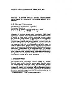
3. Hybrid Optimization Algorithm Based on PSO and FWA The exploitation process focuses on utilizing the existing information to look for better solutions, whereas the exploration process attaches importance to seek the optimal solutions in the entire space. For PSO, under the guidance of their historical best solutions and the current global best solution, the particles can quickly find better solutions, and the excellent exploitation efficiency of algorithm is shown. In FWA, the fireworks can find the global optimal solution in the whole search space by performing explosion and mutation operations while the outstanding exploration capability of FWA is demonstrated. To utilize the advantages of the two algorithms, a hybrid optimization method (PS-FW) based on PSO and FWA is proposed. 3.1. Feasibility Analysis. The formation of a hybrid algorithm is mainly due to the effective combination of the operators of its composition algorithms in a certain way. To clarify the performance enhancement caused by combining the PSO algorithm with fireworks algorithm, we draw Figures 1 and 2 to illustrate the optimization mechanism. As shown in Figure 1, for standard PSO algorithm, the 𝑖th particle moves from point 1 to point 4 under the common influence of velocity inertia, self-cognition, and social information. When the operators of FWA are added, the particle is transformed into firework and performs explosion and mutation operations and eventually reaches the position of firework or sparks, such as point 5 shown in Figure 1. By performing the

4


it

c1 · r1 · (pbestit − xit ) 3

c2 · r2 · (gbestt − xit ) 4

Explosion

Mutation

2 w·

Local optima region

it

5 t+1 xi

pbestit

xit 1

gbestt

Figure 1: Optimization mechanism of adding operators of FWA to PSO algorithm.

gbestt pbestit

2

Explosion

xit Mutation

1

5 xit+1

4 Global optima region

3 it

Figure 2: Optimization mechanism of adding operators of PSO to FWA.

operators of FWA, the particle can explore better solutions in multiple directions and jump out of the local optima region as depicted in Figure 1. Thus we can argue that the operators of FWA improve the global search ability of PSO algorithm. As we know, the searching region is determined by the explosion amplitude and fireworks with poor quality have bigger amplitude, which may lead to an uncomprehensive search without considering the cooperation with other fireworks. When the firework with poor quality generates the explosion sparks and mutation sparks, the new selected location may skip over the global optima region without the attraction from the rest of fireworks and arrive at point 2. By adding the operators of PSO after the 𝑖th firework updates its location, the information of its own historical best location and current global best location is taken into account; then the new solution is found in point 5, which is shown in Figure 2. Therefore, the operators of PSO could strengthen the local search efficiency of FWA. Based on the above analysis, it is concluded that the combination of PSO and FWA is an effective way to form a superior optimization algorithm. 3.2. The Abandonment and Supplement Mechanism. The particles with their memory ability can be quickly converged

to the current optimal solution. However, the aggregation effect of the particle swarm reduces the diversity of the population, which makes the search in the whole feasible space inefficient. In this paper, in order to enhance the balance between exploitation ability and exploration ability of PS-FW, we adopt the abandonment and supplement strategy which includes three main steps. (i) All the particles in the particle swarm 𝑥1 , 𝑥2 , . . . , 𝑥𝑀 are sorted in ascending order. Then the 𝑃num particles with better fitness are retained for the next iteration, and the FWnum (satisfying 𝑃num + FWnum = 𝑀) particles with lower fitness are abandoned. (ii) The 𝑃num excellent individuals denoted as 𝑥𝐹1 , 𝑥𝐹2 , . . . , 𝑥𝐹𝑃num are used to implement the explosion operator, the mutation operator, and the selection operator. (iii) The new individuals obtained by the operators of FWA are added to the original population, to balance the number of particles and to generate the new particle swarm for the next iteration. The abandonment and supplement strategy not only retains the information of the excellent individuals so that they can participate in the subsequent calculation, but also avoids the individuals with poor quality wasting computing resources. However, the problem arises: how to determine 𝑃num ? For this, through analyzing the process of solving the optimization problems, we should enhance the exploration ability of the algorithm and search the optimal solution in the global scope at early stage of iterations, which means the number of particles executing the operators of FWA should be the majority. In the later stage of iteration, we should focus on searching around the current global optimal solution, so the number of excellent individuals retained in the algorithm should be more. Based on the discussion above, the calculation of FWnum in this paper is shown in (9), in which FWnum decreases with iteration process. FWnum = round [(FWmax − FWmin ) ⋅ (

𝐼max − 𝑡 𝑟 ) 𝐼max

(9)

+ FWmin ] , where FWmax and FWmin are the upper and lower bounds of number of abandoned particles, respectively, 𝐼max is the maximum number of iterations, 𝑡 denotes the current number of iterations, round[] indicates that the values in brackets are rounded, and 𝑟 represents a positive integer. 3.3. Modified Explosion Operator 3.3.1. Adaptive Explosion Amplitude. Based on the analysis above, the definition of the explosion amplitude in standard FWA limits the diversity of the explosion sparks generated by the excellent fireworks, thus decreasing the local search ability of algorithm. In the enhanced fireworks algorithm (EFWA) [29], in order to avoid the weakness of the explosion amplitude generation in FWA, a minimal explosion amplitude check mechanism is proposed, which defines the explosion amplitude less than a certain threshold to obtain the same value as the threshold while the threshold is reducing with the iteration process. Suppose that 𝛿 denotes the threshold of


5

explosion amplitude; then the explosion amplitude less than the threshold is defined as (10) in EFWA.

to the fitness. (ii) Update the explosion amplitude of the 𝑖th firework according to the following equation:

̂ ̂ ̂= 𝐴 ̂init − 𝐴 init − 𝐴 final ⋅ √(2𝐼max − 𝑡) 𝑡, 𝐴 𝐼max

󵄨󵄨 󵄨󵄨 󵄨 󵄨 ∑𝐷 𝑘=1 (󵄨󵄨𝑥best,𝑘 − 𝑥𝑗,𝑘 󵄨󵄨) ̂𝑖 = , 𝐴 𝐷

(10)

̂final are the upper and lower bounds of the ̂init and 𝐴 where 𝐴 explosion amplitude, respectively. In this paper, based on the minimal explosion amplitude detection mechanism, the basic explosion amplitude of each firework is calculated according to (3), and the explosion amplitude is adjusted by the following two methods. (1) For the fireworks whose explosion amplitude is greater than the threshold 𝛿, a control factor 𝜆 of the explosion amplitude is added. The control factor makes the explosion sparks generated by the algorithm have larger search scope in the early stage of iterations, which can effectively enhance the exploration ability of the algorithm. In the later stage of iterations, the explosion amplitude is reduced to improve the search efficiency around the current global optimal solution. The adjustment of the explosion amplitude is shown in (11), and the control factor is calculated as shown in (12). ̂𝑖 ⋅ 𝜆, ̂𝑖 = 𝐴 𝐴 𝜆 = 𝜆 min ⋅ (

̂𝑖 > 𝛿, ∀𝐴

(11)

𝜆 max 1/(1+𝑡/𝐼max ) ) , 𝜆 min

(12)

where 𝜆 max and 𝜆 min are the lower and upper bounds of the control factor, respectively. (2) When the explosion amplitude of firework 𝑥𝑖 is less than the threshold, the optimal firework and its neighbor information are used to determine the explosion amplitude in the hybrid algorithm. Since the PS-FW algorithm is based on the framework of PSO, the position of all individuals will approach the current best position, which leads to the fitness of current optimal individual close to its neighbor individuals. That is to say, if the explosion amplitude of a firework is too small, indicating that the firework may be located near the current best location, therefore, by considering the deviation information of all corresponding dimensions between the current best firework and its neighbor firework, a new explosion amplitude of the firework 𝑥𝑖 is generated. The explosion amplitude generation method can adaptively optimize the solving process, which can be interpreted from two aspects. When the algorithm is in the early iteration stage, the position of fireworks is scattered, and the deviation in dimensions between the optimal firework and its neighbor firework is larger, which leads to the larger explosion amplitude and the improved probability of finding the global optimal solution. As the algorithm enters the later iterations, the fireworks gather around the current best location, and the offset of each dimension between the current best firework and its neighbor firework is reduced, which results in the decrement of explosion amplitude and the improvement of the local search ability for PS-FW. There are two main steps to obtain the explosion amplitude. (i) Randomly select a firework 𝑥𝑗 around the current optimal firework according

(13)

where 𝑥best,𝑘 denotes the value of the 𝑘th dimension of current optimal firework. 3.3.2. Modified Explosion Sparks Generation. In FWA, when generating an explosion spark, the offset Δℎ is only calculated once, which results in the same changes for all the selected dimensions and an ineffective search for different directions. In the PS-FW algorithm proposed in this paper, a new explosion sparks generation method is introduced. Firstly, when generating the explosion sparks, the location offset is performed in all the dimensions of the fireworks instead of randomly selecting part of dimensions. Furthermore, for each dimension of the fireworks, the different offsets are calculated according to (14), thereby increasing the diversity of the explosion sparks and the global search capability of the hybrid algorithm. Meanwhile, suppose that 𝑥temp denotes the 𝑖th firework without a location offset and 𝑥+ indicates the 𝑖th firework whose 𝑘th dimension adds a offset; then 𝑥− denotes the 𝑖th firework whose 𝑘th dimension subtracts an offset. As shown in (15), inspired by greedy algorithm, when the fireworks generate their explosion sparks, the hybrid algorithm determines which offset to be selected based on the value of objective function, which can effectively improve the local search capability of the algorithm and accelerate the convergence. ̂ ⋅ Gaussian (0, 1) , Δ̂ℎ𝑘 = 𝐴

(14)

𝑗

𝑥̂𝑖,𝑘 𝑥𝑖,𝑘 + Δ̂ℎ𝑘 , 𝑓 (𝑥+ ) ≤ min (𝑓 (𝑥temp ) , 𝑓 (𝑥− )) { { (15) { { = {𝑥𝑖,𝑘 − Δ̂ℎ𝑘 , 𝑓 (𝑥− ) ≤ min (𝑓 (𝑥temp ) , 𝑓 (𝑥+ )) { { { 𝑓 (𝑥temp ) ≤ min (𝑓 (𝑥+ ) , 𝑓 (𝑥− )) , {𝑥𝑖,𝑘 , 𝑗 where 𝑥̂𝑖,𝑘 and Δ̂ℎ𝑘 are the value and offset of the 𝑘th dimension of the 𝑗th explosion spark for the 𝑖th firework, respectively, Gaussian(0, 1) represents a random number that follows the standard normal distribution, 𝑖 and 𝑗 are integers in the intervals [1, 𝑃num ] and [1, 𝑠𝑖 ], respectively, and min() indicates the minimum values in parentheses. Assume that num𝐸 denotes the total number of explosion sparks generated by all fireworks, 𝑆min and 𝑆max represent the lower and upper bounds for the search scope, and 𝑆min,𝑘 and 𝑆max,𝑘 are corresponding to the bounds of 𝑘th dimension, respectively. Based on the explosion operator introduced in Sections 3.3.1 and 3.3.2, the detailed codes of explosion operator are represented in Algorithm 1.

3.4. Novel Mutation Operator. As the Gaussian mutation operator effectively increases the diversity of feasible solutions, the performance of traditional FWA has been significantly improved. However, the numerical experiments

6


(1) Input: 𝑃num particles sorted in ascending order according to their fitness. (2) Initialize the location of fireworks: 𝑥𝑖 = 𝑥𝐹𝑖 , 𝑖 = 1, 2, . . . , 𝑃num . (3) for 𝑖 = 1 to 𝑃num do (4) Calculate the explosion amplitude 𝐴 𝑖 of 𝑖th firework by using (3). (5) Calculate the number of explosion sparks 𝑠𝑖 of 𝑖th firework by using (4). (6) Update the number of explosion sparks of 𝑖th firework by using (5). ̂𝑖 > 𝛿 do (7) if 𝐴 (8) Update the explosion amplitude of 𝑖th firework by using (11) and (12). (9) else do (10) Randomly select a firework 𝑥𝑗 around the current optimal firework. (11) Update the explosion amplitude of 𝑖th firework by using (13). (12) end if (13) end for (14) Initialize the total number of explosion sparks num𝐸 = 0. (15) for 𝑖 = 1 to 𝑃num do (16) for 𝑗 = 1 to 𝑠𝑖 do 𝑗 (17) Initialize the location of the 𝑗th explosion spark: 𝑥̂𝑖 = 𝑥𝑖 . (18) for 𝑘 = 1 to 𝐷 do (19) Calculate the offset by using (14). (20) Update the value of 𝑘th dimension of 𝑗th explosion spark by using (15). 𝑗 𝑗 (21) if 𝑥̂𝑖,𝑘 > 𝑆max,𝑘 or 𝑥̂𝑖,𝑘 < 𝑆min,𝑘 do 𝑗 (22) Update the 𝑥̂𝑖,𝑘 by using (17). (23) end if (24) end for (25) num𝐸 = num𝐸 + 1 (26) end for (27) end for (28) Output: num𝐸 explosion sparks. Algorithm 1: Generating explosion sparks by the explosion operator of PS-FW.

show that the combined application of Gaussian operator and mapping operator makes the Gaussian sparks mostly concentrated around the zero point, which is the reason why FWA has the fast convergence speed for the problems with their optimal solutions at zero [31]. In order to improve the adaptability of the algorithm for the nonzero optimization problems and maintain the contribution of the mutation operator to the population diversity, a new mutation operator is proposed in the PS-FW. Compared with the standard FWA, there are two main differences in this paper. (i) In PS-FW, we randomly select a certain number of explosion sparks to generate the mutation sparks instead of using the fireworks. Because the explosion sparks have better quality compared to the fireworks based on (15), the mutation sparks generated by the explosion sparks can effectively enrich the diversity of the population and have better global search ability. (ii) In this paper, the Gaussian random number is no longer used in mutation operator and the interaction mechanism of particles in PSO is used for reference to design the mutation operator. The mutation sparks generated by our mutation operator can not only maintain the better information of the explosion sparks, but also have a proper movement towards the current best location, which leads to promoting the convergence of hybrid algorithm. The proposed mutation operator is shown as follows. 𝑥̃𝑖,𝑘 = 𝜇1 ⋅ (𝑥̂best,𝑘 − 𝑥̂𝑗,𝑘 ) + 𝜇2 ⋅ 𝑥̂𝑗,𝑘 ,

(16)

where 𝑥̃𝑖,𝑘 and 𝑥̂𝑗,𝑘 indicate the value of 𝑘th dimension of 𝑖th mutation spark and 𝑗th explosion spark, respectively, 𝑥̂best,𝑘 is the current optimal explosion spark, 𝜇1 and 𝜇2 are the random number in [0, 1], and 𝑗 denotes the random integer of the interval [1, num𝐸 ], 𝑖 = 1, 2, . . . , num𝑀, where num𝑀 indicates the total number of mutation sparks. The detailed codes of mutation operator are represented in Algorithm 2. 3.5. Main Process of PS-FW. In PS-FW, the algorithm consists of two main stages, which are initialization stage and iterations stage. In the initialization phase, we need to initialize the position and velocity of the particle swarm, as well as to initialize the control parameters. In the iterative phase, the PS-FW algorithm inherits all the parameters and operators of the PSO algorithm, and all particles are used as the main carrier for storing feasible solutions. Firstly, in each iteration, the particles update their speed and position according to the operators of the PSO algorithm and then perform the abandonment and supplement operation. Besides, in the process of generating the supplement particles by using the operators of FWA, we first generate num𝐸 explosion sparks according to the excellent 𝑃num particles and the modified explosion operator; then the fitness of the explosion sparks is given. Secondly, the num𝑀 mutation sparks are generated by the explosion sparks and the novel mutation operator. Finally, the FWnum supplement individuals are selected by the


7

4. Problems, Experiments, and Discussion (1) Input: num𝐸 explosion sparks and best explosion spark 𝑥̂best (2) for 𝑖 = 1 to num𝑀 do (3) Generate a random integer 𝑗 in the interval [1, num𝐸 ]. (4) Initialize the location of the 𝑖th mutation spark: 𝑥̃𝑖 = 𝑥̂𝑗 . (5) Calculate the number of dimensions to perform the mutation: 𝑧̃𝑖 = 𝐷 ⋅ rand(). (6) Randomly select 𝑧̃𝑖 dimensions of 𝑥̃𝑖 . (7) for each dimension 𝑥̃𝑖,𝑘 ∈ pre-selected 𝑧̃𝑖 dimensions of 𝑥̃𝑖 do (8) Calculate the value of 𝑥̃𝑖,𝑘 by using (16). (9) if 𝑥̃𝑖,𝑘 > 𝑆max,𝑘 or 𝑥̃𝑖,𝑘 < 𝑆min,𝑘 do (10) Update the value of 𝑥̃𝑖,𝑘 by using (17). (11) end if (12) end for (13) end for (14) Output: num𝑀 mutation sparks. Algorithm 2: Generating mutation sparks by the mutation operator of PS-FW.

combination of elite strategy and roulette strategy. When each iteration is completed, it is judged whether the termination condition is satisfied. If the stopping criterion is matched, the iteration will be stopped and the best solutions are output. Otherwise, the iteration phase will be repeated. In the procedures above, there are two points to be noted. (i) In the implementation process of the hybrid algorithm, it is necessary to detect whether the position of individuals is within the feasible scope while the individuals consist of particles, fireworks, explosion sparks, and mutation sparks. As shown in (17), if the position of individuals exceeds the feasible scope, it is adjusted by using the mapping criteria in the EFWA algorithm [29]. 𝑌𝑖,𝑘 = 𝑆min,𝑘 + 𝑒 ⋅ (𝑆max,𝑘 − 𝑆min,𝑘 ) ∀𝑌𝑖,𝑘 > 𝑆max,𝑘 or 𝑌𝑖,𝑘 < 𝑆min,𝑘 ,

(17)

where 𝑌𝑖,𝑘 indicates the value of the 𝑘th dimension of the individual and 𝑒 is a random number in [0, 1]. (ii) The selection strategy of FWA based on the density of feasible solutions is abandoned in the PS-FW algorithm. Although it is possible to maintain the diversity of the population by selecting the location which has fewer individuals around with a larger probability, relatively more time is wasted by calculating the spatial distance between the individuals and the efficiency of the algorithm is reduced. Therefore, a selection strategy based on fitness is applied in PS-FW, which means the elite strategy is used to retain the best individual directly into the next iteration and the remaining FWnum − 1 locations are selected by the roulette criterion according to the fitness. According to the description above, the main codes of the PS-FW algorithm are given in Algorithm 3.

4.1. Test Problems. In order to evaluate the efficacy and accuracy of the proposed algorithm, the performance of PS-FW is tested by the 22 high-dimensional benchmark functions. The test problems which consist of multimodal functions and unimodal functions are listed in Table 1, and the corresponding optimal solutions and search scope are presented in Table 1. Compared with solving unimodal problems, it is difficult to find the global optimum of multimodal problems because the local optima will induce the optimization algorithms’ fall into their surroundings. Therefore, if the algorithm can efficiently find the optimal solutions of multimodal functions, it can be proved that the algorithm is an excellent optimization algorithm. 4.2. Comparison of PS-FW with PSO and FWA. In this section, we compare the performance of the PS-FW with the PSO and FWA based on the 22 benchmark functions. In order to explore global optimization capability of the three algorithms on solving the high-dimensional optimization problem, three experiments with different dimensions are carried out. The dimensions of experiments are set to 𝐷 = 30, 𝐷 = 60, and 𝐷 = 100, respectively, and each algorithm is used to solve all the benchmark functions 20 times independently. In order to make a fair comparison, the general control parameters of algorithms such as the maximum number of iterations (𝐼max ) and the population size (𝑀) are set to be of the same value. 𝐼max is set to 1000 and 𝑀 is set to 50 for each function. Besides, the algorithms used in the experiment are coded by MATLAB 14.0, and the experiment platform is a personal computer with Core i5, 2.02 GHz CPU, 4 G memory, and Windows 7. For the purpose of eliminating the impact on performance caused by the difference in parameter settings, the main control parameters of PS-FW algorithm are consistent with those of PSO and FWA, and the other detailed control parameters are shown in Table 2. For all the benchmark functions, the mean and standard deviation of best solutions obtained by PS-FW and other algorithms in 20 independent runs are recorded, and the optimization results are shown in Tables 3–5. Meanwhile, the ranks are also presented in tables, and the three algorithms are ranked mainly based on the mean of best solutions. In addition, the average convergence speed of the proposed PSFW is compared with other algorithms for functions 𝑓12 , 𝑓13 , and 𝑓20 ; therefore the convergence curves are shown in Figure 3. According to the ranks shown in Tables 3–5, the average values of best solutions for the proposed PS-FW outperform those of the other algorithms. Besides, the performance of PS-FW over standard deviation of best solutions is also better than the rest of the algorithms. For 22 problems with 𝐷 = 30, the PS-FW can obtain the global optimum of 𝑓2 , 𝑓3 , 𝑓4 , 𝑓5 , 𝑓6 , 𝑓8 , 𝑓12 , 𝑓15 , 𝑓17 , 𝑓18 , 𝑓20 , and 𝑓21 , which shows excellent ability for solving optimization problems. As the dimensions of problems increase, the hybrid algorithm maintains outstanding performance and obtains the optimal solutions of the 10 functions, except for functions 𝑓3 and 𝑓6 , compared with results in Table 3. When the dimensions of

8


(1) Input: Objective function 𝑓(𝑥) and constraints. (2) Initialization ̂ 𝑀𝑒 , 𝜀, 𝛿, 𝑎, 𝑏, 𝑟, num𝑀 , 𝐼max , FWmax , FWmin , 𝜆 min , 𝜆 max (3) Parameters initialization: assign values to 𝑀, 𝑤max , 𝑤min , 𝑐1 , 𝑐2 , 𝐴, (4) Population initialization: generate the random values for 𝑥𝑖 and V𝑖 of each particle in the feasible domain, calculate the 𝑔𝑏𝑒𝑠𝑡 of initial population. (5) Set 𝑝𝑏𝑒𝑠𝑡𝑖 = 𝑥𝑖 , (𝑖 = 1, 2, . . . , 𝑀) and 𝑡 = 0. (6) Iterations (7) while 𝑡 ≤ 𝐼max (8) 𝑡 = 𝑡 + 1 (9) for 𝑖 = 1 to 𝑀 (10) for 𝑗 = 1 to 𝐷 (11) Update the velocity of particle 𝑥𝑖 by using (1). (12) Update the position of particle 𝑥𝑖 by using (2). (13) if 𝑥𝑖,𝑘 > 𝑆max,𝑘 or 𝑥𝑖,𝑘 < 𝑆min,𝑘 (14) Update the value of 𝑥𝑖,𝑘 by using (17). (15) end if (16) end for (17) end for (18) Calculate FWnum by using the (9). (19) Sort the particle population in ascending order and select the 𝑃num particles with better fitness. (20) Generate num𝐸 explosion sparks by using Algorithm 1. (21) Calculate the fitness of explosion sparks and storage the best explosion spark 𝑥̂best . (22) Generate num𝑀 mutation sparks by using Algorithm 2. (23) Select the FWnum individuals from the explosion sparks and mutation sparks by using the selection strategy. (24) Combine the 𝑃num particles with FWnum individuals to generate the new population. (25) Calculate 𝑔𝑏𝑒𝑠𝑡 and 𝑝𝑏𝑒𝑠𝑡𝑖 of new population. (26) end while (27) Output: 𝑔𝑏𝑒𝑠𝑡 = (𝑔𝑏𝑒𝑠𝑡1 , 𝑔𝑏𝑒𝑠𝑡2 , . . . , 𝑔𝑏𝑒𝑠𝑡𝐷 ) Algorithm 3: The main codes of PS-FW algorithm.

problems are 60 and 100, PS-FW can get the global optimum of functions 𝑓3 and 𝑓6 , but not each run can succeed. This is because functions 𝑓3 and 𝑓6 are multimodal problems and the number of local optima increases rapidly as the dimensions of the problems increase, which adds the difficulty of avoiding trapping in the local optima. In addition, according to the ranks and values shown in Tables 3–5, the PS-FW can get the highest rank for all the functions. It is also needed to point out that the PS-FW obtains more stable solutions than PSO and FWA for all problems with the increasing of dimensionality. The convergence speed of the three algorithms can be seen in Figure 3, and the descend rate of average best solutions of PS-FW is obviously higher than the other two algorithms. This is because the advantages of PSO and FWA are combined into the PS-FW so that the hybrid algorithm enhances its global and local search ability. Therefore, PS-FW is efficient and robust in dealing with the high-dimensional benchmark functions. From the above analysis, it is possible to show that the PS-FW algorithm performs well in solving the functions in Table 1. However, because the optimums of these functions are mostly at the origin, we need to further explore the performance of PS-FW algorithm on the nonzero problems. Then the experiment of nonzero problems is carried out to prove the comprehensive performance of PS-FW. In this experiment, the optimums of test functions derived from Table 1 are shifted and the specific values are displayed in

Table 6. In addition, in order to achieve a fair comparison between the experiments, the parameters settings of three algorithms are consistent with Table 2 and the dimension is set to 𝐷 = 30. The optimization results of three algorithms are shown in Table 7 and the convergence curves of three algorithms over functions 𝑓12 , 𝑓13 , and 𝑓20 are displayed in Figure 4. From Table 7, we can know that the PS-FW algorithm keeps high performance and can obtain the optimal solutions of 11 functions in Table 6. Besides, the PS-FW achieves the best rank of three algorithms for all the functions with shift optimums, which present the powerful solving ability over optimization problems with nonzero optimums. By comparing Table 7 with Table 3, it is known that fireworks algorithm is relatively weak in searching for nonzero optimums. However, the PS-FW algorithm that derives from the fireworks algorithm and covers operators of PSO shows better performance, which demonstrates the correctness of the combination of the two algorithms. In addition, the result of PS-FW over function 16 is worse than the previous experiment. This is because 𝑓16 is a multimodal function and the slight deviations from the optimums can cause the significant increase in the value of the objective function. By observing the convergence curves in Figure 4, we can state that the convergence speed of the PS-FW also remains fast. In order to determine whether the convergence performance of PS-FW algorithm is superior to the other two algorithms


9

Table 1: The 22 high-dimensional benchmark functions. Name

Search space

Optimum

[−100, 100]𝐷

0

[−600, 600]𝐷

0

[−5, 10]𝐷

0

[−5.12, 5.12]𝐷

0

[−5, 10]𝐷

0

[−30, 30]𝐷

0

[−65536, 65536]𝐷

0

𝑓8 (𝑥) = ∑𝑖𝑥4 + rand

[−1.28, 1.28]𝐷

0

󵄨 󵄨 𝑓9 (𝑥) = max 󵄨󵄨󵄨𝑥𝑖 󵄨󵄨󵄨 1≤𝑖≤𝐷

[−100, 100]𝐷

0

[−100, 100]𝐷

0

[−500, 500]𝑑

−418.9829𝐷

[−10, 10]𝐷

0

[−10, 10]𝐷

0

[−1, 1]𝐷

0

[−10, 10]𝐷

0

[−5, 10]𝐷

0

[−𝐷, 𝐷]𝐷

0

[−0.5, 0.5]𝐷

0

[−100, 100]𝐷

0

Function 𝐷

Sphere

𝑓1 (𝑥) = ∑𝑥𝑖2 𝑖=1

𝑥 1 𝐷 2 𝐷 ∑𝑥 − ∏ cos ( 𝑖 ) + 1 √𝑖 4000 𝑖=1 𝑖 𝑖=1

Griewank

𝑓2 (𝑥) =

Rosenbrock

𝑓3 (𝑥) = ∑ [100 (𝑥𝑖+1 − 𝑥𝑖2 ) + (𝑥𝑖 − 1) ]

𝐷−1

2

2

𝑖=1

𝐷

Rastrigin

𝑓4 (𝑥) = 10𝐷 + ∑ [𝑥𝑖2 − 10 cos (2𝜋𝑥𝑖 )] 𝑖=1

𝐷

𝑓5 (𝑥) = ∑𝑦𝑖2 − 10 cos(2𝜋𝑦𝑖 ) + 10 𝑖=1

Noncontinuous Rastrigin

󵄨󵄨 󵄨󵄨 󵄨󵄨𝑥𝑖 󵄨󵄨 < 0.5

{ { {𝑥𝑖 𝑦𝑖 = { { { round (2𝑥𝑖 ) { 2

󵄨󵄨 󵄨󵄨 󵄨󵄨𝑥𝑖 󵄨󵄨 ≥ 0.5

Ackley

𝑓6 (𝑥) = −20 exp (−0.2√

Rotated Hyper-Ellipsoid

𝑓7 (𝑥) = ∑ ∑𝑥𝑗2

𝐷

1 𝐷 2 1 𝐷 ∑𝑥𝑖 ) − exp ( ∑ cos (2𝜋𝑥𝑖 )) + 20 + 𝑒 𝐷 𝑖=1 𝐷 𝑖=1

𝑖

𝑖=1 𝑗=1 𝐷

Noisy Quadric

𝑖=1

Schwefel’s problem 2.21 Schwefel’s problem 2.22

𝐷

𝐷

𝑖=1

𝑖=1

󵄨 󵄨 󵄨 󵄨 𝑓10 (𝑥) = ∑ 󵄨󵄨󵄨𝑥𝑖 󵄨󵄨󵄨 + ∏ 󵄨󵄨󵄨𝑥𝑖 󵄨󵄨󵄨 𝐷

Schwefel’s problem 2.26

󵄨 󵄨 𝑓11 (𝑥) = ∑ − 𝑥𝑖 sin (√󵄨󵄨󵄨𝑥𝑖 󵄨󵄨󵄨) 𝑖=1 𝐷

Step

𝑓12 (𝑥) = ∑ ([𝑥𝑖 + 0.5])

2

𝑖=1

𝐷−1

2

𝑓13 (𝑥) = sin2 (𝜋𝑦1 ) + ∑ (𝑦𝑖 − 1) [1 + 10 sin2 (𝜋𝑦𝑖 + 1)] Levy

2

𝑖=1

+ (𝑦𝐷 − 1) [1 + sin2 (2𝜋𝑦𝐷 )] 𝑥 −1 𝑦𝑖 = 1 + 𝑖 4 𝐷

Powell Sum

󵄨 󵄨𝑖+1 𝑓14 (𝑥) = ∑ 󵄨󵄨󵄨𝑥𝑖 󵄨󵄨󵄨 𝑖=1 𝐷

Sum squares

𝑓15 (𝑥) = ∑𝑖𝑥𝑖2 𝑖=1

Zakharov

𝐷

𝐷

𝑖=1

𝑖=1

𝐷

4

𝑖=1

2

𝐷

Mishra 7

2

𝑓16 (𝑥) = ∑𝑥𝑖2 + (∑0.5𝑖𝑥𝑖 ) + (∑0.5𝑖𝑥𝑖 ) 𝑓17 (𝑥) = (∏𝑥𝑖 − 𝐷!) 𝑖=1

Weierstrass

𝐷

𝑘max

𝑘max

𝑖=1

𝑘=0

𝑘=0

𝑓18 (𝑥) = ∑ [ ∑ (𝑎𝑘 cos (2𝜋𝑏𝑘 (𝑥𝑖 + 0.5))) − 𝐷 ∑ 𝑎𝑘 cos (𝜋𝑏𝑘 )] 𝑎 = 0.5, 𝑏 = 3, 𝑘max = 20 𝐷

Bent-Cigar

𝑓19 (𝑥) = 𝑥12 + 106 ∑𝑥𝑖2 𝑖=1

10

Computational Intelligence and Neuroscience Table 1: Continued.

Name

Function 𝐷

2

2

𝑓20 (𝑥) = 1+ ∑8 sin2 [7 (𝑥𝑖 − 0.9) ]+6 sin2 [14 (𝑥𝑖 − 0.9) ]+(𝑥 − 0.9)2

Trigonometric 2

Search space

Optimum

[−500, 500]𝐷

1

[−10, 10]𝐷

0

[−10, 10]𝐷

0

𝑖=1

𝐷 󵄨 󵄨 𝑓21 (𝑥) = ∑ 󵄨󵄨󵄨󵄨𝑥𝑖5 − 3𝑥𝑖4 + 4𝑥𝑖3 + 2𝑥𝑖2 − 10𝑥𝑖 − 4󵄨󵄨󵄨󵄨

Quintic

𝑖=1

𝐷

Mishra 11

106

10−14 10−24 0

200

400 600 Iteration

800

10−4 10−14 10−24 10−34

1000

107

0

(a) 𝑓12 with 𝐷 = 30

200

400 600 Iteration

800

10−13 10−23 0

Average best fitness

5

104 10

101 10

0

0

200

400 600 Iteration

800

10−14 10−24 10−34

1000

400 600 Iteration

800

1000

10

103 102 101 0

200

400 600 Iteration

PSO FWA PS-FW

PSO FWA PS-FW (g) 𝑓20 with 𝐷 = 30

(h) 𝑓20 with 𝐷 = 60

200

400 600 Iteration

800

1000

(f) 𝑓13 with 𝐷 = 100

104

100

0

PSO FWA PS-FW

(e) 𝑓13 with 𝐷 = 60

106

2

200


(d) 𝑓13 with 𝐷 = 30

5

800 1000

10−4

PSO FWA PS-FW

106

400 600 Iteration

(c) 𝑓12 with 𝐷 = 100

10−3

10−33

1000

200

106

PSO FWA PS-FW

10

0

PSO FWA PS-FW



10−23



10−13

0

10−23 10−33

800 1000

107

10−3

3

400 600 Iteration

10−13

(b) 𝑓12 with 𝐷 = 60

107

10

200

10−3

PSO FWA PS-FW

PSO FWA PS-FW

10−33

]


10−4

10−34

2

]

106 Average best fitness


1/𝐷

𝐷

1 󵄨 󵄨 󵄨 󵄨 𝑓22 (𝑥) = [ ∑ 󵄨󵄨󵄨𝑥𝑖 󵄨󵄨󵄨 + (∏ 󵄨󵄨󵄨𝑥𝑖 󵄨󵄨󵄨) 𝐷 𝑖=1 𝑖=1 [

800

1000

107 106 105 104 103 102 101 100

0

200

400 600 Iteration

PSO FWA PS-FW (i) 𝑓20 with 𝐷 = 100

Figure 3: Convergence curves of PSO, FWA, and PS-FW for functions 𝑓12 , 𝑓13 , and 𝑓20 .

800

1000


−13

10−23 10

−33

0

200

400 600 Iteration

800

1000


10−3 10

106

107 Average best fitness


107

11

10−3 10

−13

10−23 10

−33

0

PSO FWA PS-FW (a) 𝑓12 with 𝐷 = 30

200

400 600 Iteration

800

1000

105 104 103 102 101 100

0

200

400 600 Iteration

800

1000

PSO FWA PS-FW

PSO FWA PS-FW (b) 𝑓13 with 𝐷 = 30

(c) 𝑓20 with 𝐷 = 30

Figure 4: Convergence curves of PSO, FWA, and PS-FW for functions 𝑓12 , 𝑓13 , and 𝑓20 .

Table 2: The parameter setting of the algorithms. Algorithm PSO FWA

PS-FW

Parameter settings 𝑤 − 𝑤min , 𝑤max = 0.95, 𝑤(𝑡) = 𝑤max − 𝑡 max 𝐼max 𝑤min = 0.4, 𝑐1 = 𝑐2 = 1.45 ̂ = 40, 𝑀𝑒 = 50, 𝑎 = 0.04, 𝑏 = 0.8, 𝐴 num𝑀 = 30, 𝜀 = 1𝐸 − 100 𝑤 − 𝑤min 𝑤(𝑡) = 𝑤max − 𝑡 max , 𝑤max = 0.95, 𝐼max ̂ = 40, 𝑤min = 0.4, 𝑐1 = 𝑐2 = 1.45, 𝐴 𝑀𝑒 = 50, 𝑎 = 0.04, 𝑏 = 0.8, num𝑀 = 30, 𝜀 = 1𝐸 − 100, 𝛿 = 1𝐸 − 6, 𝜆 min = 1𝐸 − 25, 𝜆 max = 1, FWmax = 30, FWmin = 20, 𝑟 = 2

more clearly, we compute the number of successful runs (success rate) and the average number of iterations in successful runs for each function in Table 6. The optimal solutions obtained by different algorithms are various, so we define the convergence criterion for each function. The convergence criterion can be introduced as that if the best solutions 𝑓find found by each of algorithms are satisfying (18) in a run [39], the run is considered to be successful, and the minimum number of iterations satisfying the convergence criterion is counted to calculate the average number of iterations. 󵄨󵄨󵄨𝑓 − 𝑓 󵄨󵄨󵄨 < 𝜏, (18) 󵄨󵄨 find opti 󵄨󵄨 where 𝑓opti is the optimum of function and 𝜏 denotes the error of algorithm. Suppose that ST denotes the number of successful runs, AI indicates the average number of iterations in successful runs, and 𝑈 denotes the iterations number when there are no successful runs after 20 runs and its value is set to greater than 𝐼max ; then Table 8 is shown as follows. According to the statistical results and ranks presented in Table 8, the success rate and the average iterations number of PS-FW in 20 runs are both superior to other algorithms. For all the benchmark functions in Table 6, the proposed PS-FW can satisfy the convergence criterion for all the 20

runs, whereas the other algorithms can only converge to the criterion for several functions. In addition, the PS-FW obtains the highest ranks for the average number of iterations in successful runs and can converge to the criterion by a relatively small number of iterations. In summary, the PSFW outperforms the other algorithms in terms of stability and convergence speed and is an efficacious algorithm for optimization problems whose optimums are at origin or are shifted. 4.3. Comparison of PS-FW with PSO Variants. In this section, we compare the performance of the proposed PS-FW with several existing variants of PSO which are introduced in a published paper. The comparison is based on the 12 benchmark functions introduced in the paper of Nickabadi et al. [22] and the orders of functions are consistent with that in this paper. In order to make a fair comparison, the run times and maximum iterations of PS-FW are set to 30 and 200,000, respectively, and the other parameters are set to be the same as those in Section 4.2. The dimension of test problems is set to 𝐷 = 30, and the mean and standard deviation of best solutions obtained by algorithms are calculated. The contrast results are presented in Table 9, and the rank of each algorithm is counted and shown. According to the results of Table 9, the PS-FW outperforms the other six PSO variants on both the average values and standard deviation of best solutions after 200,000 iterations. Among the 12 benchmark functions, the PS-FW can obtain the optimum of 10 functions, which manifests the highly powerful ability to find the global optimal solution. In addition, the PS-FW acquires the highest rank over almost all the test problems except the function 𝑓11 , which indicates the PS-FW has significant improvement than other algorithms. Besides the analysis of numerical results obtained by PS-FW and other algorithms, we applied the nonparametric statistical tests to prove the superiority of the PS-FW. The Friedman test and Bonferroni-Dunn test are adopted to compare the performance of PS-FW with the other algorithms. The Friedman test is a multiple comparison test, to detect the significant differences among algorithms based on the

12


Table 3: Comparison of the optimization results obtained by PS-FW, PSO, and FWA with 𝐷 = 30 for functions 𝑓1 to 𝑓22 (the best ranks are marked in bold). 𝑓

𝐷

𝑓1

30

𝑓2

30

𝑓3

30

𝑓4

30

𝑓5

30

𝑓6

30

𝑓7

30

𝑓8

30

𝑓9

30

𝑓10

30

𝑓11

30

𝑓12

30

𝑓13

30

𝑓14

30

𝑓15

30

𝑓16

30

Mean Std Rank Mean Std Rank Mean Std Rank Mean Std Rank Mean Std Rank Mean Std Rank Mean Std Rank Mean Std Rank Mean Std Rank Mean Std Rank Mean Std Rank Mean Std Rank Mean Std Rank Mean Std Rank Mean Std Rank Mean Std Rank

PSO 8.8371𝐸 + 01 4.3475𝐸 + 01 3 7.1542𝐸 − 02 1.2385𝐸 − 01 2 5.5766𝐸 + 02 7.4828𝐸 + 02 3 6.6547𝐸 + 01 3.6430𝐸 + 01 2 6.5810𝐸 + 01 4.0117𝐸 + 01 2 0 0 1 1.4156𝐸 + 04 1.0006𝐸 + 04 3 1.0419𝐸 − 03 1.0584𝐸 − 03 3 6.3165𝐸 − 01 6.0679𝐸 − 01 3 1.5661𝐸 + 01 5.0924𝐸 + 00 3 −7.2662𝐸 + 03 6.7867𝐸 + 02 3 6.9734𝐸 − 01 2.8586𝐸 − 01 3 1.7831𝐸 + 01 8.6204𝐸 + 00 3 6.6576𝐸 − 08 5.4575𝐸 − 08 3 0 0 1 2.8937𝐸 + 02 1.5937𝐸 + 02 3

FWA 1.3360𝐸 − 151 5.8057𝐸 − 151 2 0 0 1 2.6882𝐸 + 01 8.3997𝐸 − 01 2 0 0 1 0 0 1 0 0 1 7.6585𝐸 − 83 3.3383𝐸 − 82 2 9.6596𝐸 − 304 0 2 7.4698𝐸 − 54 2.3638𝐸 − 53 2 3.2521𝐸 − 78 1.1460𝐸 − 77 2 −1.0511𝐸 + 04 1.9893𝐸 + 02 2 6.6542𝐸 − 01 5.0080𝐸 − 01 2 6.5460𝐸 + 00 8.6700𝐸 − 01 2 4.5613𝐸 − 191 0 2 0 0 1 1.5997𝐸 − 45 3.5711𝐸 − 45 2

PS-FW 5.8928𝐸 − 264 0 1 0 0 1 0 0 1 0 0 1 0 0 1 0 0 1 4.5128𝐸 − 122 1.8821𝐸 − 121 1 0 0 1 3.1588𝐸 − 97 1.2719𝐸 − 96 1 1.8666𝐸 − 137 8.0013𝐸 − 137 1 −1.2483𝐸 + 04 1.2661𝐸 + 02 1 0 0 1 1.4998𝐸 − 32 0 1 2.1563𝐸 − 291 0 1 0 0 1 1.5471𝐸 − 111 6.0668𝐸 − 111 1


13 Table 3: Continued.

𝑓

𝐷

𝑓17

30

𝑓18

30

𝑓19

30

𝑓20

30

𝑓21

30

𝑓22

30

Mean Std Rank Mean Std Rank Mean Std Rank Mean Std Rank Mean Std Rank Mean Std Rank

Average rank Overall rank

PSO 0 0 1 1.5069𝐸 + 01 4.0495𝐸 + 00 2 2.8450𝐸 + 07 1.2385𝐸 + 08 3 3.8005𝐸 + 02 8.5739𝐸 + 01 3 4.5577𝐸 + 01 2.3091𝐸 + 01 3 7.0166𝐸 − 01 5.9846𝐸 − 01 3 2.5455 3

sets of data [40]. The algorithms are ranked in Friedman test, which means the algorithm with the best performance is ranked minimum, the worst gets the maximum rank, and so on. In this section, the mean and standard deviation of best solutions based on Table 9 are conducted with the Friedman test; therefore the results are given in Table 10. Through observing the results of Friedman test in Table 10, all the 𝑝 value are lower than the level of significance considered 𝛼 = 0.01, which indicates that the significant differences among the seven algorithms do exist. According to the ranks obtained by the Friedman test in Table 10, the PS-FW has the best performance on the mean and standard deviation of best solutions followed by ALWPSO, CLPSO, and the other four algorithms. Therefore, we can conclude that the accuracy of solutions obtained by PS-FW is better than other algorithms. However, the Friedman test can only detect whether there are significant differences among all the algorithms, but is unable to conduct the proper comparisons between PS-FW and each of the other algorithms. Hence the Bonferroni-Dunn test is executed to check the superiority of PS-FW. The Bonferroni-Dunn test can be very intuitive to detect the significant difference between the two or more algorithms. For Bonferroni-Dunn test, the judgment condition for the existence of significant difference between the two algorithms is that their mean ranks differ by at least the critical difference (CD), and the equation of calculating the critical difference is as follows [41]: CD𝛼 = 𝑞𝛼 √

𝑁𝑖 (𝑁𝑖 + 1) , 6𝑁𝑓

(19)

FWA 9.8737𝐸 + 44 4.3038𝐸 + 45 2 0 0 1 1.0123𝐸 − 145 3.1288𝐸 − 145 2 4.2079𝐸 + 01 4.6125𝐸 + 00 2 1.71130𝐸 + 01 2.1499𝐸 + 00 2 1.1989𝐸 − 149 5.2258𝐸 − 149 2 1.7273 2

PS-FW 0 0 1 0 0 1 1.8302𝐸 − 252 0 1 1 0 1 0 0 1 3.5102𝐸 − 292 0 1 1 1

where 𝑁𝑖 and 𝑁𝑓 are the number of algorithms and benchmark functions and the critical values 𝑞𝛼 at the probability level 𝑎 are presented as follows: 𝑞0.05 = 2.77, 𝑞0.1 = 2.54.

(20)

By utilizing (19) and (20), the critical difference is shown as follows: CD0.05 = 2.44, CD0.1 = 2.24.

(21)

Here we carry out the Bonferroni-Dunn test for the mean of best solutions, success rate, and average number of iterations of successful runs on the basis of the ranks obtained by the Friedman test. In order to provide a more intuitive display of the results obtained by Bonferroni-Dunn test, we illustrate the critical differences among the seven algorithms in Figure 5. For the purpose of comparing the algorithms clearly, a horizontal line which indicates the threshold for the best performing algorithm (the one with pink color) is drawn in the graphs. In addition, another two lines which represent each level of significance considered in the paper are also drawn, and their heights are equal to the sum of minimum rank and the corresponding CD. Then if the bars exceed the lines of significant level, the corresponding algorithms are proved to have worse performance than the best performing algorithm. By observing the results of Bonferroni-Dunn test in Figure 5(a), the bar of the PS-FW has the lowest height among all the algorithms, and the heights of bars corresponding to the

14



𝐷

𝑓1

60

𝑓2

60

𝑓3

60

𝑓4

60

𝑓5

60

𝑓6

60

𝑓7

60

𝑓8

60

𝑓9

60

𝑓10

60

𝑓11

60

𝑓12

60

𝑓13

60

𝑓14

60

𝑓15

60

𝑓16

60

Mean Std Rank Mean Std Rank Mean Std Rank Mean Std Rank Mean Std Rank Mean Std Rank Mean Std Rank Mean Std Rank Mean Std Rank Mean Std Rank Mean Std Rank Mean Std Rank Mean Std Rank Mean Std Rank Mean Std Rank Mean Std Rank

PSO 4.1677𝐸 + 03 4.4284𝐸 + 03 3 3.2482𝐸 + 00 9.6094𝐸 − 01 2 7.1638𝐸 + 04 5.5811𝐸 + 04 3 3.2219𝐸 + 02 4.1863𝐸 + 01 2 3.7498𝐸 + 02 5.3191𝐸 + 01 2 1.3162𝐸 + 01 1.1773𝐸 + 00 3 3.2017𝐸 + 04 1.4529𝐸 + 04 3 1.1343𝐸 + 00 3.2234𝐸 + 00 3 2.6902𝐸 + 01 5.4555𝐸 + 00 3 5.5140𝐸 + 01 2.1038𝐸 + 01 3 −1.1892𝐸 + 04 1.1022𝐸 + 03 3 3.4856𝐸 + 01 5.9316𝐸 + 01 3 6.2329𝐸 + 01 2.0956𝐸 + 01 3 2.2365𝐸 − 07 2.3968𝐸 − 07 3 0 0 1 8.0994𝐸 + 02 3.0726𝐸 + 02 3

FWA 2.1235𝐸 − 146 6.3705𝐸 − 146 2 0 0 1 4.5073𝐸 + 01 1.8390𝐸 + 01 2 0 0 1 0 0 1 0 0 1 4.9633𝐸 − 68 1.48899𝐸 − 67 2 1.2096𝐸 − 288 0 2 4.4049𝐸 − 51 1.3214𝐸 − 50 2 1.35612𝐸 − 73 4.06287𝐸 − 73 2 −1.8005𝐸 + 04 1.4727𝐸 + 03 2 1.9695𝐸 + 00 7.7525𝐸 − 01 2 1.5355𝐸 + 01 5.4415𝐸 + 00 2 1.6432𝐸 − 187 0 2 0 0 1 1.7189𝐸 − 38 5.15482𝐸 − 38 2

PS-FW 2.4481𝐸 − 248 0 1 0 0 1 9.2568𝐸 − 30 1.9330𝐸 − 29 1 0 0 1 0 0 1 7.1054𝐸 − 16 1.4211𝐸 − 15 2 1.2294𝐸 − 93 4.9341𝐸 − 93 1 0 0 1 1.5914𝐸 − 92 4.8189𝐸 − 92 1 3.9617𝐸 − 130 1.7268𝐸 − 129 1 −2.4998𝐸 + 04 1.7201𝐸 + 02 1 0 0 1 1.4998𝐸 − 32 0 1 1.5707𝐸 − 278 0 1 0 0 1 6.8924𝐸 − 104 2.9641𝐸 − 103 1



𝑓19

60

𝑓20

60

𝑓21

60

𝑓22

60

8

6

6

Ranks

8

4

4

PS-FW

AIWPSO

CLPSO

Frankenstein

0 FIPS

0 CPSO

2

stdPso

2

PS-FW

Ranks


Algorithms Rank 95% sig. level

90% sig. level Best rank (a) Mean

AIWPSO

60

Frankenstein

𝑓18

PS-FW 0 0 1 0 0 1 4.5120𝐸 − 251 0 1 1 0 1 0 0 1 1.3216𝐸 − 280 0 1 1.0455 1

FIPS

60

FWA 2.4945𝐸 + 145 5.7208𝐸 + 145 2 0 0 1 6.6011𝐸 − 137 1.9631𝐸 − 136 2 1.4665𝐸 + 02 2.8947𝐸 + 01 2 4.8085𝐸 + 01 7.7355𝐸 + 00 2 1.5711𝐸 − 142 4.7133𝐸 − 142 2 1.7273 2

CLPSO

𝑓17

PSO 0 0 1 3.9564𝐸 + 01 5.3138𝐸 + 00 2 5.7753𝐸 + 08 2.7159𝐸 + 08 3 5.3645𝐸 + 03 6.2256𝐸 + 03 3 1.9709𝐸 + 02 2.8605𝐸 + 01 3 1.5314𝐸 + 00 5.9245𝐸 − 01 3 2.6364 3

Mean Std Rank Mean Std Rank Mean Std Rank Mean Std Rank Mean Std Rank Mean Std Rank

CPSO

𝐷

stdPso

𝑓

Algorithms Rank 95% sig. level

90% sig. level Best rank

(b) Standard deviation

Figure 5: The bar chart of Bonferroni-Dunn test for PS-FW and other PSO variants over mean and standard deviation of best solutions based on Table 10.

stdPSO, CPSO, FIPS, and Frankenstein exceed the lines of significant level, which indicates that the PS-FW performs significantly better than these four algorithms over the solutions accuracy. In addition, the PS-FW acquires the best rank over the standard deviation according to Figure 5(b), and the PS-FW has the obvious advantage compared to the

stdPSO, CPSO, FIPS, and Frankenstein. Therefore, we can conclude that the PS-FW is the best performing algorithm followed by ALWPSO, CLPSO, and other four algorithms, and the advantages of PS-FW on the efficiency and solutions accuracy compared with other algorithms are definitely proved.

16



𝐷

𝑓1

100

𝑓2

100

𝑓3

100

𝑓4

100

𝑓5

100

𝑓6

100

𝑓7

100

𝑓8

100

𝑓9

100

𝑓10

100

𝑓11

100

𝑓12

100

𝑓13

100

𝑓14

100

𝑓15

100

𝑓16

100

𝑓17

100

Mean Std Rank Mean Std Rank Mean Std Rank Mean Std Rank Mean Std Rank Mean Std Rank Mean Std Rank Mean Std Rank Mean Std Rank Mean Std Rank Mean Std Rank Mean Std Rank Mean Std Rank Mean Std Rank Mean Std Rank Mean Std Rank Mean Std Rank

PSO 6.3501𝐸 + 03 2.9204𝐸 + 03 3 1.1830𝐸 + 02 5.1822𝐸 + 01 2 1.7018𝐸 + 05 6.6940𝐸 + 04 3 4.7288𝐸 + 02 1.0713𝐸 + 02 2 5.1626𝐸 + 02 1.4819𝐸 + 02 2 1.3582𝐸 + 01 2.3679𝐸 + 00 3 2.7218𝐸 + 06 8.2328𝐸 + 05 3 1.4283𝐸 + 01 3.8266𝐸 + 01 3 2.7189𝐸 + 01 5.0564𝐸 + 00 3 1.2486𝐸 + 02 2.3963𝐸 + 01 3 −1.5770𝐸 + 04 1.2531𝐸 + 03 3 1.2670𝐸 + 02 4.8966𝐸 + 01 3 2.4848𝐸 + 02 6.1955𝐸 + 01 3 4.7875𝐸 − 07 6.7428𝐸 − 07 3 0 0 1 1.4995𝐸 + 03 5.8180𝐸 + 02 3 0 0 1

FWA 1.7672𝐸 − 142 4.3844𝐸 − 142 2 0 0 1 8.3094𝐸 + 01 2.2198𝐸 + 01 2 0 0 1 0 0 1 0 0 1 2.70634𝐸 − 58 8.11903𝐸 − 58 2 1.5868𝐸 − 280 0 2 4.2938𝐸 − 46 1.1238𝐸 − 45 2 2.64613𝐸 − 69 7.93838𝐸 − 69 2 −2.4526𝐸 + 04 1.6861𝐸 + 03 2 4.2335𝐸 + 00 1.40825853 2 3.1912𝐸 + 01 7.6762𝐸 + 00 2 6.5204𝐸 − 175 0 2 0 0 1 1.9628𝐸 − 14 5.86607𝐸 − 14 2 2.0047𝐸 + 232 6.7205𝐸 + 232 2

PS-FW 9.7833𝐸 − 245 0 1 0 0 1 1.0341𝐸 − 26 3.8500𝐸 − 26 1 0 0 1 0 0 1 1.0659𝐸 − 15 1.6281𝐸 − 15 2 2.1860𝐸 − 71 4.7535𝐸 − 71 1 0 0 1 1.1555𝐸 − 90 2.7315𝐸 − 90 1 2.2792𝐸 − 128 9.7764𝐸 − 128 1 −4.1743𝐸 + 04 4.3502𝐸 + 02 1 0 0 1 1.4998𝐸 − 32 0 1 6.4751𝐸 − 275 0 1 0 0 1 2.4731𝐸 − 93 8.4009𝐸 − 93 1 0 0 1



𝑓

𝐷

𝑓18

100

𝑓19

100

𝑓20

100

𝑓21

100

𝑓22

100 Average rank Overall rank

Mean Std Rank Mean Std Rank Mean Std Rank Mean Std Rank Mean Std Rank

PSO 6.8687𝐸 + 01 1.3221𝐸 + 01 2 1.4528𝐸 + 10 1.2994𝐸 + 10 3 9.0245𝐸 + 03 3.8036𝐸 + 03 3 4.0256𝐸 + 03 1.6131𝐸 + 04 3 1.6273𝐸 + 00 4.1513𝐸 − 01 3 2.6364 3

Besides the above analysis, we count the number of successful runs and the average number of iterations in successful runs for the PS-FW over 12 benchmark functions, and the statistical results are presented in Table 11. In this section, a successful run means the algorithm can obtain the optimum within the 200,000 iterations. As shown in Table 11, the PS-FW can converge to the optimal solution in each of runs over the vast majority functions, which manifests the robustness of PS-FW in solving the optimization problems. In order to compare the convergence speed of PS-FW with other algorithms fairly, the average numbers of iterations in successful runs are compared over the six functions 𝑓1 , 𝑓4 , 𝑓6 , 𝑓7 , 𝑓10 , and 𝑓11 introduced in Nickabadi et al.’s paper. According to the numerical results in Table 11, the PS-FW can converge to the optimal solution for all the six functions within 12,000 iterations, whereas the other algorithms have difficulty in obtaining the optimum for functions 𝑓1 , 𝑓6 , 𝑓7 , and 𝑓10 after 200,000 iterations or can converge to the optimum for functions 𝑓4 , 𝑓11 with a lot more iterations based on the convergence curves in the paper by Nickabadi et al. Therefore, we can argue that the robustness and convergence speed of PS-FW are superior to the other algorithms. 4.4. Experiments to Analyze the PS-FW Control Parameters. In this section, we investigate the impact of the control parameters on the performance of PS-FW. From the previous introduction, the PS-FW has several control parameters including the parameters adopted from PSO and FWA. Here we only analyze the three main control parameters which are the control factors of explosion amplitudes 𝜆 min , 𝜆 max and the number of mutation sparks num𝑀. In order to test the impact of changes in control parameters on performance exhaustively, six different combinations of parameters were selected and experimented on. Each set of parameters corresponds to 20 runs based on 22 functions introduced in Table 1, and

FWA 0 0 1 3.3916𝐸 − 130 9.8384𝐸 − 130 2 2.6557𝐸 + 02 4.7674𝐸 + 01 2 9.1975𝐸 + 01 1.7966𝐸 + 01 2 4.0925𝐸 − 137 3.2175𝐸 − 137 2 1.7273 2

PS-FW 0 0 1 9.0096𝐸 − 250 0 1 1 0 1 0 0 1 4.9253𝐸 − 273 0 1 1.0455 1

Table 6: The benchmark functions with shift optima. Name Sphere Griewank Rastrigin Noncontinuous Rastrigin Ackley Rotated Hyper-Ellipsoid Schwefel’s problem 2.21 Schwefel’s problem 2.22 Step Levy Sum squares Zakharov Bent-Cigar Trigonometric 2 Mishra 11

Original optima

Shift optima

[0, 0, . . . , 0] [0, 0, . . . , 0] [0, 0, . . . , 0]

[70, 70, . . . , 70] [70, 70, . . . , 70] [3, 3, . . . , 3]

[0, 0, . . . , 0]

[5, 5, . . . , 5]

[0, 0, . . . , 0]

[20, 20, . . . , 20]

[0, 0, . . . , 0]

[70, 70, . . . , 70]

[0, 0, . . . , 0]

[70, 70, . . . , 70]

[0, 0, . . . , 0]

[70, 70, . . . , 70]

[−0.5, −0.5, . . . , −0.5] [1, 1, . . . , 1] [0, 0, . . . , 0] [0, 0, . . . , 0] [0, 0, . . . , 0] [0.9, 0.9, . . . , 0.9] [0, 0, . . . , 0]

[5, 5, . . . , 5] [5, 5, . . . , 5] [5, 5, . . . , 5] [5, 5, . . . , 5] [70, 70, . . . , 70] [70, 70, . . . , 70] [5, 5, . . . , 5]

the dimensions of problems are set to 100. Moreover, the other parameters settings of PS-FW except 𝜆 min , 𝜆 max , and num𝑀 are the same as those in Section 4.2. In addition, the six combinations of control parameters are represented as six optimization strategies, and their detailed parameters settings are shown in Table 12, and the control parameters of Section 4.2 are marked as Strategy-1 and are presented. As shown in Table 12, we take a contrasting method that changes a parameter and keeps the other parameters unchanged.

18


Table 7: Comparison of the optimization results obtained by PS-FW, PSO, and FWA for functions in Table 6 (the best ranks are marked in bold). 𝑓

𝐷

PSO

FWA

PS-FW

1.0851𝐸 + 03 1.1893𝐸 + 03 3

2.2555𝐸 + 00 3.8190𝐸 − 01 2

0 0 1

𝑓1

30

Mean Std Rank

𝑓2

30

Mean Std Rank

4.7829𝐸 + 00 1.5089𝐸 + 00 3

6.2867𝐸 − 01 5.3523𝐸 − 02 2

0 0 1

𝑓4

30

Mean Std Rank

1.2559𝐸 + 02 4.7596𝐸 + 01 3

9.8052𝐸 + 00 1.6323𝐸 + 00 2

0 0 1

𝑓5

30

Mean Std Rank

1.6140𝐸 + 02 3.7649𝐸 + 01 3

2.2289𝐸 + 01 2.7981𝐸 + 00 2

0 0 1

𝑓6

30

Mean Std Rank

1.0739𝐸 + 03 1.1986𝐸 + 03 3

7.0977𝐸 + 00 4.3511𝐸 − 01 2

0 0 1

𝑓7

30

Mean Std Rank

1.5716𝐸 + 04 8.7224𝐸 + 03 3

2.2295𝐸 + 03 2.4129𝐸 + 02 2

4.45263𝐸 − 65 2.87935𝐸 − 65 1

𝑓9

30

Mean Std Rank

4.7379𝐸 + 01 1.5948𝐸 + 01 3

2.1052𝐸 + 01 1.4289𝐸 + 00 2

8.96847𝐸 − 72 1.31198𝐸 − 71 1

𝑓10

30

Mean Std Rank

1.6846𝐸 + 03 2.6627𝐸 + 02 3

2.2370𝐸 + 02 7.4690𝐸 + 01 2

0 0 1

𝑓12

30

Mean Std Rank

1.1359𝐸 + 02 4.1907𝐸 + 01 3

2.1375𝐸 + 01 2.9107𝐸 + 00 2

0 0 1

𝑓13

30

Mean Std Rank

3.2776𝐸 + 02 8.5157𝐸 + 01 3

6.4154𝐸 + 01 1.0092𝐸 + 01 2

1.4998𝐸 − 32 0 1

𝑓15

30

Mean Std Rank

0 0 1

2.9887𝐸 − 04 1.3027𝐸 − 03 2

0 0 1

𝑓16

30

Mean Std Rank

8.0214𝐸 + 00 8.1866𝐸 + 00 2

3.1159𝐸 + 02 2.0373𝐸 + 02 3

1.53313𝐸 − 06 1.06687𝐸 − 06 1

𝑓19

30

Mean Std Rank

2.4875𝐸 + 09 1.3163𝐸 + 09 3

2.2700𝐸 + 08 2.7319𝐸 + 07 2

0 0 1

𝑓20

30

Mean Std Rank

2.0564𝐸 + 03 7.9311𝐸 + 02 3

9.2562𝐸 + 02 7.6748𝐸 + 01 2

1 0 1

𝑓22

30

Mean Std Rank

1.7217𝐸 + 00 1.1645𝐸 + 00 3

1.4009𝐸 + 00 4.6093𝐸 − 01 2

0 0 1

2.8000 3

2.0667 2

1 1



19

Table 8: Comparison of successful rates and average number of iterations for PS-FW, PSO, and FWA with 𝜏 = 10−4 for function 𝑓15 and 𝜏 = 101 for other functions (the best ranks are marked in bold). 𝑓 𝑓1

PSO

FWA

PS-FW

ST Rank AI Rank

0 2 𝑈 3

20 1 201.7 2

20 1 28.4 1

ST Rank AI Rank

19 2 9.6 3

20 1 4.6 2

20 1 2.8 1

ST Rank AI Rank

0 3 𝑈 3

11 2 584.8 2

20 1 228.8 1

ST Rank AI Rank

0 2 𝑈 2

0 2 𝑈 2

20 1 104.9 1

ST Rank AI Rank

0 2 𝑈 3

20 1 343 2

20 1 9.8 1

ST Rank AI Rank

0 2 𝑈 2

0 2 𝑈 2

20 1 93.8 1

ST Rank AI Rank

0 2 𝑈 2

0 2 𝑈 2

20 1 26.7 1

0 2 𝑈 2

0 2 𝑈 2

20 1 41.1 1

0 2 𝑈 2

0 2 𝑈 2

20 1 11.8 1

0 2 𝑈 2

0 2 𝑈 2

20 1 3.5 1

20 1 505.3 2

19 2 679.6 3

20 1 13.1 1

𝑓2

𝑓4

𝑓5

𝑓6

𝑓7

𝑓9

𝑓10 ST Rank AI Rank 𝑓12 ST Rank AI Rank 𝑓13 ST Rank AI Rank 𝑓15 ST Rank AI Rank

Table 8: Continued. 𝑓 𝑓16 ST Rank AI Rank 𝑓19 ST Rank AI Rank 𝑓20 ST Rank AI Rank 𝑓22 ST Rank AI Rank Average rank of ST Overall rank of AI

PSO

FWA

PS-FW

16 2 224 2

0 3 𝑈 3

20 1 208.7 1

0 2 𝑈 2

0 2 𝑈 2

20 1 208.9 1

0 2 𝑈 2

0 2 𝑈 2

20 1 160.8 1

20 1 94.2 2 1.9 2.3

20 1 123.2 3 1.8 2.2

20 1 9.3 1 1 1

Then the optimization results and the corresponding ranks of different strategies are shown in Tables 13 and 14, and the results focus on mean and standard deviation of best solutions obtained by different strategies. From the results of Tables 13 and 14, the PS-FW with Strategy-6 and Strategy7 has the best performance for almost all the benchmark functions and can obtain the highest ranks over both the mean and standard deviation of best solutions. By adopting Strategy-6 and Strategy-7, the PS-FW can get the optimum of 16 functions for the whole 20 runs, especially including the functions 𝑓1 , 𝑓3 , 𝑓6 , 𝑓14 , 𝑓19 , and 𝑓22 which cannot find the global best solutions by other optimization strategies of PS-FW. Therefore, the excellent performance of PS-FW with Strategy-6 and Strategy-7 proves the correctness of proposed mutation operator and indicates that increasing the number of mutation sparks can enhance the global search capability of the algorithm. However, according to the “no free lunch theorem” [42], there is no algorithm that can perform better than others on all the problems; hence the PS-FW with Strategy-6 and Strategy-7 has poor performance for function 𝑓7 . It is because function 𝑓7 has a wide search scope so that the solutions have little changes in the later iterations if 𝜆 min is small, which results in a relatively slow convergence speed for PS-FW despite the increase in the number of mutation sparks. For other strategies of PS-FW, the different strategies have their own advantages for various test functions, the PSFW with Strategy-1 performs well for functions 𝑓1 , 𝑓3 , 𝑓6 , 𝑓9 , and 𝑓19 , and the good solutions can be obtained by PSFW over functions 𝑓7 , 𝑓16 under Strategy-2 and Strategy3. Meanwhile, the PS-FW with Strategy-4 and Strategy-5 works well in solving the functions 𝑓10 and 𝑓22 . In addition, the PS-FW can obtain the optimum of functions 𝑓2 , 𝑓4 , 𝑓5 , 𝑓8 , 𝑓12 , 𝑓15 , 𝑓17 , 𝑓18 , 𝑓20 , and 𝑓21 and keep outstanding

20

Computational Intelligence and Neuroscience Table 9: Comparison of the optimization results obtained by PS-FW and six PSO variants (the best ranks are marked in bold).

𝑓(𝑥) 𝑓1 Mean Rank Std Rank 𝑓2 Mean Rank Std Rank 𝑓3 Mean Rank Std Rank 𝑓4 Mean Rank Std Rank 𝑓5 Mean Rank Std Rank 𝑓6 Mean Rank Std Rank 𝑓7 Mean Rank Std Rank 𝑓8 Mean Rank Std Rank 𝑓10 Mean Rank Std Rank 𝑓11 Mean Rank Std Rank

PS-FW

stdPSO

CPSO

CLPSO

FIPS

Frankenstein

AIWPSO

0 1 0 1

5.198𝐸 − 40 3 1.1301𝐸 − 78 3

5.146𝐸 − 13 7 7.7588𝐸 − 25 7

4.894𝐸 − 39 4 6.7814𝐸 − 78 4

4.588𝐸 − 27 5 1.9577𝐸 − 53 5

2.409𝐸 − 16 6 2.0047𝐸 − 31 6

3.370𝐸 − 134 2 5.1722𝐸 − 267 2

0 1 0 1

2.1625𝐸 − 02 5 4.5019𝐸 − 04 4

2.1245𝐸 − 02 4 6.3144𝐸 − 04 5

0 1 0 1

2.4776𝐸 − 04 2 1.8266𝐸 − 06 2

1.4736𝐸 − 03 3 1.2846𝐸 − 05 3

2.8524𝐸 − 02 6 7.6640𝐸 − 04 6

0 1 0 1

2.5404𝐸 + 01 5 5.9031𝐸 + 02 7

8.2648𝐸 − 01 2 2.3449𝐸 + 00 2

1.3217𝐸 + 01 4 2.1480𝐸 + 02 5

2.6714𝐸 + 01 6 2.0025𝐸 + 02 4

2.8156𝐸 + 01 7 2.3132𝐸 + 02 6

2.5003𝐸 + 00 3 1.5978𝐸 + 01 3

0 1 0 1

3.4757𝐸 + 01 4 1.0636𝐸 + 02 4

3.6007𝐸 − 13 2 1.5035𝐸 − 24 2

0 1 0 1

5.8502𝐸 + 01 5 1.9185𝐸 + 02 5

7.3836𝐸 + 01 6 3.7055𝐸 + 02 6

1.6583𝐸 − 01 3 2.1051𝐸 − 01 3

0 1 0 1

2.0956𝐸 + 01 5 1.8327𝐸 + 02 6

5.3717𝐸 − 13 3 5.9437𝐸 − 24 3

1.3333𝐸 − 01 4 1.1954𝐸 − 01 4

6.1883𝐸 + 01 6 1.4013𝐸 + 02 5

7.0347𝐸 + 01 7 2.9600𝐸 + 02 7

1.1842𝐸 − 16 2 4.2073𝐸 − 31 2

0 1 0 1

1.4921𝐸 − 14 5 1.8628𝐸 − 29 4

1.6091𝐸 − 07 7 7.8608𝐸 − 14 7

9.2371𝐸 − 15 3 6.6156𝐸 − 30 3

1.3856𝐸 − 14 4 2.3227𝐸 − 29 5

2.1792𝐸 − 09 6 1.7187𝐸 − 18 6

6.9870𝐸 − 15 2 4.2073𝐸 − 31 2

0 1 0 1

1.4582𝐸 + 00 3 1.1783𝐸 + 00 3

1.8889𝐸 + 03 7 9.9106𝐸 + 06 7

1.9217𝐸 + 02 6 3.8433𝐸 + 03 5

9.4634𝐸 + 00 4 2.5976𝐸 + 01 4

1.7315𝐸 + 02 5 9.1577𝐸 + 03 6

1.9570𝐸 − 10 2 1.2012𝐸 − 19 2

0 1 0 1

1.2375𝐸 − 02 7 2.3107𝐸 − 05 6

1.0764𝐸 − 02 6 2.7698𝐸 − 05 7

4.0642𝐸 − 03 3 9.6184𝐸 − 07 3

3.3047𝐸 − 03 2 8.6680𝐸 − 07 2

4.1690𝐸 − 03 4 2.4012𝐸 − 06 4

5.5241𝐸 − 03 5 1.5358𝐸 − 05 5

0 1 0 1

3.4621𝐸 − 26 4 4.0873𝐸 − 51 4

5.4282𝐸 − 14 5 8.2868𝐸 − 27 5

9.9748𝐸 − 39 3 3.7661𝐸 − 84 3

2.6033𝐸 + 02 6 2.1785𝐸 + 04 6

5.1953𝐸 + 04 7 1.1136𝐸 + 09 7

1.8317𝐸 − 137 2 3.4534𝐸 − 273 2

−1.2542𝐸 + 04 3 1.4900𝐸 + 02 2

−1.0995𝐸 + 04 7 1.3753𝐸 + 05 5

−1.2127𝐸 + 04 5 3.3795𝐸 + 04 4

−1.2546𝐸 + 04 2 4.2567𝐸 + 03 3

−1.1052𝐸 + 04 6 9.4421𝐸 + 05 7

−1.1221𝐸 + 04 4 2.7708𝐸 + 05 6

−1.2569𝐸 + 04 1 1.1409𝐸 − 25 1



𝑓(𝑥) 𝑓12 Mean Rank Std Rank 𝑓13 Mean Rank Std Rank

PS-FW

stdPSO

CPSO

CLPSO

FIPS

Frankenstein

AIWPSO

0 1 0 1

0 1 0 1

0 1 0 1

0 1 0 1

0 1 0 1

0 1 0 1

0 1 0 1

1.4998𝐸 − 32 1 0 1

1.1422𝐸 − 29 2 3.2335𝐸 − 57 3

2.0913𝐸 − 15 5 1.2954𝐸 − 29 6

1.4998𝐸 − 32 1 1.2398𝐸 − 94 2

1.0273𝐸 − 28 3 1.0052𝐸 − 56 4

5.5136𝐸 − 18 4 1.4501𝐸 − 34 5

1.4998𝐸 − 32 1 1.2398𝐸 − 94 2

Table 10: The results of Friedman test for the PS-FW and other PSO variants over the mean and standard deviation of best solutions based on Table 9 (the best ranks are marked in bold). Results 𝑁 Chi-square 𝑝 value Friedman ranks of Algorithms PS-FW stdPso CPSO CLPSO FIPS Frankenstein AIWPSO

Mean

Std

12 35.33 3.72𝐸 − 06

12 37.18 1.62𝐸 − 06

1.58 4.83 5.08 3.17 4.75 5.58 3

1.5 4.67 5.17 3.25 4.67 5.75 3

performance in other functions under the whole seven strategies. Therefore, the robustness of the proposed algorithm is strongly proved. To compare the convergence speeds for different strategies of PS-FW, the convergence curves over several functions are shown in Figure 6. By observing the curves in Figure 6, the superiority of Strategy-6 and Strategy7 in terms of convergence speed has been demonstrated, and the PS-FW with all strategies can converge to solutions that are very close to the optimums. Then we conduct the Friedman test and the Bonferroni-Dunn test for the mean and standard deviation of best solutions obtained by different optimization strategies, so as to determine the impact degree of each control parameter on the performance of PS-FW. The results of Friedman test for different strategies of PS-FW are shown in Table 15, and the results of Bonferroni-Dunn test in terms of mean and standard deviation based on Table 15 are presented in Figures 7 and 8. According to the results of Friedman test in Table 15, the 𝑝 value is lower than the level of significance considered 𝛼 = 0.05 for both the mean and standard deviation of bets solutions, which indicates that the performance of seven strategies of PS-FW has the significant difference. By observing the ranks obtained by the Friedman test in Table 15, the PS-FW with Strategy-7 has the best performance followed

Table 11: The statistical results of PS-FW in terms of success rate and average number of iterations in successful runs for 12 benchmark functions. Functions 𝑓1 𝑓2 𝑓3 𝑓4 𝑓5 𝑓6 𝑓7 𝑓8 𝑓10 𝑓11 𝑓12 𝑓13

ST 30 30 30 30 30 30 30 30 30 29 30 0

AT 3828.0 882.6 11266.5 1853.8 2134.7 755.1 5910.4 2281.1 6304.7 1100.5 7516.0 𝑈

Table 12: The detailed parameters settings of the different optimization strategies for PS-FW (the square brackets represent the rounding operations). Strategies Strategy-1 Strategy-2 Strategy-3 Strategy-4 Strategy-5 Strategy-6 Strategy-7

𝜆 max 1 1 1 0.8 0.6 1 1

𝜆 min 1𝐸 − 25 1𝐸 − 10 0.1 1𝐸 − 25 1𝐸 − 25 1𝐸 − 25 1𝐸 − 25

num𝑀 30 30 30 30 30 [0.5 ⋅ num𝐸 ] [0.7 ⋅ num𝐸 ]

by Strategy-6, Strategy-1, and so on, and the PS-FW with Strategy-2 performs the worst relative to other strategies over the average values of best solutions. In Bonferroni-Dunn test, the values of critical difference are the same as those in Section 4.2, and the lines of best rank and significant level are also drawn in Figures 7 and 8. Through checking the bars corresponding to the different strategies of PS-FW in Figure 7(a), the heights of bars for Strategy-1 to Strategy-5 exceed the lines of significant level. Hence Strategy-7 represents the best combination of control parameters among all the seven strategies,

22


Table 13: The mean, standard deviation, and corresponding ranks of best solutions obtained by different optimization strategies of PS-FW for functions 𝑓1 to 𝑓13 (the best ranks are marked in bold). 𝑓(𝑥) 𝑓1 Mean Rank Std Rank 𝑓2 Mean Rank Std Rank 𝑓3 Mean Rank Std Rank 𝑓4 Mean Rank Std Rank 𝑓5 Mean Rank Std Rank 𝑓6 Mean Rank Std Rank 𝑓7 Mean Rank Std Rank 𝑓8 Mean Rank Std Rank 𝑓9 Mean Rank Std Rank 𝑓10 Mean Rank Std Rank

Strategy-1

Strategy-2

Strategy-3

Strategy-4

Strategy-5

Strategy-6

Strategy-7

9.7833𝐸 − 245 2 0 1

6.6617𝐸 − 217 6 0 1

8.1065𝐸 − 224 5 0 1

1.4930𝐸 − 224 4 0 1

6.8133𝐸 − 231 3 0 1

0 1 0 1

0 1 0 1

0 1 0 1

0 1 0 1

0 1 0 1

0 1 0 1

0 1 0 1

0 1 0 1

0 1 0 1

1.0341𝐸 − 26 2 3.8500𝐸 − 26 2

7.1483𝐸 − 16 3 1.3157𝐸 − 15 3

2.5737𝐸 − 13 4 7.1641𝐸 − 13 4

1.3156𝐸 − 09 5 4.2629𝐸 − 09 5

2.2836𝐸 − 09 6 4.5987𝐸 − 09 6

0 1 0 1

0 1 0 1

0 1 0 1

0 1 0 1

0 1 0 1

0 1 0 1

0 1 0 1

0 1 0 1

0 1 0 1

0 1 0 1

0 1 0 1

0 1 0 1

0 1 0 1

0 1 0 1

0 1 0 1

0 1 0 1

7.1054𝐸 − 16 2 1.4211𝐸 − 15 2

2.3093𝐸 − 15 4 1.6945𝐸 − 15 4

1.4211𝐸 − 15 3 1.7405𝐸 − 15 5

2.3093𝐸 − 15 4 1.6945𝐸 − 15 4

2.4869𝐸 − 15 5 1.6281𝐸 − 15 3

0 1 0 1

0 1 0 1

2.1860𝐸 − 71 5 4.7535𝐸 − 71 5

7.0151𝐸 − 123 2 1.8052𝐸 − 122 2

3.5034𝐸 − 126 1 1.2502𝐸 − 125 1

2.7732𝐸 − 62 7 1.2084𝐸 − 61 7

2.0900𝐸 − 65 6 9.0599𝐸 − 65 6

5.7053𝐸 − 83 4 5.7716𝐸 − 83 4

2.3724𝐸 − 87 3 9.9762𝐸 − 87 3

0 1 0 1

0 1 0 1

0 1 0 1

0 1 0 1

0 1 0 1

0 1 0 1

0 1 0 1

1.1555𝐸 − 90 3 2.7315𝐸 − 90 3

2.5372𝐸 − 78 6 1.1059𝐸 − 77 6

1.6308𝐸 − 76 7 4.7755𝐸 − 76 7

2.6199𝐸 − 86 5 7.7290𝐸 − 86 5

1.4655𝐸 − 89 4 6.2719𝐸 − 89 4

1.3155𝐸 − 117 2 5.7340𝐸 − 117 2

6.1364𝐸 − 130 1 2.6737𝐸 − 129 1

2.2792𝐸 − 128 5 9.7764𝐸 − 128 5

5.5926𝐸 − 118 7 2.4326𝐸 − 117 7

9.1955𝐸 − 124 6 3.4455𝐸 − 123 6

3.0530𝐸 − 130 4 9.2801𝐸 − 130 3

2.8788𝐸 − 130 3 1.1346𝐸 − 129 4

6.7603𝐸 − 161 2 2.9329𝐸 − 160 2

1.6779𝐸 − 167 1 0 1



106 10−4 10−14 10−24 10−34 10−44 10−54 10−64 10−74 10−84 10−94 10−104 10−114 10−124 10−134 10−144 10−154 10−164 10−174 10−184 10−194 10−204 10−214 10−224 10−234 10−244 10−254 10−264 10−274 10−284

Strategy-1

Strategy-2

Strategy-3

Strategy-4

Strategy-5

Strategy-6

Strategy-7

−4.1743𝐸 + 04 3 4.3502𝐸 + 02 7

−4.1279𝐸 + 04 6 4.1356𝐸 + 02 5

−4.1366𝐸 + 04 4 3.5331𝐸 + 02 4

−4.1366𝐸 + 04 4 4.1470𝐸 + 02 6

−4.1345𝐸 + 04 5 3.4657𝐸 + 02 3

−4.1757𝐸 + 04 2 2.6837𝐸 + 02 2

−4.1790𝐸 + 04 1 1.4566𝐸 + 02 1

0 1 0 1

0 1 0 1

0 1 0 1

0 1 0 1

0 1 0 1

0 1 0 1

0 1 0 1

1.4998𝐸 − 32 1 0 1

1.4998𝐸 − 32 1 0 1

1.4998𝐸 − 32 1 0 1

1.4998𝐸 − 32 1 0 1

1.4998𝐸 − 32 1 0 1

1.4998𝐸 − 32 1 0 1

1.4998𝐸 − 32 1 0 1



𝑓(𝑥) 𝑓11 Mean Rank Std Rank 𝑓12 Mean Rank Std Rank 𝑓13 Mean Rank Std Rank

0

200

104 10−6 10−16 10−26 10−36 10−46 10−56 10−66 10−76 10−86 10−96 10−106 10−116 10−126 10−136 10−146 10−156 10−166 10−176

Strategy-4 Strategy-5 Strategy-6

800

1000

0

Strategy-7

200


(a) 𝑓1

0

200


400 600 Iterations Strategy-4 Strategy-5 Strategy-6 (c) 𝑓10

400 600 Iterations Strategy-4 Strategy-5 Strategy-6

800

1000

Strategy-7

(b) 𝑓9




400 600 Iterations

104 10−6 10−16 10−26 10−36 10−46 10−56 10−66 10−76 10−86 10−96 10−106 10−116 10−126 10−136

800

Strategy-7

1000

102 10−8 10−18 10−28 10−38 10−48 10−58 10−68 10−78 10−88 10−98 10−108 10−118 10−128 10−138 10−148 10−158 10−168 10−178 10−188 10−198 10−208 10−218 10−228 10−238 10−248 10−258 10−268 10−278 10−288

0

200


400 600 Iterations Strategy-4 Strategy-5 Strategy-6 (d) 𝑓22

Figure 6: Convergence curves of PS-FW with different strategies for functions 𝑓1 , 𝑓9 , 𝑓10 , and 𝑓22 .

800

Strategy-7

1000

24


Table 14: The mean, standard deviation, and corresponding ranks of best solutions obtained by different optimization strategies of PS-FW for functions 𝑓14 to 𝑓22 (the best ranks are marked in bold). 𝑓(𝑥)

Strategy-1

Strategy-2

Strategy-3

Strategy-4

Strategy-5

Strategy-6

Strategy-7

6.4751𝐸 − 275

4.6790𝐸 − 268

5.0050𝐸 − 272

1.2035𝐸 − 283

9.7967𝐸 − 265

0

0

𝑓14 Mean Rank

3

5

4

2

6

1

1

Std

0

0

0

0

0

0

0

Rank

1

1

1

1

1

1

1

𝑓15 Mean

0

0

0

0

0

0

0

Rank

1

1

1

1

1

1

1

Std

0

0

0

0

0

0

0

Rank

1

1

1

1

1

1

1

2.4731𝐸 − 93

2.5574𝐸 − 102

1.0668𝐸 − 102

9.2122𝐸 − 91

7.8026𝐸 − 91

2.5290𝐸 − 114

1.7103𝐸 − 116

𝑓16 Mean

5

4

3

7

6

2

1

8.4009𝐸 − 93

1.0215𝐸 − 101

3.2290𝐸 − 102

3.7019𝐸 − 90

3.0225𝐸 − 90

4.6404𝐸 − 114

6.2900𝐸 − 116

5

4

3

7

6

2

1

Mean

0

0

0

0

0

0

0

Rank

1

1

1

1

1

1

1

Std

0

0

0

0

0

0

0

Rank

1

1

1

1

1

1

1

Rank Std Rank 𝑓17

𝑓18 Mean

0

0

0

0

0

0

0

Rank

1

1

1

1

1

1

1

Std

0

0

0

0

0

0

0

Rank

1

1

1

1

1

1

1

9.0096𝐸 − 250

2.3878𝐸 − 201

1.5857𝐸 − 189

5.9464𝐸 − 249

1.5925𝐸 − 244

0

0

𝑓19 Mean Rank

2

5

6

3

4

1

1

Std

0

0

0

0

0

0

0

Rank

1

1

1

1

1

1

1

𝑓20 Mean

1

1

1

1

1

1

1

Rank

1

1

1

1

1

1

1

Std

0

0

0

0

0

0

0

Rank

1

1

1

1

1

1

1

𝑓21 Mean

0

0

0

0

0

0

0

Rank

1

1

1

1

1

1

1

Std

0

0

0

0

0

0

0

Rank

1

1

1

1

1

1

1

4.9253𝐸 − 273

8.5544𝐸 − 231

1.4963𝐸 − 229

3.8782𝐸 − 275

4.3846𝐸 − 276

0

0

𝑓22 Mean Rank

4

5

6

3

2

1

1

Std

0

0

0

0

0

0

0

Rank

1

1

1

1

1

1

1


25 6

4

4

Strategies Rank 95% sig. level

Strategy-7

Strategy-6

Strategy-5

Strategy-4

Strategy-3

Strategy-1

Strategy-7

Strategy-6

Strategy-5

Strategy-4

0 Strategy-3

0 Strategy-2

2

Strategy-1

2

Strategy-2

Ranks

Ranks

6

Strategies 90% sig. level Best rank

Rank 95% sig. level

(a) Strategy-7 as the best rank


(b) Strategy-6 as the best rank

Figure 7: The bar chart of Bonferroni-Dunn test for different strategies over the mean of best solutions based on Table 15.

6

4

4

Strategies Rank 95% sig. level

Strategy-7

Strategy-6

Strategy-5

Strategy-4

Strategy-3

Strategy-1

Strategy-7

Strategy-6

Strategy-5

Strategy-4

0 Strategy-3

0 Strategy-2

2

Strategy-1

2

Strategy-2

Ranks

Ranks

6

Strategies 90% sig. level Best rank

(a) Strategy-7 as the best rank

Rank 95% sig. level


(b) Strategy-6 as the best rank

Figure 8: The bar chart of Bonferroni-Dunn test for different strategies over the standard deviation of best solutions based on Table 15.

and the PS-FW with Strategy-7 performs significantly better than the other strategies except Strategy-6. In addition, the PS-FW with Strategy-6 has significant superiority compared with Strategy-2 to Strategy-5 over the average values of best solutions based on Figure 7(b). Besides, as shown in Figure 8, the hybrid algorithm with different strategies has relatively small gaps in standard deviation, Strategy-7 emerges as the best performer over the standard deviation of best solutions

followed by Strategy-6, Strategy-1, and other strategies, and Strategy-4 has the worst performance. Therefore, based on the analysis above, the solutions accuracy and convergence speed of PS-FW are determined by the control parameters 𝜆 min , 𝜆 max , and num𝑀. Compared with 𝜆 min and 𝜆 max , the number of mutation sparks has a greater impact on the performance of PS-FW. Hence we can appropriately increase the number of mutation sparks

26


Table 15: The results of Friedman test for the different strategies of PS-FW over the mean and standard deviation of optimal solutions based on Tables 13 and 14 (the best ranks are marked in bold). Results 𝑁 Chi-square 𝑝 value Friedman ranks of algorithms Strategy-1 Strategy-2 Strategy-3 Strategy-4 Strategy-5 Strategy-6 Strategy-7

Mean

Std

22 40.23 4.10𝐸 − 07

22 22.38 1.03𝐸 − 03

3.91 4.75 4.52 4.5 4.64 2.95 2.73

4.14 4.25 4.23 4.52 4.27 3.41 3.18

when solving the difficult multimodal global optimization problems. In addition, the value of 𝜆 min can be increased properly for solving the optimization problems with large range such as function 𝑓7 . Considering that the increase in the number of mutation sparks will make the computing time longer, to improve the computational efficiency, Strategy-1 which ranks third in seven strategies is used to conduct the experiments in Sections 4.2 and 4.3 in this paper. As expected, we should choose the suitable control parameters for various problems by taking all the aspects into consideration.

5. Conclusion In this paper, a hybrid algorithm named PS-FW is proposed to solve the global optimization problems. In PS-FW, the exploitation capability is applied to find the optimal solution and make the hybrid algorithm converge quickly whereas the exploration ability of FWA is used to search for the better solutions in the entire feasible space. Moreover, the abandonment and supplement mechanism, the modified explosion operator, and the novel mutation operator are proposed to enhance both the global and local search ability of algorithm. Then the validity of PS-FW is confirmed by the 22 well-known high-dimensional benchmark functions. The results show that PS-FW is an efficacious, fast converging, and robust optimization algorithm by comparing with the PSO, FWA, stdPSO, CPSO, CLPSO, FIPS, Frankenstein, and ALWPSO over solving global optimization problems. The future work is to refine the PS-FW by testing more complex high-dimensional optimization problems. Furthermore, we will try to apply the algorithm to multiobjective optimization problems and real-world problems such as spatial layout optimization, route optimization, and structural parameter optimization.

Conflicts of Interest The authors declare that there are no conflicts of interest regarding the publication of this paper.

Acknowledgments This study was funded by National Natural Science Foundation of China (nos. 51674086 and 51534004) and Northeast Petroleum University Innovation Foundation for Postgraduate (no. YJSCX2015-012NEPU).

References [1] Y. Tan, Firework Algorithm: A Novel Swarm Intelligence Optimization Method, Springer, Berlin, Heidelberg, Germany, 2015. [2] N. Islam, S. Rana, R. Ahsan, and S. Ghani, “An Optimized Design of Network Arch Bridge using Global Optimization Algorithm,” Advances in Structural Engineering, vol. 17, no. 2, pp. 197–210, 2014. [3] E. Vinot, V. Reinbold, and R. Trigui, “Global Optimized Design of an Electric Variable Transmission for HEVs,” IEEE Transactions on Vehicular Technology, vol. 65, no. 8, pp. 6794–6798, 2016. [4] N. Gabere, Simulated Annealing Driven Pattern Search Algorithms for Global Optimization, University of the Witwatersrand, Johannesburg, South Africa, 2007. [5] R. Storn and K. Price, “Differential Evolution - A Simple and Efficient Heuristic for Global Optimization over Continuous Spaces,” Journal of Global Optimization, vol. 11, no. 4, pp. 341– 359, 1997. [6] P. Kaelo and M. M. Ali, “Integrated crossover rules in real coded genetic algorithms,” European Journal of Operational Research, vol. 176, no. 1, pp. 60–76, 2007. [7] J. Kennedy and R. Eberhart, “Particle swarm optimization,” in Proceedings of the IEEE International Conference on Neural Networks (ICNN ’95), vol. 4, pp. 1942–1948, Perth, Western Australia, November-December 1995. [8] M. Dorigo, M. Birattari, and T. Stützle, “Ant colony optimization,” IEEE Computational Intelligence Magazine, vol. 1, no. 4, pp. 28–39, 2006. [9] D. Karaboga, “An idea based on honey bee swarm for numerical optimization,” Tech. Rep., Erciyes University, Kayseri, Turkey, 2005. [10] Y. Tan and Y. Zhu, “Fireworks algorithm for optimization,” Advances in Swarm Intelligence, pp. 355–364, 2010. [11] J. Wang, B. Lin, and J. Jin, “Optimizing the shunting schedule of electric multiple units depot using an enhanced particle swarm optimization algorithm,” Computational Intelligence and Neuroscience, vol. 2016, Article ID 5804626, 2016. [12] X. Wu, C. Li, W. Jia, and Y. He, “Optimal operation of trunk natural gas pipelines via an inertia-adaptive particle swarm optimization algorithm,” Journal of Natural Gas Science and Engineering, vol. 21, pp. 10–18, 2014. [13] X. Hua, X. Hu, and W. Yuan, “Research optimization on logistics distribution center location based on adaptive particle swarm algorithm,” Optik - International Journal for Light and Electron Optics, vol. 127, no. 20, pp. 8443–8450, 2016. [14] B. A. Garroa and R. A. Vázquez, “Designing artificial neural networks using particle swarm optimization algorithms,” Computational Intelligence and Neuroscience, vol. 2015, Article ID 369298, 20 pages, 2015. [15] S. Ye, H. Ma, S. Xu, W. Yang, and M. Fei, “An effective fireworks algorithm for warehouse-scheduling problem,” Transactions of the Institute of Measurement and Control, vol. 39, no. 1, pp. 75– 85, 2017.

Computational Intelligence and Neuroscience [16] Y. Zheng, Q. Song, and S. Chen, “Multiobjective fireworks optimization for variable-rate fertilization in oil crop production,” Applied Soft Computing, vol. 13, no. 11, pp. 4253–4263, 2013. [17] A. Mohamed Imran, M. Kowsalya, and D. P. Kothari, “A novel integration technique for optimal network reconfiguration and distributed generation placement in power distribution networks,” International Journal of Electrical Power & Energy Systems, vol. 63, pp. 461–472, 2014. [18] J. Li and Y. Tan, “Loser-out tournament based fireworks algorithm for multi-modal function optimization,” IEEE Transactions on Evolutionary Computation, 2017. [19] Z. Li, W. Wang, Y. Yan, and Z. Li, “PS-ABC: A hybrid algorithm based on particle swarm and artificial bee colony for high-dimensional optimization problems,” Expert Systems with Applications, vol. 42, no. 22, pp. 8881–8895, 2015. [20] Y.-J. Zheng, X.-L. Xu, H.-F. Ling, and S.-Y. Chen, “A hybrid fireworks optimization method with differential evolution operators,” Neurocomputing, vol. 148, pp. 75–82, 2015. [21] S. Zheng, J. Li, A. Janecek, and Y. Tan, “A cooperative framework for fireworks algorithm,” IEEE Transactions on Computational Biology and Bioinformatics, vol. 14, no. 1, pp. 27–41, 2017. [22] A. Nickabadi, M. M. Ebadzadeh, and R. Safabakhsh, “A novel particle swarm optimization algorithm with adaptive inertia weight,” Applied Soft Computing, vol. 11, no. 4, pp. 3658–3670, 2011. [23] L. Li, F. Liu, G. Long, P. Guo, and X. Bie, “Modified particle swarm optimization for BMDS interceptor resource planning,” Applied Intelligence, vol. 44, no. 3, pp. 471–488, 2016. [24] C.-F. Wang and K. Liu, “A novel particle swarm optimization algorithm for global optimization,” Computational Intelligence and Neuroscience, vol. 2016, Article ID 9482073, pp. 1–9, 2016. [25] D. Souravlias and K. E. Parsopoulos, “Particle swarm optimization with neighborhood-based budget allocation,” International Journal of Machine Learning and Cybernetics, vol. 7, no. 3, pp. 451–477, 2016. [26] J.-J. Xue, Y. Wang, H. Li, X.-F. Meng, and J.-Y. Xiao, “Advanced fireworks algorithm and its application research in PID parameters tuning,” Mathematical Problems in Engineering, vol. 2016, Article ID 2534632, pp. 1–9, 2016. [27] J. Liu, S. Zheng, and Y. Tan, “The improvement on controlling exploration and exploitation of firework algorithm,” in Proceedings of the International Conference in Swarm Intelligence, pp. 11–23, Springer, Berlin, Heidelberg, Germany, 2013. [28] Y. Pei, S. Zheng, Y. Tan, and H. Takagi, “Effectiveness of approximation strategy in surrogate-assisted fireworks algorithm,” International Journal of Machine Learning and Cybernetics, vol. 6, no. 5, pp. 795–810, 2015. [29] S. Zheng, A. Janecek, and Y. Tan, “Enhanced fireworks algorithm,” in Proceedings of the IEEE Congress on Evolutionary Computation, vol. 62, pp. 2069–2077, Cancun, Mexico, June 2013. [30] S. Zheng, C. Yu, J. Li, and Y. Tan, “Exponentially decreased dimension number strategy based dynamic search fireworks algorithm for solving CEC2015 competition problems,” in Proceedings of the IEEE Congress on Evolutionary Computation (CEC ’15), pp. 1–8, Sendai, Japan, 2015. [31] S. Zheng, A. Janecek, J. Li, and Y. Tan, “Dynamic search in fireworks algorithm,” in Proceedings of the 2014 IEEE Congress on Evolutionary Computation (CEC ’14), pp. 3222–3229, China, July 2014.

27 [32] J. Li, S. Zheng, and Y. Tan, “The Effect of Information Utilization: Introducing a Novel Guiding Spark in the Fireworks Algorithm,” IEEE Transactions on Evolutionary Computation, vol. 21, no. 1, pp. 153–166, 2017. [33] J. Li, S. Zheng, and Y. Tan, “Adaptive fireworks algorithm,” in Proceedings of the 2014 IEEE Congress on Evolutionary Computation (CEC ’14), pp. 3214–3221, Springer, Berlin, Heidelberg, China, July 2014. [34] J. Li and Y. Tan, “The bare bones fireworks algorithm: A minimalist global optimizer,” Applied Soft Computing, vol. 62, pp. 454–462, 2018. [35] F. Valdez, P. Melin, and O. Castillo, “Modular Neural Networks architecture optimization with a new nature inspired method using a fuzzy combination of Particle Swarm Optimization and Genetic Algorithms,” Information Sciences, vol. 270, pp. 143–153, 2014. [36] M. Pandit, V. Chaudhary, H. M. Dubey, and B. K. Panigrahi, “Multi-period wind integrated optimal dispatch using series PSO-DE with time-varying Gaussian membership function based fuzzy selection,” International Journal of Electrical Power & Energy Systems, vol. 73, pp. 259–272, 2015. [37] H. Gao and M. Diao, “Cultural firework algorithm and its application for digital filters design,” International Journal of Modelling, Identification and Control, vol. 14, no. 4, pp. 324–331, 2011. [38] B. Zhang, M.-X. Zhang, and Y.-J. Zheng, “A hybrid biogeography-based optimization and fireworks algorithm,” in Proceedings of the 2014 IEEE Congress on Evolutionary Computation (CEC ’14), pp. 3200–3206, Beijing, China, July 2014. [39] M. J. Amoshahy, M. Shamsi, and M. H. Sedaaghi, “A novel flexible inertia weight particle swarm optimization algorithm,” PLoS ONE, vol. 11, no. 8, Article ID e0161558, pp. 1–42, 2016. [40] M. Friedman, “A comparison of alternative tests of significance for the problem of m rankings,” The Annals of Mathematical Statistics, vol. 11, no. 1, pp. 86–92, 1940. [41] O. J. Dunn, “Multiple comparisons among means,” Journal of the American Statistical Association, vol. 56, pp. 52–64, 1961. [42] D. H. Wolpert and W. G. Macready, “No free lunch theorems for optimization,” IEEE Transactions on Evolutionary Computation, vol. 1, no. 1, pp. 67–82, 1997.

Journal of

Advances in

Industrial Engineering

Multimedia

Hindawi Publishing Corporation http://www.hindawi.com

The Scientific World Journal Volume 2014


Volume 2014

Applied Computational Intelligence and Soft Computing

International Journal of

Distributed Sensor Networks Hindawi Publishing Corporation http://www.hindawi.com

Volume 2014


Volume 2014


Volume 201

Advances in

Fuzzy Systems Modelling & Simulation in Engineering Hindawi Publishing Corporation http://www.hindawi.com


Volume 2014

Volume 2014

Submit your manuscripts at https://www.hindawi.com

-RXUQDORI

&RPSXWHU1HWZRUNV DQG&RPPXQLFDWLRQV

Advances in

Artificial Intelligence +LQGDZL3XEOLVKLQJ&RUSRUDWLRQ KWWSZZZKLQGDZLFRP


9ROXPH


Biomedical Imaging

Volume 2014

Advances in

$UWLÀFLDO 1HXUDO6\VWHPV


Computer Engineering

Computer Games Technology



Advances in

Volume 2014

Advances in

Software Engineering Volume 2014


Volume 2014


Volume 201


Volume 2014


Reconfigurable Computing

Robotics Hindawi Publishing Corporation http://www.hindawi.com


Advances in

Human-Computer Interaction

Journal of

Volume 2014


Volume 2014


Journal of

Electrical and Computer Engineering Volume 2014


Volume 2014


Volume 2014

PS-FW: A Hybrid Algorithm Based on Particle Swarm and Fireworks ...

PS-FW: A Hybrid Algorithm Based on Particle Swarm and Fireworks ...

Suggest Documents

A Hybrid Algorithm based on Differential Evolution, Particle Swarm ...

PS-ABC: A hybrid algorithm based on particle swarm

HYBRID PARTICLE SWARM-BASED

A Hybrid Genetic Algorithm and Particle Swarm ... - ScienceDirect.com

A Hybrid Algorithm of Particle Swarm Optimization and Tabu Search

A Hybrid Algorithm of Particle Swarm Optimization and Tabu Search ...

A Hybrid Approach based on Particle Swarm ...

A novel hybrid approach based on Particle Swarm ...

An adaptive hybrid optimizer based on particle swarm and ... - CiteSeerX

Hybrid Particle Swarm-Based-Simulated Annealing Optimization ...

A Hybrid Chaos-Particle Swarm Optimization Algorithm for the ... - MDPI

A Hybrid Particle Swarm Algorithm with Cauchy Mutation

A new hybrid particle swarm optimization algorithm ... - Semantic Scholar

A novel hybrid algorithm with marriage of particle swarm optimization ...

A hybrid particle swarm optimization algorithm for ... - Semantic Scholar

Genetic Algorithm Particle Swarm Optimization Based ...

Hybrid particle swarm optimization and differential evolution algorithm ...

K-means Algorithm Based on Particle Swarm ... - Springer Link

Quantum Evolutionary Algorithm Based on Particle Swarm Theory in ...

Quantum Evolutionary Algorithm Based on Particle Swarm Theory in ...

A low-complexity hybrid algorithm based on particle ...

A low-complexity hybrid algorithm based on particle ...

Evolutionary Hybrid Particle Swarm Optimization

Orthogonal Particle Swarm Optimization Algorithm