... graphs, usually called MD data flow. This work was supported in part by the NSF CAREER grant MIP. 95-01006, and by the William D. Mensch, Jr. Fellowship.
Push-Up Scheduling: Optimal Polynomial-Time Resource Constrained Scheduling for Multi-Dimensional Applications� (published at ICCAD’95)
Nelson Luiz Passos Edwin Hsing-Mean Sha Dept. of Computer Science & Engineering University of Notre Dame Notre Dame, IN 46556
) ,0
)
C (0,1
) (1,1
B
)
D
(a)
)
(1
,0
C
(1
� This work was supported in part by the NSF CAREER grant MIP 95-01006, and by the William D. Mensch, Jr. Fellowship.
A
(-2,1
In the study of implementing a solution for simulating partial differential equations, our research group was challenged by the need of obtaining an optimized execution time for each simulation point, under the restriction of the number of computational resources available. The group decision was to improve the total execution time by reducing the time spent in the computation of each point to its shortest possible value. The creation of a new scheduling algorithm was required to achieve such a goal, since most of the existing scheduling methods do not consider the multi-dimensional (MD) characteristics of the problem and are not able to achieve an optimal schedule. Some recent research has been conducted in the scheduling of MD applications, such as the affine-bystatement technique [1] and the index shift method [3]. However, these methods do not consider resource constrained designs. The MD rotation “heuristic” technique, proposed in [4], can possibly obtain a shorter schedule length at each iteration of the algorithm. However, the optimality of the results depends upon an user input parameter that determines the number of iterations to be executed. Considering that the most time-consuming sections of MD applications consist of loops of repetitive operations, we focus in their optimization. The loops are modeled by cyclic data flow graphs, usually called MD data flow
B
)
1 Introduction
A
(-1,1
Abstract? Multi-dimensional computing applications, such as image processing and fluid dynamics, usually contain repetitive groups of operations represented by nested loops. The optimization of such loops, considering processing resource constraints, is required to improve their computational time. This study presents a new technique, called push-up scheduling, able to achieve the shortest possible schedule length in polynomial time. Such technique transforms a multi-dimensional data flow graph representing the problem, while assigning the loop operations to a schedule table in such a way to occupy, legally, any empty spot. The algorithm runs in O(njE j) time, where n is the number of dimensions of the problem, and jE j is the number of edges in the graph.
D
(b)
Fig. 1: (a) MDFG representing a section of a wave digital filter (b) MDFG after retiming A and D
graphs (MDFGs). In our algorithm, the loop body, is restructured by transformations applied to the MDFG equivalent to that loop. The schedule length is associated with the number of control steps, i.e., the clock cycles of the circuit design, required to execute all operations in the loop body. Our algorithm achieves the minimum possible schedule length in a resource constrained environment by applying a MD retiming technique, named pushup scheduling. At every new control step, nodes are selected to be assigned to functional units, and pushed-up to earlier control steps if the required functional unit is available. The push-up operation will activate an implicit MD retiming if necessary in order to do the earliest assignment. Let’s examine a simple problem represented by the MDFG in Figure 1(a). Nodes B and C are multiplications, while A and D are additions. Let’s assume our target hardware system has only one multiplier and one adder, both able to execute in one time unit. The application of a traditional list scheduling method produces a schedule table of length four, as shown in figure 2(a). By applying a MD retiming r(A) = r(D) = (1; 0) to the graph, we obtain a new one, shown in figure 1(b). It is clear that, in this transformed graph, nodes A and D still need to be executed sequentially, while B and C are part of a different iteration and can be scheduled in parallel with A; D.
2 Background An MD data flow graph (MDFG) G consists of a tuple (V; E; d; t), where V is the set of computation nodes, E represents the set of dependence edges, d is a function
CS 1 2 3 4
Adder
Mult.
D A -
B C
(a)
CS 1 2
Adder
Mult.
D A
B C
CS Mult. Adder 1
-
(b)
(a)
Fig. 2: (a) Initial schedule (b) Optimized schedule
representing the MD delays between two nodes, and t is a function representing the computation time of each node. An iteration is equivalent to the execution of each node in V exactly once. An iteration is associated with a static schedule, that is repeatedly executed for the loop. The earliest starting time for the execution of node u, ES (u), is the first control step following the end of the execution of all nodes predecessors of u by a zero-delay edge. This can be represented as: ES (u) = maxf1; ES (vi ) + t(vi )g for all vi preceding u by an edge ei such that d(ei ) =
; ; : : :; 0)
(0 0
A functional unit fu is available at control step cs if no node has been assigned to fu at such control step. Such data is recorded by the availability function AV AIL(fu) that returns the first control step where fu is available. An MD retiming r redistributes MD delays in an MDFG G, creating a new MDFG Gr = (V; E; dr ; t). A retiming vector r(u) applied to a node u 2 G represents the offset between the original iteration containing u, and the one after retiming. Such vector represents MD delays pushed into the edges u ! v, and subtracted from the edges w ! u, where u; v; w 2 G. The chained MD retiming technique [5] is one of the possible methods able to compute a legal MD retiming for some MDFG. It is characterized by important properties revisited below: 1. A legal MD retiming r of a node in an MDFG G, with all its incoming edges having non-zero delays, is any vector orthogonal to a schedule vector s that realizes G. 2. If r is a MD retiming function orthogonal to a schedule vector s that realizes G = (V; E; d; t), and u 2 V , then (k � r )(u) is also a legal MD retiming. 3. The chained MD retiming algorithm transforms G to Gr , such that Gr is realizable and fully parallel. The algorithm responsible to compute the chained retiming is able to produce a fully parallel MDFG.
3 The Push-Up Scheduling Technique Let us begin the discussion on this technique by tracing the scheduling process of the operations in the MDFG of figure 1. Consider a target processor that has only two functional units, one multiplier and one adder, able to execute in a same amount of time, hereafter designated one control step. Let us start assigning the operations to the functional units. At the first control step of our schedule, only the addition represented by node D is ready for execution. We then say that D is a schedulable node if it satisfies one of the conditions below: 1. u has no incoming edges 2. all incoming edges of u have a non-zero MD delay 3. all the predecessors of u, connected to u by a zero-delay
D
CS Mult. Adder 1 2
-
(b)
D A
CS Mult. Adder 1 2 3
B B
D A
CS Mult. Adder 1 2 3
(c)
B C C
D A
(d)
Fig. 3: Push-up scheduling sequence
edge, have been scheduled to earlier control steps. The existence of MD delays in the incoming edges of a node implies that the required input data has been produced in some previous iteration and are available from some storage mechanism. In our example, D is then assigned to the adder at control step 1, as shown in figure 3. Node A is assigned to the adder at control step 2. B and C become schedulable nodes at control step 3, according to scheduling condition 3. However, both nodes require the multiplier that is also available at control steps 1 and 2. In order to schedule these nodes to those control steps, it is necessary to change the graph in such a way that both nodes, B and C , can satisfy scheduling conditions 1 or 2. The technique used to do such transformation is the MD retiming. It implies in pushing MD delays from the incoming edges of A to its outgoing edges. However, the incoming edges of A have zero delays. In order to bypass this new problem, we need to propagate the retiming to node D in a similar fashion as done in the chained MD retiming. In this simple example, node D is retimed by (1; 0) and subsequently, the same retiming is applied to node A, leaving the number of delays in edge D ! A unchanged. The resulting graph, however, will allow to schedule nodes B and C at control steps 1 and 2, respectively. We may express the need for a MD retiming by the lemma below: Lemma 3.1 Given an MDFG G = (V; E; d; t) and an edge e = u ! v, such that v can be scheduled to ES (v) and d(e) = (0; 0; : : :; 0), then a MD retiming of u is required if ES (v) > AV AIL(fuv ) where fuv is any functional unit able to execute the operation represented by v. We need to be sure that all nodes in the graph are correctly retimed such that delays are placed in the required edges. In order to develop an efficient way to accomplish such a task, we define a MD delay counting function MC . Definition 3.1 Let G = (V; E; d; t) be an MDFG, v a node in V , and X a set of edges in E that require an extra MD delay. The function MC (v) gives the upper bound on the number of extra non-zero delays required by X along any
ek?1 e e e a0 ?!1 a1 ?!2 : : : ?! ak?1 ?!k v; k � 1 with d(ei ) = (0; : : :; 0), 1 � i � k. Figure 4 shows an example of how the function MC
path p
=
works. Assume that the graph in figure 4(a) is to be transformed to the one shown in figure 4(b). Let us also assume that nodes C , D and F require their incoming edges to become non-zero delay edges. In this situation, the value of
A
A C
C +
C
B
(d1,...dn)
B D
G
D
G
A
F
E
E (a)
G
-
B2 (1,1)
+ D
V1 -T1,T2 -.5
F
B3
e2
e1
(d1,...dn)
D
T1,T2 V2
B
F
(1,-1)
-.5
H
B1
G
A1
(1,1)
C
E (1,-1)
+
+ E
F
H A3
(d1,...dn)
A2 Multipliers Adders
(b) (a)
(b)
Fig. 4: Example showing the function MC with a value MC(D)=2
the function MC for nodes A, B and E is zero. For nodes C and F , MC (C ) = MC (F ) = 1, which implies that the paths A ! B ! C and E ! F need one non-zero delay. Node D is associated with the value MC (D) = 2 due to the number of additional non-zero delays on path A ! B ! C ! D. For now we assume that the values of MC are given. It is important for us to know how many times to retime each node in the MDFG in order to place the extra delays in the right edges. The theorem below shows how to compute an MD retiming function such that we can accomplish that goal. Theorem 3.2 Given an MDFG G = (V; E; d; t), a legal MD retiming r, a set of extra delays X and the function MC computed for the nodes in G with respect to X , if the MD retiming r(u) = (maxV fMC g ? MC (u)) � r is applied to every u 2 V creating an MDFG Gr = (V; E; dr ; t), then X � fe 2 E j d(e) = (0; : : :; 0) ^ dr (e) 6= (0; : : :; 0)g and dr (e) 6= (0; : : :; 0) if d(e) 6= (0; : : :; 0). Let us re-examine our initial example in figure 1. If we traverse the graph starting from the initial schedulable nodes, we must begin by scheduling node D. Node A is assigned to the adder at control step 2. When trying to schedule nodes B and C , we are already at control step 3, i.e., ES (B ) = ES (C ) = 3. However, the multiplier is available at earlier control steps, i.e., AV AIL(fuB ) = AV AIL(fuC ) = 1. Selecting to schedule B at control step 1, implies ES (B ) > AV AIL(fuB ) and according to lemma 3.1, A must be retimed. This implies an extra delay on the edge A ! B , changing MC (B ) to 1. Similarly, when C is scheduled, we obtain MC (C ) = 1. In order to obtain a transformed graph equivalent to the new schedule, we select the schedule vector s = (0; 1) and consequently, the MD retiming vector r = (1; 0). The application of a MD retiming according to theorem 3.2, considering that the maximum value for MC is 1, will result r(A) = (1 ? MC (A)) � (1; 0) = (1; 0), and r(D) = (1 ? MC (D)) � (1; 0) = (1; 0), while r(C ) = r(D) = (0; 0), producing the retimed graph shown in figure 1(b). The algorithm OPTIMUS, for OPTimal MUlti-dimensional Scheduling, combining MD retiming techniques and the MD delay counting procedure is described below.
Fig. 5: (a) Wave Digital Filter MDFG (b) Final MDFG Algorithm OPTIMUS(G = (V;E; d; t)) Choose s = (s1 ; s2 ;: : :; sn ) such that s Choose r such that r s
ES (8u 2 V ) 0 MC (8u 2 V ) 0 MCmax 0 QueueV �
?
� d(e) > 0 for any e 2 E
/* remove original edges with non-zero delays */
8e 2 E;E E ? fe;s:t:d(e) 6= (0;: :: ; 0)g /* queue schedulable nodes */ QueueV QueueV [ fu 2 V; s:t:INDEGREE(u) = 0g while QueueV = 6 � GET(u; QueueV ) /* check if u needs an extra non-zero delay */ if AV AIL(fu) < ES (u) /* adjust the MC (u) value */ MC (u) MC (u) + 1 MCmax maxfMC (u);MCmaxg endif /* adjust ES (u) and schedule on the first possible control step*/ ES (u) AV AIL(fu) ASSIGN(u) to fu at control step ES (u) /* propagate the values to successor nodes of u */ 8v such that u ! v INDEGREE(v ) INDEGREE(v ) ? 1 ES (v) maxfES (v);ES (u) + t(u)g /* assume this edge does not require a new delay */ MC (v) maxfMC (v);MC (u)g /* check for new schedulable nodes */ if INDEGREE(v) = 0 QueueV QueueV [ fvg endif endwhile /* compute the MD retiming */
8u 2 V;r(u) = (MCmax ? MC (u)) � r
4 Experiments In this section we present results of the application of our method to different problems. Because of the space limit, only one case is presented in detail, an MDFG representing a wave digital filter, designed to compute a solution for a Partial Differential Equations problem, a transmission line problem, based in the Fettweis method [2]. After applying the Fettweis transformations we obtain the MDFG in figure 5(a). The case of one adder and one multiplier
CS 1
Mult. -
Adder E
CS
CS
F
Mult.
Mult.
CS
Adder
Mult.
CS
Adder
Mult.
Adder
1
-
E
F
1
G
E
F
1
G
E
F
2
G
-
-
2
H
-
-
2
H
A1
-
3
-
-
B1
Adder
CS
Mult.
CS
Adder
Mult.
Adder
1
G
E
F
1
G
E
F
1
G
E
F
2
H
A1
B1
2
H
A1
B1
2
H
A1
B1
3
A2
-
-
3
A2
-
-
3
A2
A3
B3
4
B2
-
4
B2
A3
-
4
B2
C
D
5
-
-
B3
Fig. 6: Sequence of the push-up scheduling
available is trivial. Therefore, we assume that there are two two-input adders and one multiplier available and these devices require one time unit to complete. Using the OPTIMUS algorithm, a schedule vector (0; 1) is selected with an MD retiming vector (1; 0). The initial sequence of the scheduling algorithm, assigns nodes E and F to the adders in control step 1. H and G become schedulable nodes at control step 2. If G gets the chance to be assigned first, it must be pushed-up to control step 1, where the multiplier is still available. That implies that node E must be retimed, therefore, MC (G) = 1. At the end of the algorithm, we have MC (E ) = MC (F ) = MC (H ) = 0,
MC (G) = MC (A1) = MC (A2) = MC (B 1) = MC (B 2) = 1, and MC (C ) = MC (D) = MC (A3) = MC (B 3) = 2, with a maximum MC value of 2. The resulting retiming function is r(E ) = r(F ) = r(H ) = (2; 0), r (G) = r (A1) = r (A2) = r (B 1) = r (B 2) = (1; 0), and r (C ) = r (D ) = r (A3) = r (B 3) = (0; 0). Fig-
ure 6 shows the changes in the schedule table, while figure 5(b) shows the retimed MDFG. The final schedule length of 4 control steps represents a significant reduction on the total computation time if compared to the 7 control steps required by a list scheduling algorithm. Table 1 summarizes the comparison between our results and other methods, showing the achieved execution time and the complexity of the algorithm involved1 2 . The row list sch. is based on the original design characteristics, using a traditional list scheduling method, while OPTIMUS shows the data for our proposed method, the row rot: shows the requirements imposed by the rotation scheduling method [4]. The row affine-by-st. presents results that could be obtained by modifying affine-bystatement methods developed for systolic arrays [1, 3], and finally, methods focused on fine-grain parallelism that also depend on the selection of a new schedule, such as the reindexing technique [6] are presented in row fine-grain. We notice that when the fully parallel solution was achieved, the complexity of the algorithms becomes one of the distinguishing elements on this comparison. Table 2 shows a comparison of different practical exper-
1 ILP was used to represent methods with complexity equivalent to an Integer Linear Programming solution, or eventually to an LP algorithm. 2 U was used, in the rotation heuristic, to represent an user input defining the number of iterations of the algorithm.
Method list scheduling affine-by-st. fine-grain rotation OPTIMUS
schedule length 7 4 4 4 (possibly optimal) 4 (always optimal)
complexity
O(jE j) ILP ILP
O(nU jE j) O(njE j)
Table 1: Summary of results for the wave digital filter
Comparison with other results - final schedule length Test case list sch. rot. OPTIMUS transmission line 7 6 4 Floyd-Steimberg 5 4 3 Fwd-substitution 5 4 3 Toeplitz Hyp. Cholesky 4 3 2 DFT 5 4 4 Table 2: Summary of results for several problems
iments among those methods able to find a solution, without the need of finding a fully parallel graph. In order to provide a fair comparison based on the time complexity of the techniques been reported, the value U = 1 was adopted for the MD rotation scheduling. The problems reported on table 2 are the transmission line described earlier, and four other cases, where, for simplification, the target machine was assumed to be a parallel system with 3 general purpose functional units. Such problems are the Floyd-Steimberg, and the forward substitution algorithms, the Toeplitz Hyperbolic Cholesky solver, and a discrete Fourier transform (DFT). Our experiments always achieved optimal results. From the tables, we notice that fully-parallel solutions are also able to produce such results, however, using non-efficient solutions such as ILP algorithms or introducing excessive number of delays. These results demonstrate the high efficiency of the push-up scheduling technique as well as the optimality of its results.
REFERENCES [1] A. Darte and Y. Robert, “ Constructive Methods for Scheduling Uniform Loop Nests,” IEEE Trans. on Parallel and Distributed Systems, 1994, Vol. 5, no. 8, pp. 814-822. [2] A. Fettweis and G. Nitsche, “ Numerical Integration of Partial Differential Equations Using Principles of Multidimensional Wave Digital Filters.”Journal of VLSI Signal Processing , 3, pp. 7-24, 1991. [3] L.-S. Liu, C.-W. Ho and J.-P. Sheu, “ On the Parallelism of Nested For-Loops Using Index Shift Method,” Proc. of the Int’l Conf. on Parallel Processing, 1990, Vol. II, pp. 119-123. [4] N. L. Passos, E. H.-M. Sha, and S. C. Bass, “ Loop Pipelining for Scheduling Multi-Dimensional Systems via Rotation”. Proc. of 31st Design Automation Conf., 1994, pp. 485-490. [5] N. L. Passos and E. H.-M. Sha “ Full Parallelism in Uniform Nested Loops using Multi-Dimensional Retiming”. Proc. of the Int’l Conf. on Parallel Processing, 1994, vol. II, pp. 130-133. [6] M. Rim and R. Jain “ Valid Transformations: a New Class of Loop Transformations”. Proc. of the Int’l Conf. on Parallel Processing, 1994, vol. II, pp. 20-23.