Pushing Feature Selection ahead of Join Rong She, Ke Wang, Yabo Xu School of Computing Science, Simon Fraser University rshe, wangk,
[email protected] ABSTRACT1 Current approaches for feature selection on multiple data sources need to join all data in order to evaluate features against the class label, thus are not scalable and involve unnecessary information leakage. In this paper, we present a way of performing feature selection through class propagation, eliminating the need of join before feature selection. We propagate a very compact data structure that provides enough information for selecting features to each data source, thus allowing features to be evaluated locally without looking at any other information. Our experiments confirmed that our algorithm is highly scalable while effectively preserving the data privacy.
Keywords feature selection, class propagation, scalability, data privacy, classification
1. INTRODUCTION In scientific collaborations and business initiatives, data often reside in multiple data sources in different formats. Classification on such data is challenging, as the presence of many irrelevant features causes problems on both scalability and accuracy. Additionally, as data may be collected from different data providers, if irrelevant features are not removed before data integration, unnecessary details will be revealed to other data sources, causing problems on data privacy. To address these concerns, feature selection is needed as it effectively reduces the data size and filters out noises, while limiting the information shared among different data sources. However, with data scattered among multiple sources and the class label exists in only one of the data sources (“class table”), current approaches for feature selection have to perform join before features can be evaluated against the class label. Example 1.1 1
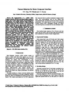
Consider a toy example in Figure 1.
This work is supported in part by a grant from Networks of Centers of Excellence/Institute for Robotics and Intelligent Systems, a grant from Institute for Robotics and Intelligent Systems/Precarn, and a grant from Natural Sciences and Engineering Research Council of Canada.
Philip S. Yu IBM T.J. Watson Research Center
[email protected]
Given “Credit Card” table and “Transaction” table, suppose we want to select features that are relevant to determine whether certain credit card is in good standing or not. A straight-forward method would join these tables on the common feature “Account No”, resulting in a joined table with 8 records and 9 attributes. Each feature can then be examined against the class attribute in the joined table. ■ Several problems arise with this approach. Firstly, as the join operation is expensive and there is blow-up in the data size, it is a waste in both time and space as many features will be removed by subsequent feature selection. Secondly, unnecessary details are revealed which violates the data privacy constraint, thus is undesirable. In addition, there are cases where learning is done on some query results defined with each user specification, e.g., to study personal behaviors, user may want to join the two example tables on persons’ names. It is thus impossible to materialize the joined result once and use it for all subsequent learning. In this paper, we propose a way to perform feature selection without join. We observe that a feature selection algorithm is essentially a computational solution that measures the class relevance of all features. For typical relevance measures, all information required in the computation is the class distribution associated with each feature. If the class information can be propagated to all data sources, it is easy to evaluate all features locally. Thus, instead of evaluating all features in a central table, we push the class labels into each individual data source. In other words, we push the process of feature selection ahead of the join operation.
2. Related Works In multi-relational learning such as [1,10,13], the target entity is an “object”, which is one entry in the target table. Features in all non-target tables are properties of the target object. However, the problem we are dealing with is conceptually different. We regard each entry in the final joined table as our target entity, i.e., classification is defined on joined instances. A number of surveys on feature selection methods are available [3,8]. In general, it’s a process that chooses an optimal subset of features according to certain criterion
Credit Card
Acc. No
Card Holder
Class
Trans. No
Acc. No
Date
Customer
Type
Amount
C1
A1
Mary
Good
1
A1
02/12’02
Michael
transfer
100.00
C2
A1
Michael
Good
2
A1
03/03’03
Michael
withdraw
200.00
C3
A2
Helen
Bad
3
A2
05/20’02
John
deposit
390.98
C4
A2
John
Good
4
A2
11/01’03
Helen
transfer
34.00
Credit Card Table
Transaction Table
Figure 1. Example Database with Many-to-Many Relationship [7]. Previous works on feature selection focused on developing evaluation criteria and search strategies, given one flat table with a set of features. Not much work is done when it comes to feature selection across multiple relations, other than the intuitive join approach. Sampling is another technique that is often used for scalability. However, as it only operates on a portion of the original data, the results are only approximations. Also, it does not address the data privacy issue at all. As one work that is close to ours, the VFREL algorithm proposed in [5] made use of feature selection to reduce the dataset size before passing the flattened (joined) data to a propositional learner. At each iteration, a small sample of the flattened database is used to eliminate features that are most likely to be irrelevant. That is, they still perform join on a portion of data at each step in order to select features. Our work differs as we eliminated the need of join before feature selection. In addition, we also address the data privacy problem while there is no such concern in their context. The idea of information propagation across multiple relations has been explored [13]. However, they propagated IDs of target records, which may be of arbitrarily large size. And they need to do propagation in each iteration of building the classifier. We propagate class labels with a size equal to the number of classes (typically very small in classification). Once the class label is propagated to each table, all evaluation is done locally and there’s never need to propagate again.
3. Algorithm Overview Figure 2 compares our approach with the existing approach. With our framework, feature selection is done through class propagation where class distribution information is propagated from the class table to other tables without join. By pushing feature selection ahead, we only need to join a much smaller subset of features at a later stage, thus the algorithm is more scalable and data privacy is protected. In order to measure the relevance of features, typical
Simple Approach Join (all features)
Feature Selection Classification
Our Approach Class Propagation Feature Selection Join (with subset of features) Classification
Figure 2. Work Flow Overview measures such as information gain [9] and gini index [2] are defined based on the relative frequency of each class. Everything that is needed for calculating these measures is contained in the projection of the examined feature values and their class distribution. Such projection has been referred to as “AVC (Attribute-Value-Class label) set” in [4]. The size of such AVC set is proportional to the number of distinct values in each attribute. To obtain such AVC values, the only data structure that needs to be propagated is the class distribution information. This observation leads to the first and the core part of our algorithm, class propagation. The operations after class propagation are rather standard, including feature selection, join and classification. As our focus is to study the effect of class propagation, we simply made use of some commonlyused existing methods. We do not intend to introduce a new feature selection or classification algorithm. Rather, we provide a method to perform feature selection directly on multiple data sources. Since we measure the relevance of features in the same way as it is done on the joined table, it is guaranteed the resulted feature set is exactly the same as would be produced by joining the databases. In the next section, we will focus on details of class propagation.
4. Class Propagation To propagate class information, we maintain a data structure at each data source, named “ClsDis” (class
distribution vectors), in the form of “” where n is the total number of classes. Each count in the vector represents the number of instances of the corresponding class in the joined table. Operations on such class vectors are performed on each corresponding pair of class counts. For some operator ‘⊗’ and two vectors V: and V’: , V ⊗ V’=. (e.g., *==)
4.1 An example with a 2-table database Consider our toy example database in Figure 1. Credit Card table contains the class label (credit standing “good” or “bad”). We consider the query where we need to join the tables on “Acc. No” for classification. Step 1. Initialization In the class table, if a tuple has class i, its class vector is initialized such that counti=1 and countj=0 where j≠ i. For non-class tables, all counts of the class vectors are initialized to 0s. Step 2. Forward Propagation Class propagation starts from the class table. Since we are joining on the attribute AccNo, for each tuple in Transaction table with AccNo = Ai, its “ClsDis” is the aggregation of class counts in Credit Card table with the same AccNo. This results in the Transaction table with propagated “ClsDis” as shown after step 2 in Figure 3. Note the total class count in Transaction table have reflected the effect of join on both tables.
Step 3. Backward Propagation Then we need to propagate back from Transaction table to Credit Card table, as the class counts in Credit Card table have not reflected the join. Consider a tuple T with AccNo=Ai in Credit Card table. T will join with all the tuples in Transaction having this account number. Let V be the aggregated class counts for such tuples in Transaction. V is also the aggregated class counts over all tuples in Credit Card with this AccNo. T is one of such tuples. We need to redistribute V among such tuples in Credit Card according to their shares of class counts in Credit Card table. As an example, the third tuple in Credit Card table has “AccNo=A2” and gets the new “ClsDis” as a result of *(/), since the aggregated “ClsDis” with “AccNo=A2” is in Transaction table, the original class vector is in this entry of Credit Card table, and the aggregated class vector with this account number in Credit Card table is . The final results are shown after step 3 in Figure 3. After propagation, all tables contain the same aggregated class count, which is the same as if we have joined the tables. This is also why we need to propagate in a backward direction, so that the effect of join is reflected in all tables. (We omit the formal proof due to the space limit.)
4.2 General Scenarios In general, we can deal with datasets with acyclic relationships among tables, i.e., if each table is a node and related tables (share join predicate) are connected
Credit Card
Acc. No
Card Holder
ClsDis
Credit Card
Acc. No
Card Holder
ClsDis
C1
A1
Mary
C1
A1
Mary
C2
A1
Michael
C2
A1
Michael
C3
A2
Helen
C3
A2
Helen
C4
A2
John
C4
A2
John
Credit Card Table
Total:
Credit Card Table Total: Step 2: propagate forward
Trans. No
Acc. No
Date
Customer
Type
Amount
ClsDis
1
A1
02/12’02
Michael
transfer
100.00
2
A1
03/03’03
Michael
withdraw
200.00
3
A2
05/20’02
John
deposit
390.98
4
A2
11/01’03
Helen transfer Transaction Table
34.00
Total:
Figure 3. Class Propagation on the Example Database with 2 tables
Step 3: propagate backward
by edges, the resulted graph should be acyclic. Under this assumption, for cases with more than two tables and complex schemas, class vectors are propagated in the depth-first order from the class table. This process may include both forward (when propagating from table at a higher level downward) and backward (from a lower table upward) propagations. The last table contains class information aggregated from all tables. To ensure all other tables contain the same information, class vectors are then propagated back in one pass.
5. EXPERIMENTAL RESULTS 5.1 Experiment Settings We compared the performance of feature selection on multiple tables through class propagation (CP algorithm) with feature selection on joined table (Join algorithm). Since they both return the same set of features, we only need to compare their running time. We also examined the effect of feature selection on classification. We rank features according to information gain, as it is one of the most often used evaluation criteria. Then we select a top percentage of features. When join is needed, it is done as a standard database operation by using Microsoft SQL Server. As this software has a limit on the number of attributes in any single table (1024), when the dataset exceeds this limit, we wrote an alternative join program which is a simple implementation of the nested loop join [11]. For classification, we implemented RainForest [4] to build a decision tree classifier, since decision trees are reasonably good in performance and easy to comprehend [2,9]. RainForest has been shown to be a fast classifier on large scale data, where the traditional decision tree classifier C4.5 [9] can not be used when data is very large or has very high dimensions. All implementations are written in C++. Experiments were carried out on a PC with 2GHz CPU and 500M main memory running Windows XP.
5.2 Datasets Mondial dataset is a geographic database that contains data from multiple geographical web data sources. We obtained it in the relational format online [12]. Our classification task is to predict the religion of a country based on related information contained in multiple tables. We consider all religions which are close to Christian 2 as positive class and all other religions as negative class. We ignored tables that only consist of 2
Armenian Orthodox, Bulgarian Orthodox, Christian, Christian Orthodox, Eastern Orthodox, Orthodox, Russian Orthodox
geographic information. Finally we have 12 tables, the number of attributes ranges from 1 to 5 and all tables have less than 150 records with two exceptions (one table has 1757 records and another has 680 records). About 69% of data is negative and 31% is positive. 10 fold cross validation is used on this dataset. Yeast Gene Regulation dataset was deduced from KDD Cup 2002 task 2 [6]. We obtained 11 tables that contain information about genes (detailed descriptions are omitted due to space limit). The biggest table contains keywords produced from abstracts that discuss related genes by using standard text processing techniques (removing stopwords, word stemming). It has 16959 records with 6043 attributes. The class table has 3018 records with the class label, which represents the effect of gene on the activity level of some hidden system in yeast (“has changes”(1%), “has controlled changes”(2%), “no changes”(97%)). Separated training and testing samples are used as provided in KDD Cup.
5.3 Experiment Results Table 1 shows the running time on each stage of both algorithms and classification results on both datasets. Note that the step for building the classifier is exactly the same for both approaches, since we have the same joined data at this stage. Also, when 100% features are selected, i.e., there is no feature selection, both algorithms degrade to the same method. It can be seen that our CP algorithm runs much faster than the join approach. The breakdown of the running time shows that the major gain is on the time needed for joining the data. As explained earlier, the join approach has to join a much larger dataset, taking a long time, whereas we only need a fraction of that time joining much less features. The experiments also show that our class propagation process is very fast and efficient, giving us the benefit of doing feature selection before join at very little cost. For Mondial dataset, the accuracy difference is significant between 40% and 50% feature subsets, suggesting that some attributes are very helpful in identifying the class label, although they may not be ranked very high. In general, when more of data privacy is preserved (with less features revealed to other parties), classification accuracy starts to decrease. However, if the user has very strict privacy requirements, then we can only select less features to satisfy such constraint. For Yeast Gene dataset, a small number of features provide very accurate classification and all other features are irrelevant. It is shown by the perfect accuracy starting from 5% feature subset. When more features are selected, it simply prolongs the running time without changing accuracy. On the other hand, the
spent for feature selection itself. However, this is not the case for our CP algorithm, as the time of our feature selection is much shorter and the total running time always benefits from feature selection.
total running time of the Join approach without feature selection is less than the total time with 10% or more feature selection. This is because the effect of feature selection on classification time is offset by the time
Running Time (seconds)
Join
CP
Mondial Dataset
Yeast Gene Dataset
Features selected (%)
Features selected (%)
20
30
40
50
100
5
10
20
50
100
Join
137
137
137
137
137
1099
1099
1099
1099
1099
Feature Selection
9.1
10.6
11.7
14.7
0
1265
1587
1879
2549
0
Building Classifier
32.1
41.2
50.1
53.5
119
50
176
370
1001
1739
Total
178.2
188.8
198.8
205.2
256
2414
2862
3348
4649
2838
Class Propagation
1.2
1.2
1.2
1.2
0
9
9
9
9
0
Feature Selection
0.4
0.5
0.5
0.5
0
130
144
158
228
0
Join
1
1
1
1
137
67
118
226
589
1099
Building Classifier
32.1
41.2
50.1
53.5
119
50
176
370
1001
1739
Total
34.7
43.9
52.8
56.2
256
256
447
763
1827
2838
71.5
72.1
69.2
98.1
98.5
100
100
100
100
100
Accuracy (%)
Table 1. Comparison of Running Time / Accuracy
6. DISCUSSION In this paper, we present a way of selecting features in multiple data sources without join. With a clever propagation of class vectors, each local data source receives the same class distribution information as produced by a join approach. Features can then be evaluated locally. Thus the resulted feature selection scheme is highly scalable, while limiting the amount of information disclosed to other data sources. The idea of class propagation can be used to develop more complex feature selection solutions. For example, we can incorporate the privacy constraints directly into feature evaluation by defining privacy score (from 0 to 1) for each feature. Features with higher privacy scores should have less chance to be selected. Since such score is available at each local data source, we can design some complex measure to evaluate the features based on not only the relevance to the class label, but also such privacy constraints.
7. REFERENCES [1] A. Atramentov, H. Leiva and V. Honavar, A MultiRelational Decision Tree Learning Algorithm – Implementation and Experiments. ILP 2003. [2] L. Breiman, J.H. Friedman, R.A. Olshen and C.J. Stone, Classification and Regression Trees. Wadsworth: Belmont, 1984.
[3] M. Dash and H. Liu, Feature Selection for classification. Intelligent Data Analysis – An International Journal, Elsevier, 1(3), 1997. [4] J. Gehrke, R. Ramakrishnan and V. Ganti, RainForest: a Framework for Fast Decision Tree Construction of Large Datasets. The 24th VLDB conference, 1998. [5] G. Hulten, P. Domingos and Y. Abe, Mining Massive Relational Databases, 18th International Joint Conference on AI - Workshop on Learning Statistical Models from Relational Data, Acapulco, Mexico, 2003. [6] KDD Cup 2002, http://www.biostat.wisc.edu/~craven/kddcup/train.html [7] H. Liu and H. Motoda, Feature selection for knowledge discovery and data mining. Kluwer Academic Publishers, 1998. [8] L. C. Molina, L. Belanche and A. Nebot, Feature Selection Algorithms: A Survey and Experimental Evaluation. ICDM 2002. [9] J.R. Quinlan, C4.5: Programs for Machine Learning. Morgan Kaufmann, 1993 [10] J. R. Quinlan and R. M. Cameron-Jones. FOIL: A midterm report. In Proc. 1993 European Conf. Machine Learning, Vienna, Austria, 1993. [11] R. Ramakrishnan and J. Gehrke, Database Management Systems. McGraw-Hill, 2003. [12] The Mondial Database, http://dbis.informatik.unigoettingen.de/Mondial/#Oracle [13] X. Yi, J. Han, J. Yang, and P. Yu. Crossmine: efficient classification across multiple database relations. ICDE 2004.