1
ImageAdmixture: Putting Together Dissimilar Objects from Groups Fang-Lue Zhang, Ming-Ming Cheng, Member, IEEE, Jiaya Jia, Senior Member, IEEE, and Shi-Min Hu, Member, IEEE, Abstract—We present a semi-automatic image editing framework dedicated to individual structured object replacement from groups. The major technical difficulty is element separation with irregular spatial distribution, hampering previous texture and image synthesis methods from easily producing visually compelling results. Our method uses the object-level operations and finds grouped elements based on appearance similarity and curvilinear features. This framework enables a number of image editing applications, including natural image mixing, structure preserving appearance transfer, and texture mixing. Index Terms—natural image, structure analysis, texture, image processing
F
1
I NTRODUCTION
Image analysis and editing provide an important approach to producing new content in computer graphics. We propose here a dedicated system for users to replace structured objects selected from groups while preserving element integrity and providing visual compatibility. It proffers an unconventional way to create new image content with structured objects, even when they are irregularly arranged. The objects are allowed to be dissimilar in appearance and structure, as shown in Fig. 1. Image and texture synthesis from multiple exemplars have been explored in previous work. Pixel-level texture approaches make use of similar statistical properties to generate new results [3], [8], [41]. Patch-based texture synthesis [12] is another set of powerful tools to selectively combine patches from different sources [21]. Recently, Risser et al. [32] employed multi-scale neighborhood information to extend texture synthesis to structured image hybrids. They are useful for creating new image or texture results based on examples. These methods are general; but in the context of object replacement within groups, they may not be able to produce visually plausible effects without extensive user interaction. Grouped elements can be rapidly and integrally perceived by the human visual system (HVS) [19], which indicates only considering pixel- or patch-level operations may not be enough to understand the individual structured element properties. Our system is composed of object-level editing algorithms and does not assume any particular texture form or near-regular patterns. Our major objective is to deal with natural images containing piled or stacked objects, which are common in real scenes, from the individual perspective. • F.L. Zhang, M.M. Cheng and S.M. Hu are with TNList, Tsinghua University, Beijing, China. E-mail:
[email protected],
[email protected] and
[email protected]. • J. Jia is with the Chinese University of Hong Kong, Hong Kong. E-mail:
[email protected].
Fig. 1. A mixture created by our approach. Cookies are replaced by plums while maintaining a visually plausible structure.
The naturalness of element replacement depends on the compatibility of input and the result structures. It is measured in our system by the element-separability scores, combining curvilinear features and multi-scale appearance similarity. Objects are extracted based on these metrics, with initial center detection followed by a Dilate-Trim algorithm to form complete shapes. Our method also finds suitable candidates for element replacement to ensure the result quality. Our main contribution lies in an object-level manipulation method without regularity assumption and on a new scheme to measure object structure compatibility.
2
R ELATED W ORK
Image composition is a well studied problem in computer graphics. Early work of Porter and Duff [31] used an alpha matte to composite transparent objects. Recent advance in alpha matting [38] made it possible to generate natural and visually plausible image composite with global or local operation. For our problem, directly apply alpha matting to replace one object by another can generate visual artifacts when illumination conditions vary. Poisson blending [30]
2
(a) Input image
(b) Appearance similarity
(c) Element-separability
(d) Detected elements
(e) Replacement result
Fig. 2. Framework: (a)the user selects one point, and our system generates an appearance similarity map (b), informative for finding objects in groups. After curvilinear feature refinement, we obtain the separability map (c). In (d), yellow dots represent elements detected by our method, with their core regions marked in blue. A replacement result is shown in (e).
and its variations reduce color mismatching by computation in the gradient domain. Farbman et al. [14] achieved similar composition results efficiently. Research efforts have also been made to select candidates for composition from image database [23] or internet images [9]. Such methods minimize composition artifacts while keeping the original object shape complete. In our problem, it is essential to seek proper image content to replace items in groups via compatible structures. We also do not simply copy the whole region to the target image for blending. There are procedures to refine boundaries to improve the visual quality of the results when in common situations that the found source and target objects are diverse in structure.
texture from multiple examples. The mixed area produced by these methods tends to have similar statistics or visual characteristics to the source. In RepFinder [10], although element replacement can be conceptually achieved, strict shape similarity has to be enforced and there is no consideration of object consistency. In contrast, our work places elements from different groups, where the visual characteristics are allowed to be greatly different. Recently, Ma et al. [28] mixed objects by modeling the combination of individual elements and their distributions. However, this method cannot solve our problem and requires users to manually produce the source elements.
Our work is also related to example-based texture synthesis. Efros and Leung [13] proposed a non-parametric pixel-wise method to synthesize new texture from a user provided example, trying to preserve as much local structures as possible. The efficiency and capability were improved by tree-structured vector quantization [40], global optimization [20], and multi-scale synthesis [15], [24]. Patch based approaches [12], [21] form another important line for texture synthesis with the main idea being to find an optimal seam between adjacent patches. Mask images [29], [43] and feature maps [34], [42] can be used to guide texture synthesis. These methods provide a powerful tool for creating visually similar content from a few examples [39], but none of them can be applied directly to natural images for separating grouped elements, and then replacing objects in a visually plausible way. The main challenge is that the underlying structured element regions may be changed in this process, as demonstrated in Fig. 1.
3
Synthesis and analysis may also be done at the texel level. Dischler et al. [11] manually segmented texture into particles. Automatic methods [1], [37] extracted texels based on sub-tree matching in low-level segmentation. They can extract texels that are significantly occluded. It is however time-consuming and can fail when segmentation is unreliable for grouped elements. Ijiri et al. [18] showed how to manipulate elements which are distributed near-regularly. Combining features or visually meaningful content from different samples, i.e. image/texture mixing, allows users to produce results with large variation. In prior work such as image hybrids [32], Risser et al. synthesized image hybrids from exemplars. Other methods [3], [8], [41] generated new
G ROUPED E LEMENTS A NALYSIS
Replacing content within groups of objects is challenging, since our human vision system (HVS) is sensitive to scene integrity, shape compatibility, illumination consistency, etc. Our method first finds separable objects in the target image based on element-separability analysis, which captures the global distribution of grouped elements. An elementseparability map is then generated, indicating where to find individual elements. We use a Dilate-Trim method to extract element boundaries. 3.1 Multi-scale Appearance Similarity
The first stage of our method is to detect inherent appearance similarity in the given target group, which helps analyze element distribution. The necessity of doing this has been observed in other texel analysis work [7], [16], [26]. Our system requires the user to choose a point p0 to specify a key appearance feature of the objects to be extracted, as shown in Fig. 2(a). We use multi-scale descriptors [32] to measure how this point (together with its neighbors at different scales) matches other parts of the given image, which eventually lets us know the possible distribution of elements in the group. We build a Gaussian pyramid. The finest level is the original image. Each coarser level is smoothed and down-sampled by a factor of 2. The descriptor vector of pixel p at each level has 75D after stacking all pixels in a 5 × 5 square neighborhood window in a vector considering 3 colors. The vector at each level
3
matching. This procedure yields local curve magnitude mp for each pixel p (shown in Fig. 3(b)), the length lC of each curve C, and corresponding curve points. Based on these, we define saliency for each curve C as Sc (C) = N (
1 ∑ mp ) · N (lC ), |C|
(1)
p∈C
(a) The group
(b) Local curve magnitude
(c) Curve saliency [6]
(d) Our result
Fig. 3. Comparison of curvilinear feature detection methods. The local curve magnitude method [36] and the message-passing based curve saliency map [6] are shown in (b) and (c). Our result is shown in (d).
is projected to only 6D by principal component analysis (PCA). If the total number of levels is L, concatenating all 6D vectors in the pyramid yields a 6L-D final descriptor. Our experiments show that L = 4 is generally a good choice. Using a larger L can capture a wider range of visual features with higher computational costs. We measure the Euclidean distances between the descriptor vector for p0 and those for other pixels, which yield an appearance similarity map Sa with the same size as image I. For each pixel p, its value is denoted as Sa (p, p0 ). An example is shown in Fig. 2(b). Dark pixels are with high similarity with p0 with respect to multiscale neighbors.
3.2
Robust Curvilinear Features
Curvilinear features [42], such as edges and ridges, which primarily describe object boundaries in natural images, provide strong evidence for finding similar objects. As shown in Fig. 3(b), curve magnitudes in natural images are influenced by object occlusion, illumination variation, local appearance change, etc. The curve detection method [36] depends on local curve magnitudes and may find it difficult to maintain boundary continuity. Perception study shows that long coherent curves are perceptually salient to HVS [5]. Bhat et al. [6] employed a message passing scheme to find such curves. Albeit effective, it occasionally breaks object boundaries, hindering object extraction and transplantation. We propose a simple method to define curve saliency according to curve length and average local curve magnitude. Our approach starts by finding curvilinear structures [36], which link confident curve points using orientation
∑ 1 where |C| p∈C mp is the average gradient magnitude along C, as |C| is the number of pixels in C. N (∗) is a Gaussian normalization function [2], keeping 99% of the values in range [0, 1] after conversion. Sc (C) has two terms, so that a long curve with large saliency is favored. Combining Sc (C) for all curves C, we form a curve saliency map Sc . Each pixel p has a value denoted Sc (p). As shown in Fig. 3(d), our curve saliency map Sc (I) contains more informative structures than those of Bhat et al. [6], and exhibits coherent curvilinear features. In addition, our saliency definition is suitable for user interaction because it only takes a few milliseconds of computation for a typical natural image, while in [6], tens of seconds are needed.
3.3 Separation of Structured Objects
The position of each element in the target group is a potential place to put a new item. Both the appearance similarity and curvilinear features are important cues for the HVS. We estimate an element separability map (ESmap for short) to identify element centers, defined as S(p) = Sc (p) − ωSa (p, p0 )
(2)
where Sc (p) and Sa (p, p0 ) are the curve saliency and appearance similarity values for p respectively. The weight ω is set to 1 in experiments. A smaller ω makes the curvilinear features more readily separate neighboring elements, under the risk of partitioning one element into two. The simple ES map is vital for understanding the global distribution of all elements. Regions with high-similarity of appearance will present local peaks in the map, while still being outlined by the curvilinear features. With this map, elements close to each other can be quickly separated, as shown in Fig. 2(c). We perform clustering-based segmentation in the ES map, by thresholding the map and taking each connected region as an individual segmented component. The default threshold is set to 0.5. If the threshold is too small, neighboring elements with unclear boundaries could be recognized as one. In the segment map Ms , each region is basically an element’s core body. The region centroids can thus be found, highlighted in yellow in Fig. 2(d). The region boundaries are however coarsely determined, and will be refined in the next step.
4
(a) Element
(b) Result of snake
(c) Our result
Fig. 5. Comparison of the active contour method and our Dilate-Trim. (a) Separable elements with their core regions. (b) Mask from active contour. The external energy is calculated by Equation (3)(c) Our automatically produced result.
3.3.1
Comparison with other methods
2.1D-texels: The element extraction result of 2.1D-texels [1] is shown in Fig. 4(a) for comparison. This method applies matching in the segmentation tree to achieve unsupervised element extraction. As the elements may not have similar subtrees, missing objects and false detection can be more seriously resulted for this challenging example. Region of Dominance: Region of Dominance (RoD) was employed in [25] to extract texels in near-regular textures based on normalized cross correlation (NCC). RoD is defined as the largest circle centered at the candidate peak of NCC. Due to search for dominant peaks, if two elements are very close, separation cannot be achieved, as shown in Fig. 4(b). Further, RoD does not provide the boundary information, which is nonetheless critical for our object transplantation in groups. RepFinder: RepFinder was proposed in [10] to detect approximately repeated elements in natural scenes. A Boundary Band Map(BBM) was employed to extract objects. However, because RepFinder relies on the shape similarity to extract objects, it fails when the grouped elements have different shapes, as shown in Fig. 4(c). Note that our method does not assume that the elements are regular in distribution and in appearance. The elementseparability analysis is applicable to examples that are challenging for near-regular texture methods, and provides a reliable object separation scheme in general. More results are shown in later sections. 3.3.2
Element Extraction by Dilate-Trim
Given the computed element centers, i.e., yellow dots in Fig. 4, we now refine each element’s boundary L by requiring it to have large gradient magnitude and small irregularity. The active contour model provides one way to solve this problem. The summed external energy term of every contour point is: ∫ ∑ Sc (p) Sc (p) EL = ds = , D(p)Sa (p, p0 ) + ϵ L D(p)Sa (p, p0 ) + ϵ p∈L (3) where ϵ is a small value to avoid division by zero and D(p) is the distance from pixel p to the corresponding
Algorithm 1 Extract an elementary region R by DilateTrim. Initialize R as one region in Ms in Section 3.3; Initialize R′ = ∅; while R − R′ > δ, where δ is a stopping value do R′ ← R; R ← Dilate(R); for every pixel p ∈ R do remove p from R, when Sc (p) < t(p); end for R ← largest connected region of R; end while
center point. However, as Fig. 5 shows, because the active contour method trades off between the contour smoothness and external energy distribution, it can not cover all the details. We thus use a Dilate-Trim method, sketched in Algorithm 1, to solve the problem progressively. Specifically, it iteratively dilates regions and then trims them until the added pixels are less than an adaptive threshold t(p) = S(p)/D(p). t(p) makes dilation be stopped for pixels with high separation confidence or distant enough from the center. The border gradually expands from the element center, and can evolve differently for various objects, suitable for forming irregular shapes. As Fig. 5 shows, in comparison with the active contours, our method can adaptively and more accurately update object boundaries, fitting our pursuit. Another popular choice for multi-label segmentation in element groups is by global optimization, such as graph cuts and watershed, taking the element centers as seeds. This scheme cannot handle pixels that do not belong to any of the elements. One example is shown in Fig. 6(a). Our method, on the contrary, considers individual elements starting from their centers, and thus can produce better shapes as shown in Fig. 6(b). Pixels are allowed to be not in any of the elements . 3.3.3 Choosing Suitable Elements
We perform Dilate-Trim for each element in the target image, exemplified in Fig. 2(a), containing a group of objects. Based on the results, our system allows the user to choose the element region to replace. Our method then finds a candidate region from the secondary image with similar curvilinear feature and compatible with the target gradient change. The similarity between the two images is measured by cross-correlation. We expand the target object boundary by a few pixels, creating a boundary band map [10]. Then we calculate cross correlation values between the target element and all regions in the secondary image on the bands. The two regions that yield the largest value are regarded as most compatible. If there are multiple objects to be processed, we repeat this selection process.
5
(a) 2.1D texels
(b) RoD
(c) RepFinder
(d) Our result
Fig. 4. Comparison of 2.1D texels [1], Region of Dominance (RoD) after NCC [16], RepFinder [10] and our method. Yellow dots are the detected element centers. region replace
a
boundary replace
c
b nearest neighbor search
BBM Search
d (a) Global optimization
(b) Dilate-Trim
Fig. 6. Global segmentation versus dilate-trim. (a) Result of multi-label segmentation. (b) Our result of dilate-trim on each element starting from its center.
4
Fig. 7. Element replacement. (a) Region extracted by Dilate-Trim. (b) Initially replacing RA by RB . (c) Our fi′ nal RA with boundary refinement on (b). (d) Boundary refinement by patch-based nearest neighbor search and replacement, which is visually less pleasing than (c).
E LEMENT R EPLACEMENT
To replace an element RA in image A by RB obtained from the secondary image B, object shape needs to be maintained with natural visual appearance change. This goal cannot always be achieved successfully when using gradient-domain image blending. We instead propose a patch searching strategy to retain visually compatible borders. The luminance is then transferred to produce final results. Poisson blending and tone mapping are useful tools in image composition. The need to keep object appearance in our problem, however, is beyond their capability. Firstly, these methods can drastically change the object color when the source and target images are quite different. Secondly, they cannot create natural boundaries for each replaced object, as shown in Fig. 1.
Neighbors
boundary(not to replace) boundary(to replace) inner region
Image not-in-region region mask
non-neighbor neighbor
Fig. 8. Three different areas in an object (left). In the boundary band to be refined, the mask only contain pixels inside the object (right). 4.1 Boundary Replacement
With the candidate region RB found in the secondary image B, as described in Section 3.3, we initially replace RA by
6
(a)
(b)
(c)
(d)
(e)
Fig. 9. Mixing elements: (a) target image; (b) ES-map; (c) detected elements; (d) secondary image; (e) mixing result.
RB , as shown in Fig. 7(b). RB , by definition, contains the most similar curvilinear feature as RA near boundary. Note that directly copying RB still causes visual artifacts. One intuitive way to improve it is by employing the nearest neighbor search, like PatchMatch [4], to refine the boundary of RB . However, as shown in Fig. 7(d), this method does not perform well enough when A and B do not have similar structures. We alternatively look for large intensity variation near boundaries of RB and RA . The updated region, denoted ′ as RA , is produced as ′
RpA =
(a) Before luminance transfer
(b) Luminance transfer result
Fig. 10. Results before and after luminance transfer.
4.2 Luminance transfer
{ B Rarg minq D(p,q)
p ∈ Ω(RA )
RpB
∩
A ∥∇B p − ∇p ∥ > T
otherwise
(4) ′ ′ where Ω(RA ) is the 5-pixel width boundary band of RA , B B as shown in Fig. 8. q can be any pixel in R , and ∥∇p − ∇A q ∥ measures difference in gradient. T is a threshold, set to 0.25 by default; our algorithm is insensitive to this value. D(p, q) is the distance between p and q, defined as
Finally, we approximate luminance from the original image, and transfer it to the result. Existing luminance transfer methods [22] mainly consider features and image structure. Since we already have the appearance similarity value Sa (p, p0 ) for every pixel indicating the difference between p and the user selected pixel p0 , we define a luminance score function L(p) for every pixel p: L(p) = Sa (p, p0 ) · (I¯NpA − I¯NpA ), 0
D(p, q) =
∥NqB
−
NpA ∥
+
α∥∇B q
−
∇A p ∥,
(5)
where NqB and NpA are masked local windows centered at q and p respectively. We use α = 1 in all our experiments to equally weight the two factors. Pixels p and q have to be close in both appearance and gradient to yield a small ′ D(p, q) along the region’s boundary Ω(RA ). To design NqB and NpA , square windows [33], [41] used in traditional texture synthesis are not appropriate when irregular boundaries exist. In our method, we only include pixels that are in region RA for reliable appearance matching, as illustrated in Fig. 8. So the overall object replacement can be summarized as a two-step process, which first copies pixels from RB to RA . Then part of the boundary (shown in orange on the left of Fig. 8(a)) is adjusted according to Equation (4) to improve appearance compatibility. Fig. 7(c) shows a result. In Equation (4), to obtain q w.r.t. minq D(p, q), we avoid time-consuming brute-force search in B and only keep candidate patches in RB that have small mean-color differences to NpA . We maintain the top 20% candidate patches for detailed comparison in Equation (4).
(6)
where NpA denotes the masked neighborhood of p in image A, and I¯NpA is the average intensity of pixels in NpA . L(p) can be either positive or negative, and is useful to change the pixel brightness depending on its sign. The final luminance transfer is performed for each pixel p using P ′ (p) = P (p) + λL(p),
(7)
where P (p) and P ′ (p) denote the pixel values before and after luminance transfer respectively, and λ controls the level of modification. Large λ yields strong highlight or shadow. We use λ = 0.75 in all our experiments. Results before and after luminance transfer are shown in Fig. 10.
5
A PPLICATIONS
AND
R ESULTS
In our algorithm implementation, the regions to operate on in the input images are segmented by grab-cut [35] if necessary. Then the target objects are separated as described in Section 3. The specified objects are replaced one by one using the method given in Section 4. On a PC with a CPU at 2.5GHz and 4GB RAM, the computation time is around 0.2 seconds for element analysis on a 640×480 image, and is about 20 milliseconds to replace each element.
7
Fig. 11. Structure preserving texture transfer: (left) target image and novel source texture; (right) texture transfer result.
[41]. Our approach is an alternative to this end. We first mix the two exemplars to create a new texture sample using the steps described in the paper. Each texton in the two textures is regarded as an atomic element. Then we perform the texture synthesis approach of Lefebvre and Hoppe [24] to generate a bigger image. One example is shown in Fig. 12, our method spatially blends two different kinds of texels in an element-wise manner, rather than providing a statistically uniform result similar to both inputs.
5.4 Limitations
Fig. 12. Texture mixing result. The user inputs two different images, based on which we produce a mixing result. A larger texture can be synthesized from the result.
5.1
Natural image examples
In real scenes, it is ubiquitous to see grouped elements with similar appearance. Our method is able to produce high quality element replacement results, as shown in Fig. 9. Unlike image composition techniques, our approach focuses on mixing visual features into the target area, while keeping the original structures, rather than overwriting them. Our image mixture approach is a complement to current image editing techniques.
There are a few difficulties that might influence the final result quality. Firstly, since we do not estimate any depth or layer information, our system cannot separate group objects well when this set of information is needed. We show an example in the left of Fig. 13, in which leaves overlay, destroying the latent integrity. The lack of depth information may also make object replacement not visually very pleasing when the 3D structure significantly varies in the two input images. Secondly, we require objects in the secondary image to have curvilinear compatible content to replace the original elementary region. As shown in the right of Fig. 13, when we replace the rectangular blocks by hexagonal stones, even considering the most compatible regions cannot preserve the visual integrity. The incomplete rocks inserted into the wall do not retain their correct geometric features. Finally, challenging objects like transparent or translucent glasses, cannot be properly handled in our system. Involving matting and image recognition will be our future work.
6
C ONCLUSION
In this paper, we have proposed a dedicated system to substitute structured elements within groups by others even 5.2
Structure preserving appearance transfer
Our method can also be applied to structure preserving appearance transfer in textured images. We only separate elements in the target image group using the boundary band map [10] to search for most compatible structures in the secondary texture image for replacement. Thereupon, the secondary image is not limited to grouped elements. One example is shown in Fig. 11, where we use a lichen texture to replace bricks, accomplishing the appearance transfer effect. The major difference between our approach and texture transfer [12], [17], [27] is that we can preserve the appearance and local structure of the original objects that remain in the admixture result. In Fig. 11, lichen appears to be growing on bricks. 5.3
Texture mixing
To blend texture, prior methods require input samples to have similar appearance or weak structural features [3], [8],
Fig. 13. Failure cases: (left) grouped objects with complicated 3D structure and layers; (right) object groups with incompatible structure.
8
Fig. 14. Further results. Each group has 3 images showing (from left to right) the source image, the secondary image, and our result respectively.
though they are dissimilar in appearance. Different levels of mixture are allowed in our system, preserving local structures. Our method requires a very small amount of user interaction. The analysis and other operations to separate objects are automatic. The drawback is that we do not consider layers and depth, which may be problem in some cases. But overall our method is powerful enough to handle many examples that are challenging for other approaches.
[7]
S. Brooks and N. Dodgson, “Self-similarity based texture editing,” ACM TOG, vol. 21, pp. 653–656, 2002.
[8]
G. Brown, G. Sapiro, and G. Seroussi, “Texture mixing via universal simulation,” in Proc. of Int. Workshop on Texture Analysis and Synthesis, 2005.
[9]
T. Chen, M. Cheng, P. Tan, A. Shamir, and S. Hu, “Sketch2Photo: internet image montage,” ACM TOG, vol. 28, no. 5, pp. 124: 1–10, 2009.
[10] M.-M. Cheng, F.-L. Zhang, N. J. Mitra, X. Huang, and S.-M. Hu, “Repfinder: Finding approximately repeated scene elements for image editing,” ACM TOG, vol. 29, no. 4, pp. 83:1–8, 2010.
ACKNOWLEDGMENTS We thank all the reviewers for their helpful comments. This work was supported by the National Basic Research Project of China (Project Number 2011CB302205), the Natural Science Foundation of China (Project Number 61120106007.
R EFERENCES [1] [2]
[3]
[4]
N. Ahuja and S. Todorovic, “Extracting texels in 2.1D natural textures,” in IEEE ICCV, 2007, pp. 1–8. S. Aksoy and R. Haralick, “Feature normalization and likelihoodbased similarity measures for image retrieval,” Pattern Recognition Letters, vol. 22, no. 5, pp. 563–582, 2001. Z. Bar-Joseph, R. El-Yaniv, D. Lischinski, and M. Werman, “Texture mixing and texture movie synthesis using statistical learning,” IEEE TVCG, vol. 7, no. 2, pp. 120–135, 2002. C. Barnes, E. Shechtman, A. Finkelstein, and D. B. Goldman, “PatchMatch: a randomized correspondence algorithm for structural image editing,” ACM TOG, vol. 28, pp. 24:1–24:11, 2009.
[11] J.-M. Dischler, K. Maritaud, B. Lvy, and D. Ghazanfarpour, “Texture particles,” Comput. Graph. Forum, vol. 21, pp. 401–410, 2002. [12] A. A. Efros and W. T. Freeman, “Image quilting for texture synthesis and transfer,” in ACM SIGGRAPH, 2001, pp. 341–346. [13] A. A. Efros and T. K. Leung, “Texture synthesis by non-parametric sampling,” in IEEE ICCV, 1999, pp. 1033–1038. [14] Z. Farbman, G. Hoffer, Y. Lipman, D. Cohen-Or, and D. Lischinski, “Coordinates for instant image cloning,” ACM TOG, vol. 28, pp. 67:1–9, 2009. [15] C. Han, E. Risser, R. Ramamoorthi, and E. Grinspun, “Multiscale texture synthesis,” ACM TOG, vol. 27, no. 3, pp. 1–8, 2008. [16] J. Hays, M. Leordeanu, A. Efros, and Y. Liu, “Discovering texture regularity as a higher-order correspondence problem,” Computer Vision–ECCV, pp. 522–535, 2006. [17] A. Hertzmann, C. E. Jacobs, N. Oliver, B. Curless, and D. H. Salesin, “Image analogies,” in ACM SIGGRAPH, 2001, pp. 327–340. [18] T. Ijiri, R. Mch, T. Igarashi, and G. Miller, “An example-based procedural system for element arrangement,” Comput. Graph. Forum, vol. 27, pp. 429–436, 2008. [19] B. Julesz, “Textons, the elements of texture perception, and their interactions.” Nature, vol. 290, no. 5802, p. 91, 1981.
[5]
W. Beaudot and K. Mullen, “How long range is contour integration in human color vision?” Visual Neuroscience, vol. 20, no. 01, pp. 51–64, 2003.
[20] V. Kwatra, I. Essa, A. Bobick, and N. Kwatra, “Texture optimization for example-based synthesis,” ACM TOG, vol. 24, pp. 795–802, 2005.
[6]
P. Bhat, C. Zitnick, M. Cohen, and B. Curless, “GradientShop: A gradient-domain optimization framework for image and video filtering,” ACM TOG, vol. 29, no. 2, pp. 1–14, 2010.
[21] V. Kwatra, A. Sch¨odl, I. Essa, G. Turk, and A. Bobick, “Graphcut textures: image and video synthesis using graph cuts,” ACM TOG, vol. 22, pp. 277–286, 2003.
9
[22] J.-F. Lalonde, A. Efros, and S. Narasimhan, “Estimating natural illumination from a single outdoor image,” in IEEE ICCV, 2009, pp. 183 –190. [23] J.-F. Lalonde, D. Hoiem, A. A. Efros, C. Rother, J. Winn, and A. Criminisi, “Photo clip art,” ACM TOG, vol. 26, 2007.
Fang-Lue Zhang received his BS degree from the Zhejiang University in 2009. He is currently a PhD candidate in Tsinghua University. His research interests include computer graphics, image processing and enhancement, image and video analysis and computer vision.
[24] S. Lefebvre and H. Hoppe, “Parallel controllable texture synthesis,” ACM TOG, vol. 24, pp. 777–786, 2005. [25] Y. Liu, R. Collins, and Y. Tsin, “A computational model for periodic pattern perception based on frieze and wallpaper groups,” IEEE TPAMI, vol. 26, no. 3, pp. 354 –371, 2004. [26] Y. Liu, J. Wang, S. Xue, X. Tong, S. Kang, and B. Guo, “Texture splicing,” Comput. Graph. Forum, vol. 28, no. 7, pp. 1907–1915, 2009. [27] Y. Liu, W.-C. Lin, and J. Hays, “Near-regular texture analysis and manipulation,” ACM TOG, vol. 23, pp. 368–376, 2004. [28] C. Ma, L.-Y. Wei, and X. Tong, “Discrete element textures,” ACM TOG, vol. 30, pp. 62:1–62:10, August 2011. [29] W. Matusik, M. Zwicker, and F. Durand, “Texture design using a simplicial complex of morphable textures,” ACM TOG, vol. 24, no. 3, pp. 787–794, 2005.
Ming-Ming Cheng received his BS degree from the Xidian University in 2007. He is currently a PhD candidate in Tsinghua University. His research interests include computer graphics, computer vision, image processing, and sketch based image retrieval. He has received a Google PhD fellowship award, an IBM PhD fellowship award, and a “New PHD Researcher Award” from the Chinese Ministry of Education. He is a member of the IEEE.
[30] P. P´erez, M. Gangnet, and A. Blake, “Poisson image editing,” ACM TOG, vol. 22, pp. 313–318, 2003. [31] T. Porter and T. Duff, “Compositing digital images,” ACM SIGGRAPH, vol. 18, no. 3, pp. 253–259, 1984. [32] E. Risser, C. Han, R. Dahyot, and E. Grinspun, “Synthesizing structured image hybrids,” ACM TOG, vol. 29, pp. 85:1–6, 2010. [33] L. Ritter, W. Li, M. Agrawala, B. Curless, and d. Salesin, “Painting with texture,” EGSR, pp. 371–377, 2006. [34] A. Rosenberger, D. Cohen-Or, and D. Lischinski, “Layered shape synthesis: automatic generation of control maps for non-stationary textures,” ACM TOG, vol. 28, no. 5, p. 107, 2009. [35] C. Rother, V. Kolmogorov, and A. Blake, ““GrabCut”: interactive foreground extraction using iterated graph cuts,” vol. 23, no. 3, pp. 309–314, 2004. [36] C. Steger, “An unbiased detector of curvilinear structures,” IEEE TPAMI, vol. 20, no. 2, pp. 113–125, 1998. [37] S. Todorovic and N. Ahuja, “Texel-based texture segmentation,” in IEEE ICCV, 2009, pp. 841–848.
Jiaya Jia received the PhD degree in Computer Science from Hong Kong University of Science and Technology in 2004 and is currently an associate professor in Department of Computer Science and Engineering at the Chinese University of Hong Kong (CUHK). He was a visiting scholar at Microsoft Research Asia from March 2004 to August 2005 and conducted collaborative research at Adobe Systems in 2007. He leads the research group in CUHK, focusing specifically on computational photography, 3D reconstruction, practical optimization, and motion estimation. He serves as an associate editor for TPAMI and as an area chair for ICCV 2011. He was on the program committees of several major conferences, including ICCV, ECCV, and CVPR, and co-chaired the Workshop on Interactive Computer Vision, in conjunction with ICCV 2007. He received the Young Researcher Award 2008 and Research Excellence Award 2009 from CUHK. He is a senior member of the IEEE.
[38] J. Wang and M. F. Cohen, “Image and video matting: a survey,” Found. Trends. Comput. Graph. Vis., vol. 3, pp. 97–175, 2007. [39] L. Y. Wei, S. Lefebvre, V. Kwatra, and G. Turk, “State of the art in example-based texture synthesis,” Eurographics, State of the Art Report, 2009. [40] L.-Y. Wei and M. Levoy, “Fast texture synthesis using tree-structured vector quantization,” in SIGGRAPH, 2000, pp. 479–488. [41] L. Wei, “Texture synthesis from multiple sources,” in ACM SIGGRAPH Sketches and Applications, 2003, pp. 1–1. [42] Q. Wu and Y. Yu, “Feature matching and deformation for texture synthesis,” ACM TOG, vol. 23, no. 3, pp. 364–367, 2004. [43] J. Zhang, K. Zhou, L. Velho, B. Guo, and H. Shum, “Synthesis of progressively-variant textures on arbitrary surfaces,” ACM TOG, vol. 22, no. 3, pp. 295–302, 2003. [44] D. Aiger, D. Cohen-Or, and N. J. Mitra, “Repetition maximization based texture rectification,” Comput. Graph. Forum (EG 2012 Proceedings), vol. 31, no. 2, 2012. [45] M.-M. Cheng, “Curve structure extraction for cartoon images,” in Joint Conference on Harmonious Human Machine Environment, 2009, pp. 13–20.
Shi-Min Hu received the PhD degree from Zhejiang University in 1996. He is currently a chair professor of computer science in the CS department, Tsinghua University, Beijing. His research interests include digital geometry processing, video processing, rendering, computer animation, and computer-aided geometric design. He is on the editorial board of Computer Aided Design. He is a member of the IEEE.