The Author(s) BMC Bioinformatics 2017, 18(Suppl 3):53 DOI 10.1186/s12859-017-1464-8
R ESEA R CH
Open Access
Pysim-sv: a package for simulating structural variation data with GC-biases Yuchao Xia, Yun Liu, Minghua Deng* and Ruibin Xi* From The Fifteenth Asia Pacific Bioinformatics Conference Shenzhen, China. 16–18 January 2017
Abstract Background: Structural variations (SVs) are wide-spread in human genomes and may have important implications in disease-related and evolutionary studies. High-throughput sequencing (HTS) has become a major platform for SV detection and simulation serves as a powerful and cost-effective approach for benchmarking SV detection algorithms. Accurate performance assessment by simulation requires the simulator capable of generating simulation data with all important features of real data, such GC biases in HTS data and various complexities in tumor data. However, no available package has systematically addressed all issues in data simulation for SV benchmarking. Results: Pysim-sv is a package for simulating HTS data to evaluate performance of SV detection algorithms. Pysim-sv can introduce a wide spectrum of germline and somatic genomic variations. The package contains functionalities to simulate tumor data with aneuploidy and heterogeneous subclones, which is very useful in assessing algorithm performance in tumor studies. Furthermore, Pysim-sv can introduce GC-bias, the most important and prevalent bias in HTS data, in the simulated HTS data. Conclusions: Pysim-sv provides an unbiased toolkit for evaluating HTS-based SV detection algorithms. Keywords: Copy number variation, Translocation, Breakpoints, Next-generation sequencing
Background Structural variations (SVs) are genomic variations that lead to structure changes of a donor genome. Indels, copy number variations (CNV) and genomic rearrangements are all subclasses of SVs. Many researches revealed that SVs are wide-spread in normal human populations [1, 2] as well as in cancer genomes [3–5]. High-throughput sequencing (HTS) has become a major platform for SV detection and a number of algorithms have been developed for SV detection with HTS data [6]. In genome studies based on HTS data, an important problem is to benchmark performances of various algorithms in different scenarios. The performance of an algorithm depends on its design, its implementation as well as quality and features of the sequencing data. An ideal method for
*Correspondence:
[email protected];
[email protected] School of Mathematics Science and Center for Statistical Science, Peking University, Yiheyuan Road 5, 100871 Beijing, China
benchmarking is by sequencing and subsequent experimental validation, but this method is expensive, labor intensive and time-costing. Thus, simulation of HTS data becomes a powerful and cost-effective alternative way for benchmarking genomic variation detection algorithms. Usually, benchmarking HTS-based SV detection algorithms by simulation involves (1) generation of genomes containing simulated SVs and (2) simulation of HTS short reads based on the genomes with simulated SVs. To approximate real HTS data, the generated genomes should be similar to real genomes and the simulated HTS data should contain various sequencing errors and biases. Since tumor samples often contain normal contaminations and heterogeneous subclonal tumor cells, simulation data of tumor genomes should contain normal contamination and/or multiple subclonses. There are several available SV simulation packages including RSVsim [7], SCNVsim [8], VarSim [9], IntSIM [10] and SInC [11]. These packages provide great resources for the community. However, as far as we
© The Author(s). 2017 Open Access This article is distributed under the terms of the Creative Commons Attribution 4.0 International License (http://creativecommons.org/licenses/by/4.0/), which permits unrestricted use, distribution, and reproduction in any medium, provided you give appropriate credit to the original author(s) and the source, provide a link to the Creative Commons license, and indicate if changes were made. The Creative Commons Public Domain Dedication waiver (http://creativecommons.org/publicdomain/zero/1.0/) applies to the data made available in this article, unless otherwise stated.
The Author(s) BMC Bioinformatics 2017, 18(Suppl 3):53
know, no available package has systematically addressed all issues in data simulation for SV benchmarking. For example, RSVsim can simulate a wide range of SVs, but it cannot generate CNVs and cannot generate tumor data with normal contamination and subclones. SCNVsim considered issues in simulating tumor data such as aneuploidy, normal contamination and multiple-subclones, but it can only generate tumor genomes with somatic SVs/CNVs but not other types of somatic events such as single nucleotide variations (SNVs). VarSim can simulate comprehensive classes of genomic variations, but it also cannot generate tumor data with aneuploidy, normal contamination and multiple-subclones. IntSim and SInC are able to simulate both germline and somatic variants, but they can only simulate SNVs and CNVs. In addition, it is well-known that GC-bias is wide-spread in HTS data. Although the read simulator pIRS [12] can introduce GC-bias in the simulation data, its GCbias profile was trained on one set of data and users
Page 24 of 175
can essentially only generate one type of GC-bias. Our analysis of hundreds of sequencing data from The Cancer Genome Atlas and the 1000 Genome project data revealed that GC-bias can take many different forms [13], and pIRS are not flexible enough to simulate these GC-biases. Here, we present Pysim-sv for SV simulation. Compared with other HTS data simulation packages, Pysim has three main advantages: (1) It can simulate a full spectrum of SVs as well as SNVs; (2) It allows simulation of tumor data with aneuploidy, normal contamination and multiple subclones; (3) It can generate HTS data with GC-biases of any form.
Methods Pysim-sv uses fasta format reference genome as input. This tool consists of three major components (Fig. 1). The first component generates a personal genome by
Fig. 1 The workflow of Pysim-sv. Component 1 simulates a personal genome by introducing genomic variations to a given reference genome. Component 2 generates tumor genomes by simulating aneuploidy and somatic variations. Subclones are iteratively generated. Component 3 generates HTS reads, mixes reads from different tumor/normal genomes and introduces GC-bias
The Author(s) BMC Bioinformatics 2017, 18(Suppl 3):53
Page 25 of 175
introducing germline SNVs, indels and SVs. The second component is for tumor genome simulation. If a user requires generating tumor data, Pysim-sv first simulates aneuploidy based on the personal genome simulated in the first component. Somatic variations and subclones are then simulated. The third component generates HTS reads and introduces GC-biases.
known human insertion sequence (e.g. the Venter genome insertion sequence) or a series of random nucleotides with a random length. An inversion is generated by replacing a segment by its reverse complement. We simulate translocations by taking segments from the genome and inserting them to the same chromosomes (intrachromosomal translocation) or different chromosomes (inter-chromosomal translocation). Translocations can be balanced (no gain/loss of genome segments) or unbalanced (gain/loss of genome segments). Hence, the original segments are either removed or kept in the original location, respectively. A copy number loss event is generated by removing a segment, and a copy number gain event is generated by randomly inserting a segment to several locations of the same chromosome. Non-allelic homologous recombination (NAHR) and non-homologous recombination (NHR) are two major mechanisms of generating SVs [17]. Pysim-sv simulates NAHR by placing breakpoints in repeat regions in the RepeatMasker database [18] and simulates NHR by randomly placing breakpoints in the reference genome. As breakpoints often co -occurs with SNVs/indels [19], Pysim-sv also introduces SNVs/indels near SV breakpoints. Users can set the expected number of SNVs/indels near SV breakpoints. To make sure the reported SV breakpoints and SNV/indel positions are correct, the positions of SVs and SNVs/indels are first simulated and the SVs and SNVs/indels ordered according to their chromosome
SNV/indel simulation
Germline SNVs and indels are sampled from existing database such as dbSNP [14] or a VCF file provided by users. Somatic SNVs and indels are randomly placed in the genome, or if a tumor mutation database is given (such as COSMIC [15, 16]), they are randomly sampled from the given database. The SNVs can be heterozygous or homozygous. Users can control the parameters such as the number of SNVs/indels to be introduced and the heterozygous/homozygous ratio according to their simulation purpose. SV simulation
Pysim-sv can simulate seven classes of SVs including deletions, insertions, tandem duplications, inversions, intra-chromosomal translocations, inter-chromosomal translocations and CNVs. A deletion is generated by removing segments from the genome. An insertion is placed by inserting a sequence into the genome. The inserted sequence can come from either a database of
b
0.4
0.5
0.6
800 0.4
e
0.6
0.7
0.2
f
Simulated genome 2
Read Count
18500
0.45
0.50 GC
0.4
0.55
0.60
0.65
0.5
0.6
0.7
Simulated genome 3
16000
Read Count
18000 17500
0.40
0.3
GC
19000
19000 18000 17000 16000
Read Count
0.5 GC
Simulated genome 1
0.35
600
700 0.3
19000
d
500
Read Count
400 0.2
0.7
GC
18000
0.3
HG00275
17000
0.2
c
HG00103
300
Read Count
600 400 200
Read Count
800
NA18940
100 200 300 400 500 600 700 800
a
0.35
0.40
0.45
0.50 GC
0.55
0.60
0.65
0.35
0.40
0.45
0.50
0.55
0.60
0.65
GC
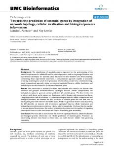
Fig. 2 The GC-dependency in real data and simulated data. The GC-dependency in (a, b, c) three real sequencing data from the 1000 Genome Project and in (d, e, f) three simulated data generated by pysim-sv . The x-axis is the GC-proportion in 10 Kb bins and the y-axis is the number of mapped reads in the bins. Note that the lower bands in the left and middle panel of (a, b, c) correspond to bins in chromosome X and the two individuals here are two males. The functions in (d, e, f) are f1 , f2 and f3 as presented in the GC-bias introduction section
The Author(s) BMC Bioinformatics 2017, 18(Suppl 3):53
Page 26 of 175
positions. Then, they are generated backwardly from the last position to the first first position.
to user specified proportions of these genomes. By default, ART [22] is used to generate HTS data.
Tumor aneuploidy simulation
GC bias introduction
Aneuploidy is the deviation of ploidy number from the normal ploidy number. It is very common in cancer genomes and is related with chromosomal instability [20]. Aneuploidy has important impact on tumor CNV detection since it often causes incorrect estimation of copy numbers. Pysim-sv allows generation of aneuploidy according to user-specified aneuploidy status (the copy number of each chromosome) of the simulated genome. Pysim-sv generates genomes with aneuploidy from normal diploid genomes and the resulting genomes provide the starting genomes for somatic SV simulation.
After the initial HTS data are generated, we further employ a biased subsampling method to introduce GCbiases. Specifically, Pysim-sv first calculates a subsampling probability for every read pair (or every read for single-end data). This subsampling probability depends on the local GC-content of the sequence from which the read pair is generated. We use the following procedure to introduce GC-biases. Given a read pair (R1 , R2 ), let (S1 , S2 ) (S1 < S2 ) be the positions in the simulated chromosome from which the read pair was sequenced. Note that these reads are Illunima platform type reads. Then, the sequence S from S1 to S2 + r in the simulated chromosome is the segment that generates the read pair (r is the read length). Let GCS be the GC proportion of this segment. Then, we will subsample this read pair (R1 , R2 ) with probability pS = f (GCS )/(1 + f (GCS )), where f is a user specified function. Specifically, Pysim-sv first generates a random number from the Bernoulli distribution with the success rate as the probability pS . Pysim-sv will or will not select this read pair depending on whether or not the random number is 1. Figure 2 show examples of GC-dependency in real sequencing data (top panel) and in simulated data by Pysim-sv (bottom panel). The GCdependency functions in Fig. 2d–f are chosen as f1 (x) =
Tumor genome heterogeneity and purity simulation
Tumor cell populations often contain many heterogeneous subclones. Pysim-sv simulates new subclones from a progenitor genome by randomly placing new somatic variations. The number of new subclones from the progenitor genome can be specified by users. Iterative application of this procedure can be used to simulate the clone evolution model [3] as well as the cancer stem cell model [21]. After a specified number of subclones are simulated, Pysim-sv then simulates HTS short reads from these tumor/normal genomes, and mixes these reads according
Table 1 The sensitivity and false discovery rate (FDR) of the different SNV detection algorithms with different simulation setups Purity
Subclone1
Subclone2
GC-bias Yes
Purity=1
1
0
No
Yes Purity=0.8
0.4
0.4
No
Yes Purity=0.5
0.4
0.1
No
Methods
Sensitivity
FDR
GATK
0.97679
1.13 × 10⁻⁴
Varscan
0.97892
2.36 × 10⁻³
GATK
0.97826
9.20 × 10⁻⁵
Varscan
0.98134
2.05 × 10⁻³
GATK
0.90253
1.93 × 10⁻³
Varscan
0.92501
5.36 × 10⁻³
GATK
0.90853
8.32 × 10⁻⁴
Varscan
0.93001
5.05 × 10⁻³
GATK
0.81253
1.09 × 10⁻²
Varscan
0.84501
5.34 × 10⁻²
GATK
0.81853
2.11 × 10⁻³
Varscan
0.85001
4.51 × 10⁻²
Note that the purity column represents the proportion of “tumor” cells in the simulated data. Subcolone1 and Subcolone2 columns represent the proportions of subcolone 1 and 2 in the simulated data, respectively. When purity is 1 and subclone1 is 1, it means that all data are from subclone1 and it essentially like a sequencing data from a normal genome
The Author(s) BMC Bioinformatics 2017, 18(Suppl 3):53
c 0.8 Sensitivity 0.4 0.6 0.2
M
G AS V−
ee rk at
pr o
er
0.0 1.0 Sensitivity 0.6 0.4 0.2
at rk
Br
G
M
AS
V−
lly
De
ee
pr
ce an kD ea
M
G
o
r
0.0 at rk
pr V− AS
ee
o
r ce an kD
lly
De
Br
ea
M
G
deletion inversion translocation
0.8
1.0 0.8 0.2 0.0 at rk
pr V− AS
ee
o
r ce an kD ea Br
lly
De
f
Sensitivity 0.4 0.6
0.8 Sensitivity 0.4 0.6 0.2 0.0
lly
De
Br ea kD an c
ee rk at M
G AS V−
lly
De
e
1.0
d
pr o
er
0.0 M
Br ea kD an c
lly
De
ee rk at
pr o G AS V−
Br ea kD an c
er
0.0
0.2
0.2
Sensitivity 0.4 0.6
Sensitivity 0.4 0.6
0.8
0.8
1.0
1.0
b
1.0
a
Page 27 of 175
purity=1
purity=0.8
purity=0.5
Fig. 3 The sensitivity of the four SV detection algorithms with different parameters. Deletions (black), inversion (grey) and translocations (white) are compared, individually. a, b, and c are the simulated data with GC-bias, and d, e, f are the simulated data without GC-bias. The purities are 1 (a, d), 0.8 (b, e) and 0.5 (c, f)
−8.89x3 −3.56x2 +9.13x−1.58, f2 (x) = −2.5(x−0.6)2 +1, and ⎧ x ≥ 0.4 ⎨ −2x + 1.8 4x − 0.6 0.2 ≤ x ≤ 0.4 f3 (x) = ⎩ 0.1 otherwise. Note that the GC-dependency functions of Fig. 2d–f are not chosen to be corresponding to GC-dependency of Fig. 2a–c. Pysim-sv is very flexible in generating GCbias and users can easily specify any GC-dependency functions.
Results and Discussions Based on the human reference genome (hg19), we simulated six genomes with three levels of purity (1, 0.5, and 0.8) and two levels of GC-dependency (with and without GC-bias). Each genome contains 100,000 SNVs and 200 SVs. We generated 30× 100 bp paired-end read data. We
used GATK [23] and Varscan [24] to detect SNVs in these simulated data, and used Delly [25], BreakDancer [6], GASV-Pro [26] and Meerkat [5] to detect SVs. As a comparison, we also ran these algorithms on a real data set NA12878 from the 1000 Genome Project. The NA12878 data was sequenced on the Illumina platform with a read length of 100 bp. The mean insert size is 320 bp with a standard deviation of 60 bp. The coverage of this data set is around 40×. Table 1 shows the sensitivity and false discovery rate (FDR) of GATK and Varscan on the six simulated data. We found that Varscan had a higher sensitivity and FDR rate than GATK. The sensitivities of GATK and Varscan tend to decrease and their FDR rates tend to increase when the purity decreases. Similarly, compared with no GC-bias data, their sensitivities are lower and their FDRs are higher when GC-bias is introduced. On the NA12878 data, by comparing with reported SNVs
Table 2 Overlaps of deletion predictions of the four SV detection algorithms with golden standard deletions in Mills el. al. 2011 Software Delly
Total reported deletion
Deletions in golden standard
Precision
1075
358/545
0.33
Recall rate 0.66
BreakDancer
779
328/545
0.42
0.60
Gasv-pro
1382
339/545
0.25
0.62
Meerkat
687
372/545
0.54
0.68
The Author(s) BMC Bioinformatics 2017, 18(Suppl 3):53
Page 28 of 175
a Log2 copy ratio
2
BIC-seq2 Detected CNVs
1 0
-1 -2 20
30 chromosome 22 (Mb)
40
20
30 chromosome 22 (Mb)
40
b Log2 copy ratio
2
Simulated True CNVs
1 0
-1 -2
Fig. 4 True CNVs in a simulated genome and detected by BIC-seq2. a Forty CNVs were introduced in the simulated genome and thirty-five copy number gains (red lines) and copy number losses (blue lines) were detected by BIC-Seq2. b True copy number gains (red lines) and copy number losses (blue lines) in the simulated genome
of this individual from the 1000 Genome Project, the sensitivities of GATK and Varscan were 96.8 and 96.3%, similar to their performances on the simulated data set with purity 1. The sensitivities of the SV detection algorithms are shown in Fig. 3. Compared with the SNV detection algorithms, the sensitivities of these algorithms are relatively low. All methods have sensitivities above 75%. Meerkat and Delly achieved higher sensitivity rates than BreakDancer and GASV-Pro because Meerkat and Delly used both discordant reads and split reads to detect SVs. As the purity decreases, we also observe that the sensitivities of the SV detection algorithms tend to decrease. For NA12878, we compared the SV calls from the four SV detection algorithms with the golden standard SV set
as reported in Mills et al. 2011 [1]. Since most of the reported SVs in Mills et al. 2011 are deletions, we only considered deletion predictions. The precision and recall rates of the four algorithms are calculated by comparing with the golden standard deletions (Table 2). The precisions of the four algorithms are relatively low, but this low level of precision might be due to the possibility that many true deletions are not included in the golden standard set. For CNV detection, we generated another simulation data containing 40 CNVs with their sizes ranging from 100 bp to 10 kb and their copy numbers ranging from 0 to 6. SNVs and Indels were also introduced to this genome by randomly sampling from the dbSNP database. We used Pysim-sv coupled with ART to generate 10× data of 100 bp paired-end reads with GC-bias. BIC-seq2 [13, 27]
Table 3 The running time (hour) and memory usage (Gb) for Pysim-sv simulations with different parameter settings Simulation set up Genome Simulationa
Read generationb
a
Time
Memory
One subclone with 100 SVs
0.98 h
9.1 Gb
One subclone with 200 SVs
1.34 h
9.9 Gb
One subclone with 300 SVs
1.73 h
11.6 Gb
Two subclones with 100 SVs
1.03 h
9.5 Gb
Three subclones with 100 SVs
1.28 h
10.2 Gb
Mixing reads from 2 subclones and 1 normal genome (392 M reads)
2.76 h
6.2 Gb
GC-bias Introduction (130 M reads)
4.10 h
2.5 GB
Time and memory usage for simulating subclone genomes and a normal genome b Time and memory usage for read generation by ART are not shown
The Author(s) BMC Bioinformatics 2017, 18(Suppl 3):53
was used to detect CNVs based on BWA [28] mapping. Among 40 CNVs, 35 were detected by BIC-Seq2 (Fig. 4). To test Pysim-sv speed, we used a diploid human genome(hg19) as reference and evaluated the computational efficiency with different parameter settings. We simulated 2.4 million SNVs which were randomly selected in dbSNP. We simulated 1–3 subclones with 100–300 SVs ranging from 1 to 10 kb. The test was performed on a 32-core sever with Intel Xeon 2.40 GHz CPU, running a Linux operating system. The running time and the memory usage of Pysim-sv were summarized in Table 3.
Page 29 of 175
Authors’ contributions YX implemented the package. YX and RX wrote the paper. YX and YL performed the analysis. All authors have read and approved the final manuscript. Competing interests The authors declare that they have no competing interests. Consent for publication Not applicable. Ethics approval and consent to participate Not applicable. Published: 14 March 2017
Conclusion In this paper, we present Pysim-sv to simulate HTS data for benchmarking SV detection algorithms. Pysim-sv can simulate a wide spectrum of germline and somatic variations and thus the simulated genomes are more similar to real genomes. Pysim-sv is the first HTS data simulation tool that can introduce the GC-bias in the simulated HTS data. These features make simulation data generated by Pysim-sv more similar to real HTS data. We believe that Pysim-sv is a useful toolkit for performance evaluation of SV detection and SNV detection algorithms based on HTS data.
Availability and requirements Project name: Pysim-sv Project home page: https://github.com/xyc0813/pysim/ Operating system(s): Windows,Unix-like (Linux, Mac OSX) Programming language: python(>=2.7) Any restrictions to use by non-academics: None Abbreviations CNV: Copy number variation; HTS: High throughput sequencing; NAHR: Non-allelic homologous recombination; NHR: Non-homologous recombination SVs: Structural variations; SNVs: Single nucleotide variations Acknowledgements We thank Prof. Qian Minping for advice and discussions during program development. Part of the analysis was performed on the Computing Platform of the Center for Life Science. Declarations This article has been published as part of BMC Bioinformatics Volume 18 Supplement 3, 2017. Selected articles from the 15th Asia Pacific Bioinformatics Conference (APBC 2017): bioinformatics. The full contents of the supplement are available online https://bmcbioinformatics.biomedcentral.com/articles/ supplements/volume-18-supplement-3. Funding The National Key Basic Research Project of China (2015CB856000); The National Natural Science Foundation of China (11471022, 71532001); Recruitment Program of Global Youth Experts of China; Funding for publication cost: the National Key Basic Research Project of China. Availability of data and materials The simulated data supporting the conclusions of this article was created using Pysim-sv which is available at https://github.com/xyc0813/pysim/.
References 1. Mills RE, Walter K, Stewart C, Handsaker RE, Chen K, Alkan C, Abyzov A, Yoon SC, Ye K, Cheetham RK, et al. Mapping copy number variation by population-scale genome sequencing. Nature. 2011;470(7332):59–65. 2. Sismani C, Koufaris C, Voskarides K. Copy number variation in human health, disease and evolution. In: Genomic Elements in Health, Disease and Evolution. New York: Springer; 2015. p. 129–54. 3. Ding L, Wendl MC, Koboldt DC, et al. Analysis of next generation genomic data in cancer: accomplishments and challenges. Hum Mol Genet. 2010;19(R2):188–96. 4. Stephens PJ, Greenman CD, Fu B, Yang F, Bignell GR, Mudie LJ, Pleasance ED, Lau KW, Beare D, Stebbings LA, et al. Massive genomic rearrangement acquired in a single catastrophic event during cancer development. Cell. 2011;144(1):27–40. 5. Yang L, Luquette LJ, Gehlenborg N, Xi R, Haseley PS, Hsieh CH, Zhang C, Ren X, Protopopov A, Chin L, et al. Diverse mechanisms of somatic structural variations in human cancer genomes. Cell. 2013;153(4):919–29. 6. Chen K, Wallis JW, McLellan MD, Larson DE, Kalicki JM, Pohl CS, McGrath SD, Wendl MC, Zhang Q, Locke DP, et al. BreakDancer: an algorithm for high-resolution mapping of genomic structural variation. Nat Methods. 2009;6(9):677–81. 7. Bartenhagen C, Dugas M. RSVSim: an R/Bioconductor package for the simulation of structural variations. Bioinformatics. 2013;29(13):1679–81. 8. Qin M, Liu B, Conroy JM, et al. SCNVSim: somatic copy number variation and structure variation simulator. BMC Bioinforma. 2015;16(1):1–6. 9. Mu JC, Mohiyuddin M, Li J, et al. VarSim: a high-fidelity simulation and validation framework for high-throughput genome sequencing with cancer applications. Bioinformatics. 2015;31(9):1469–71. 10. Yuan X, Zhang J, Yang L. IntSIM: An integrated simulator of next-generation sequencing data. IEEE Trans Biomed Eng. 2016;1–11. 11. Pattnaik S, Gupta S, Rao AA, Panda B. SinC: an accurate and fast error-model based simulator for snps, indels and cnvs coupled with a read generator for short-read sequence data. Bmc Bioinformatic. 2013;15(1):1–9. 12. Hu X, Yuan J, Shi Y, Lu J, Liu B, Li Z, Chen Y, Mu D, Zhang H, Li N. pIRS: Profile-based illumina pair-end reads simulator. Bioinformatics. 2012;28(11):1533–5. 13. Xi R, Lee S, Xia Y, et al. Copy number analysis of whole-genome data using BIC-Seq2 and its application to detection of cancer susceptibility variants. Nucleic Acids Res. 2016;44(13):6274–86. 14. Sherry ST, Ward MH, Kholodov M, Baker J, Phan L, Smigielski EM, Sirotkin K. dbSNP: the ncbi database of genetic variation. Nucleic Acids Res. 2001;29(1):308–11. 15. Bamford S, Dawson E, Forbes S, Clements J, Pettett R, Dogan A, Flanagan A, Teague J, Futreal PA, Stratton M, et al. The COSMIC (catalogue of somatic mutations in cancer) database and website. Br J Cancer. 2004;91(2):355–8. 16. Forbes SA, Bindal N, Bamford S, et al. COSMIC: mining complete cancer genomes in the catalogue of somatic mutations in cancer. Nucleic Acids Res. 2011;39(suppl_1):D945–D950. 17. Currall BB, Chiangmai C, Talkowski ME, Morton CC. Mechanisms for structural variation in the human genome. Curr Genet Med Rep. 2013;1(2):81–90. 18. Meyer LR, Zweig AS, Hinrichs AS, Karolchik D, Kuhn RM, Wong M, Sloan CA, Rosenbloom KR, Roe G, Rhead B, et al. The UCSC genome browser
The Author(s) BMC Bioinformatics 2017, 18(Suppl 3):53
19. 20. 21. 22. 23.
24.
25.
26.
27.
28.
Page 30 of 175
database: extensions and updates 2013. Nucleic Acids Res. 2013;41(D1): 64–9. Kumar D. Disorders of the genome architecture: a review. Genomic Med. 2008;2(3-4):69–76. Hassold T, Hunt P. To err (meiotically) is human: the genesis of human aneuploidy. Nat Rev Genet. 2001;2(4):280–91. Shackleton M, Quintana E, Fearon ER, Morrison SJ. Heterogeneity in cancer: cancer stem cells versus clonal evolution. Cell. 2009;138(5):822–9. Huang W, Li L, Myers JR, Marth GT. ART: a next-generation sequencing read simulator. Bioinformatics. 2012;28(4):593–4. McKenna A, Hanna M, Banks E, Sivachenko A, Cibulskis K, Kernytsky A, Garimella K, Altshuler D, Gabriel S, Daly M, et al. The genome analysis toolkit: a mapreduce framework for analyzing next-generation dna sequencing data. Genome Res. 2010;20(9):1297–303. Koboldt DC, Chen K, Wylie T, Larson DE, McLellan MD, Mardis ER, Weinstock GM, Wilson RK, Ding L. VarScan: variant detection in massively parallel sequencing of individual and pooled samples. Bioinformatics. 2009;25(17):2283–285. Rausch T, Zichner T, Schlattl A, Stütz AM, Benes V, Korbel JO. Delly: structural variant discovery by integrated paired-end and split-read analysis. Bioinformatics. 2012;28(18):333–9. Sindi SS, Onal S, Peng LC, Wu HT, Raphael BJ. An integrative probabilistic model for identification of structural variation in sequencing data. Genome Biol. 2012;13(3):22. Xi R, Hadjipanayis AG, Luquette LJ, Kim TM, Lee E, Zhang J, Johnson MD, Muzny DM, Wheeler DA, Gibbs RA, et al. Copy number variation detection in whole-genome sequencing data using the bayesian information criterion. Proc Natl Acad Sci. 2011;108(46):1128–36. Li H, Durbin R. Fast and accurate short read alignment with burrows–wheeler transform. Bioinformatics. 2009;25(14):1754–60.
Submit your next manuscript to BioMed Central and we will help you at every step: • We accept pre-submission inquiries • Our selector tool helps you to find the most relevant journal • We provide round the clock customer support • Convenient online submission • Thorough peer review • Inclusion in PubMed and all major indexing services • Maximum visibility for your research Submit your manuscript at www.biomedcentral.com/submit