[6] Pounds P., Mahony R., Hynes P. and Roberts J.,. Design of a Four-Rotor Aerial ... Conference, 2004. [8] How J.P., Bethke B., Frank A., Dale D. and Vian J.
QUADROTOR CONTROL BASED ON PARTIAL SENSOR DATA Laszlo Kis*
Bela Lantos*
*Departement of Control Engineering and Information Technology Budapest University of Technology and Economics ABSTRACT A miniature quadrotor helicopter is an underactuated nonlinear system. Usually several types of sensors are used to control it. This article focuses on the emergency situation, when only few sensors are available. These sensors are mainly the inertial ones. Certainly, these sensors are not enough for normal manoeuvring, but the controlled system should be able for horizontal stabilization and safe landing. Two types of control are presented. The first is a casual LQ state feedback. The disadvantage of this type of control in real environment is shown. The second control algorithm is an H∞ control method. The control design starts from a very simple linear model. The parameter measurement of the linear system is shown. The goal of this article is to handle the uncertainty in the behaviour of the real system. Keywords: Quadrotor helicopter, state estimation, helicopter control, robust control
1 INTRODUCTION Unmanned aerial vehicles are important types of autonomous vehicles. Helicopters have the advantage that they can move in six degree of freedom with low speed. Mechanically, a robust type is the quadrotor design. This type has been forgotten for a long time, because in small size, they have fast unstable behaviour. Nowadays, there are controllers and sensors, which are fast enough to stabilize a quadrotor helicopter. 1.1 RELATED WORK In the last few years many research group started to work with quadrotors. Most of them concentrate on a specific field of quadrotor design. For example [1], [2], [3], [4] describe different types of control algorithms. Usually these solutions are tested on a skeleton of a quadrotor helicopter. Others describe the electrical and mechanical solutions of their work. In these cases a complex helicopter is built [5], [6]. Some researchers designed a fully autonomous system, like the STARMAC and RAVEN platform [7], [8]. Quadrotor helicopters appeared in commerce, for example Draganfly and Microdrone products. These units are human controlled, but have built in function for stabilization or position hold. Contact author: Laszlo Kis1, Bela Lantos1 1
Departement of Control Engineering and Information Technology, Budapest University of Technology and
Economics, H-1117 Budapest Magyar Tudosok krt. 2. {lkis,lantos}@iit.bme.hu
1.2 RECENT PROJECT Our project started in 2006, in cooperation with the Department of Control Engineering and Information Technology in the Budapest University of Technology and Economics and the System and Control Lab of the Computer and Automation Research Institute of the Hungarian Academy of Sciences. The main goal of the project is to design and build an autonomous indoor quadrotor helicopter. In this project a vision system and inertial measurements system are used as sensory system. The control and state estimation algorithms of the normal usage are described in [9]. This article focuses on the situation, when some of the sensors are unreachable. This situation can happen for many reasons. For example the vision system cannot estimate the position of the helicopter because of occlusion. Or the radio channel can be too noisy between the vision system and the helicopter. In these situations the only sensors which can be used are the inertial ones. They can produce only relative information, therefore they can be used only for a short time. The types of manoeuvres are also limited. In these emergency cases, the main object is to hold the helicopter in horizontal orientation to prevent falling. A second objective can be the vertical landing, if the batteries are low. Solutions in this article can also be used in outdoor situations, where the absolute position and orientation sensing comes from the GPS. In these cases the reliability of the GPS can vary during time. After introduction, the used helicopter model is described in Section 2. Section 3 shows how the parameters were measured. Section 4 introduces the problems and solutions of state estimation. Section 5 describes the control design in normal operation. Section 6 presents the electrical components of the helicopter. Section 7 gives some hints how to operate in emergency situations. In Section 8 a basic LQ feedback result is presented. Finally in Section 9 an H∞ control is shown, which is robust against the model uncertainty. 2 THE HELICOPTER MODEL The graph of the coordinate systems of the helicopter can be seen in Figure 1. KW is the world frame and K H is the frame of the helicopter. K S ,0 is the original frame of the inertial measurement unit (IMU). This frame is rotated during the calibration method of the IMU to K S . The transformation between K H and K S is determined by the mechanics of the helicopter. Frames K C and K virt are used by the vision system described in [9].
Figure 1 Graph of the frames. The schematic physical principle of the helicopter is shown in Figure 2.
Figure 2 Forces of the quadrotor. The lift force of one propeller can be calculated according to: (1) F = Ω 2b where Ω is the revolution of the propeller and b is a propeller constant. Let l be the distance between the origin of helicopter's frame and the propeller's axis. Then the torques and lift force can be calculated: (2) τ x = (Ω 4 2 − Ω 2 2 )bl
τ y = (Ω 3 2 − Ω1 2 )bl
(3)
τ x = (Ω 2 2 − Ω12 + Ω 4 2 − Ω 3 2 )d
(4)
4
U =
∑ bΩ
2 i
(5)
i =1
where d is an other propeller constant. 2.1 MOTOR MODEL The dynamics of the motors should be considered during the modeling process. In our case the motor revolution is controlled by a low-level PI controller, and the closed loop behavior can be approximated with a first order system: 1 & Ω (Ω desired − Ω real ) (6) real = Tm where Tm is the motor time constant. In the followings the indices r and d will refer to real and desired value. Based on (6) and (2)-(5) the dynamic of the real torques and lift forces can be developed as a second order system, like: (7) τ d = Tm 2τ&&r + 2Tmτ&r + τ r For an easier control synthesis (7) will be approximated with a first order system: 1 τ&r = (τ d − τ r ) (8) 2Tm
This approximation can be done, if Tm is small, in our model its value is 0.1s. 2.2 ORIENTATION MODEL Based on the Newtonian law the linear dynamic model for the orientation can be described as T
τ x , r τ y ,r τ z ,r T (9) ϕ&& ϑ&& ψ&& = Θx Θy Θz where Θ is the inertia around the axes of the coordinate system. The equations are valid in the frame of the helicopter. These equations remain acceptable in the world frame, if the orientation of the helicopter remains horizontal. Therefore these can be considered as a linearized model around η = 0 , where η is the 3D Euler(RPY) orientation of the helicopter relative to world frame. In this dynamic model, the effect of the aerodynamic friction and the gyroscopic effect considered to be negligible. The aerodynamic friction is in linear connection with η& which is approximated with zero. The
(
)
measured with the fixation of all the six degree of freedom, except the rotation around the vertical axis. The torque around the axis should be measured for several rotor velocities and can be approximated by a parabola. In our measurement it is one order less than b. The inertia matrix can be determined with a torsion pendulum. The scheme of the pendulum can be seen in Figure 3.
gyroscopic effect is a function of the rotor inertia Θ r , this can be ignored, because the mass of each rotor is 0.4% of the full mass of the helicopter and this value is also in connection with the difference between the rotor’s revolution, which is around zero in a horizontal orientation.
Figure 3 Torsion pendulum. Inertia matrix is approximated as a diagonal one based on the symmetric shape of the helicopter. The inertia around one axis can be determined by the following formula: 2 T mgr 2 Θ= 0 2 (13) 4π l pend
2.3 POSITION MODEL Based on also the Newtonian law the position states are in the following form: (C S C + Sϕ Sψ ) &x&W = ϕ ϑ ψ (10) Ur m (C S S − Sϑ Cψ ) &y&W = ϕ ϑ ψ (11) Ur m C C &z&W = − g + ϕ ϑ U r (12) m where C• and S • refers to cosine and sine and g is the gravity acceleration.
where l pend is the length of the two torsion thread and r is
3 PARAMETER MEASUREMENT The unknown parameters are the b and d parameters of the propellers and the l and Θ parameters of the helicopter. The parameter l is the simplest, because this distance can be measured even with a measuring tape. In the case of our helicopter its value is 25 cm. The parameter b was determined by using lift force measurement. Lift force was measured in different rotor velocities and a parabola was fitted by using LS method. In our case the value of b is 1.4525 ⋅ 10 −5 Ns 2 . The d parameter is in connection with the torque around the vertical axis. Even if this value is in connection with l, it is easier to handle as a standalone parameter. It can be
the half distance between the threads. m is the mass of the helicopter and g is the gravity constant. T0 is the period time of the pendulum. This value was measured with a time-stamped camera. 4 STATE ESTIMATION For control algorithms, position and orientation information is needed. Moreover a sensor fusion between the IMU and the vision system should be performed. These problems are solved with extended Kalman filters. In first stage the orientation is estimated. Then based on orientation information the position is estimated. 4.1 ORIENTATION ESTIMATION For orientation estimation the sensor model is the following: ω S = ω S ,real + ω S ,b + ωS ,n (14) ω H ,real = Asω s − Asω s ,b + As ω S ,n (15) where As is the rotation part of Ts and indices b and n refer to bias and noise, respectively. The transformation between ω H and η& is
1 Sϕ Tϑ F = 0 Cϑ 0 Sϕ / Cϑ
Cϕ Tϑ − Sϕ Cϕ / Cϑ Then the model used for Kalman filter is η& = FAsω s − FAs ωs ,b + FAsω S ,n
ω& S ,b = ω S ,b ,n
(17)
The control algorithms are based on the continuous state space model (9)-(12). Controllers are implemented in discrete time, hence the model was transformed with first order Euler approximation. The Linear-Quadratic design minimizes the following error statement:
(18)
J=
(16)
ηv = η + ηn where
η
(19) is the orientation information from the vision
v
system. With Euler approximation for state x = (η , ω S ,b )T , u = ω S and y = η v , a discrete time system can be formulated: xk +1 = f ( xk , u k , wk ) (20) y k = g ( xk , z k ) (21) where w and z are state and measurement noises. With the following definition: R w,k = E[ wk wTk ], R z ,k = E[ z k z Tk ] (22) ∂f ( xˆ k , u k ,0) ∂f ( xˆ k , u k ,0) , Bw,k = ∂x ∂w ∂g ( x k +1 ,0) ∂g ( x k +1 ,0) C k +1 = , C z ,k +1 = ∂x ∂z The extended Kalman filter has the form: xk = f ( xˆ k −1 , u k −1 ,0) Ak =
Mk = Sk =
Ak −1Σ k −1 AkT−1
Ck M k CkT
+
Bv,k −1 Rv,k −1 BvT,k −1
+ C z ,k R z ,k C zT,k
M k CkT S k−1
Gk = xˆ k = xk + Gk ( y k − g ( xk ,0))
+ u Tk Ru k )
(35)
k =0
where Q and R are positive definite matrices. The weight matrix of the state vector is Q. The goal for the control is the output converges to the desired value. Therefore the highest value in Q should correspond to the output state. With the R matrix the speed of the control can be set. On the other hand a faster control means higher steps in actuator signals. A reliable compromise between Q and R should be found. The pure linear altitude subsystem is: T
(24)
The difference between (36) and (12) is the − g offset in
(25) (26) (27) (28) (29)
(31)
a& S ,b = a S ,b ,n
(32)
p& = Aη v + v p ,n
(33)
(34) where a, v refers to acceleration and velocity in K H , p is the position in KW , ε is the angular acceleration (obtained with the numeric derivation of ω ), ρ is the position part of Ts and Aη is the Euler (RPY) rotation pm = p + pn
based on the angles η . From this system an extended Kalman filter can be formulated similarly to the orientation case. 5 NORMAL CONTROL (ALTITUDE)
T k Qx k
(23)
Σk = (30) In the case when there is no new information from the vision system, in (29) simply xˆ k = x k to be applied.
− ε × ρ − ω × (ω × ρ ) + Aη −1 g
∑ (x
C C d (z&W zW U r )T = ϕ ϑ U r z&W 1 (U d − U r ) (36) dt 2Tm m
M k − Gk S k GkT
4.2 POSITION ESTIMATION The model for position estimation is the following: v& = −ω × v + AS (aS − a S ,b + a S ,n )
∞
zW . The LQ feedback can be designed to (36) and in the control g should be added to U d . The behavior of the real control can be seen in Figure4. During the normal operation the helicopter can hold its altitude. In this period an average U d value can be obtained, which will be useful in emergency control. The control for the other subsystems can be designed similarly. 6 REAL TIME SOLUTION The scheme of the realization of the helicopter can be seen in Figure 5. The main processing unit of the helicopter is a Freescale MPC555 microcomputer equipped with two CAN buses. The first one is the dedicated bus between the motor controllers and the MPC555. It is necessary to maintain a reliable and fast communication channel for the actuator signals. The second CAN bus is for any other communication. The CAN bus is a priority based communication interface. The most important data on the CAN bus are the sensor signals.
7 EMERGENCY CONSIDERATION
Figure 4 Result of the altitude control
Figure 5 Realization of the helicopter The helicopter has two types of sensory systems. The first one is an mNAV100CA inertial measurement unit which is on board of the helicopter. On CAN bus the information from the angular velocity and acceleration sensors are propagated. The second sensory system is a visual feedback from an external vision system, which is able to calculate the position and the orientation of the helicopter in the world frame around 20 to 30 sample per second. It runs on a host PC and data are sent by an RF Zigbee communication interface. The inertial information has the highest priority on the CAN channel and the vision information has the second highest. Unfortunately both the IMU and the RF module have no CAN interfaces. Therefore the packages should be translated to the CAN format using Atmel AT90CAN128 microcontrollers. The vision system has an active marker based solution. These markers are LEDs. For the efficiency of the vision unit the colours of the LEDs need to be different. To reach this requirement, RGB LEDs are used. It is rewarding, at least in the prototyping period, if the colours can be changed by software. Therefore each LED is controlled by its own individual controller.
In the case of the real time test of this paper, only the angular velocity sensors of the IMU were used in order to emulate emergency situation. To use the measured data a calibration method should be performed. This is described in [9]. The calibration method gives a usable result in the case of extended Kalman filters. However in emergency situation the calculation method of orientation is much more simple, only a numeric integration of the angular velocity data is used . During the first tests it seemed that the bias is rapidly varying during the flight. This is because of the generated air flow, which changes the temperature of the sensors. Fortunately there is a thermistor built in each angular velocity sensor chip. This information can be used to produce more accurate results. The temperature dependence can be measured during the offline calibration, but a varying temperature environment is needed. It is not a complicated condition, because after switch on the system, the temperature of the sensors starts to increase. This change is enough for the calibration. During the offline calibration the sensors are in stationary position, hence the measured angular velocity is only the biases. Combining with temperature measurement, a temperature-bias characteristic is given, which is approximated with a linear dependency. Then for an other measurement the bias were calculated based on the previous characteristic. The results are in the Figure 6.
Figure 6 Measured and temperature based calculated bias of an angular velocity component The corrections of the measurements are done by the MPC555 microcomputer. This unit solves also the integration of the angular velocity. In the case of angular velocity the component based integration leads to a false result. For proper result the Rodriguez-formula is used. In this case the axis of the rotation is the axis of the measured three dimensional angular velocity vector, and the angle of the rotation is the magnitude of the angular velocity vector multiplied by the sampling time.
tk =
(ϕ& k , ϑ&k ,ψ& k )T 2
2
ϕ& k + ϑ&k + ψ& k
2
α k = TS ϕ& k 2 + ϑ&k 2 + ψ& k 2
(37) (38)
where TS is the sensor sampling time, in this case 0.01s . The starting rotation matrix is the unit matrix. In each sampling period the actual rotation matrix should be multiplied with the Rodriguez rotation ( R R ): R R, k = Cα k ⋅ I + (1 − Cα k )[t k o t k ] + Sα k [t k ×] (39) Rk +1 = R R,k Rk
(40) where I is the unitary matrix and Rk describes the actual rotation. The (ϕ , ϑ ,ψ ) orientation angle can be calculated by the solution of the inverse Euler (RPY) problem. Figure 7 shows, how the error accumulates during the orientation calculation process. In the situation the sensors stood in stationary orientation, therefore the expected value is zero.
The state vector xk in (35) contains the values of angular velocity and orientation. In this case the main goal is to stabilize the orientation, therefore the weight of the orientation was set two order higher than the ones of the angular velocity. 8.1 SIMULATIONS The results of the simulation can be seen in Figure 8. The simulation was also done with a more complex nonlinear model, based on [1], but around horizontal orientation the two models are almost equivalent. During simulation the sensor noise is considered. 8.2 REAL FLIGHT The results of a real flight can be seen in Figure 9. This contains a vertical takeoff and landing. The main difference between the simulation and the real test is that in real situation the average of the orientation is not zero. This is because of the inadequate modelling of the real helicopter. Many source of this difference can be found. For example, the mass of the helicopter cannot be concentrated to the origin of the helicopter frame. Or the small differences between the propellers and motors can cause that the value b in the model differs from those of the motors. One solution for this problem can be the introduction of four different b parameters and the identification of them. In practice it is hard, because a complex identification process is needed after every change of the helicopter components.
Figure 7 Orientation estimation in stationary state
Figure 9 Orientation control with LQ (real test) 9 H∞ STABILIZATION Figure 8 Orientation stabilization with LQ control (simulation) 8 LQ STATE FEEDBACK (ORIENTATION) In the following chapters only the emergency control is discussed.
Another solution for the previous problem can be if the model stays as before, but the control removes the orientation error. This can be solved by using integrator in the controller. Let the continuous case be investigated. The classical solution [10] is to extend the state space system with an augmented state vector:
∫
x I = y dt
(41)
Then the augmented state space system is: d x A 0 x B = + u dt x I C 0 xi 0
(42)
y C 0 x = (43) x I 0 I x I The previous LQ design method could be used to this system. However, here a more robust H∞ control design is presented. The ∆ − P − K structure of the H∞ synthesis can be seen in Figure 10. [11]
Figure 10 Structure of H∞ synthesis The weights Wu and W p refers to model uncertainty and performance, respectively. Weights are set in the way, that in high frequency the uncertainty can be high, and in low frequency the stabilization of y should be fast. The resulted K (s ) controller is converted to discrete time with step response equivalence. 9.1 SIMULATION The result of the stabilization can be seen in Figure11. In this case the sensor noise is also simulated. It should be noted, that this type of H∞ design doesn’t remove the whole orientation error, but the remaining error can be set with the weights of the performance outputs to a very small value.
9.2 REAL FLIGHT The result of a complex real take off, flight and landing is shown in Figure 12. The orientation gets much closer to zero than in the case of LQ control. A small error still remains, as it was expected after the simulation. It should be noted, that the orientation starts from a zero value, but after landing the orientation has a small amount of offset. The bias of the angular velocity sensor is compensated by the temperature, but other components can also change the bias. The remaining error is caused by the integration of the remaining bias.
Figure 12 H∞ stabilization (real test) 10 CONCLUSION In this paper a quadrotor helicopter control is presented for the case where only the inertial sensors are reliable. In our case this situation can happen if the vision system cannot compute the orientation and position of the helicopter. It can be considered an emergency situation, in which the first requirement is to stabilize the orientation of the helicopter. The presented control can also be used as a startup controller to execute a take off and make a horizontal stabilization. During this period the controller can handle and estimate the uncertainty behaviour, which can be useful in controlling complex manoeuvres. It is also shown, why a simple state feedback controller is not sufficient for quadrotor control. In the emergency control system only the angular velocity sensor is used. A temperature compensation method is used for improving angular velocity integration. 10.1 FUTURE WORK The goal of our project is to establish a quadrotor system consisting three individual helicopters, which are able to flight in formation. During this way, the next step is to combine the emergency controller presented in this paper with a more complex one [12]. Then the system will be able to fly through a preprogrammed path and perform safe landing also in emergency situation.
Figure 11 H∞ stabilization (simulation)
The second future plan is to combine a quadrotor helicopter with a differential GPS system and perform outdoor operations. ACKNOWLEDGMENT This work is connected to the scientific program of the "Development of quality-oriented and harmonized R+D+I strategy and functional model at BME" project. This project is supported by the New Hungary Development Plan (Project ID: TÁMOP-4.2.1/B-09/1/KMR-2010-0002) The research was also supported by the Hungarian National Research Program under grant No. OTKA K 71762. REFERENCES [1] Bouabdallah S., Murrieri P. and Siegwart R., Design and Control of an Indoor Micro Quadrotor. International Conference on Robotics and Automation, New Orleans, USA, 2004. [2] Madani T., Benallegue A., Control of a Quadrotor Mini-Helicopter via Full State Backstepping Technique. IEEE Conference on Decision and Control, San Diego, USA, 2006. [3] Das A., Lewis F., Subbarao K., Backstepping Approach for Controlling a Quadrotor Using Lagrange Form Dynamics. Journal of Intelligent and Robotic Systems, September 2009, Vol. 56, pp. 127151. [4] Voos H., Nonlinear control of a quadrotor microUAV using feedback-linearization. IEEE International Conference on Mechatronics, Malaga, 2009 [5] Hanford S. D., Long L. N. and Horn J. F., A Small Semi Autonomous Rotary-Wing Unmanned Air Vehicle (UAV). American Institute of Aeronautics and Astronautics, Infotech@Aerospace Conference, 2005. Paper No. 2005-7077 [6] Pounds P., Mahony R., Hynes P. and Roberts J., Design of a Four-Rotor Aerial Robot. Australasian Conference on Robotics and Automation, 2002. [7] Hoffmann G., Rajnarayan D. G., Waslander S. L., Dostal D., Jang J. S. and Tomlin C. J., The Stanford Testbed of Autonomous Rotorcraft for Multi Agent Control (Starmac). Digital Avionics Systems Conference, 2004. [8] How J.P., Bethke B., Frank A., Dale D. and Vian J. Real-time indoor autonomous vehicle test environment, IEEE Control Systems Magazine, 28(2) pp. 51-64. ISSN: 0272-1708, 2008. [9] Kis L., Prohaszka Z. and Regula G., Calibration and Testing Issues of the Vision, Inertial Measurement and Control System of an Autonomous Indoor Quadrotor Helicopter, International Workshop on Robotics in Alpe-Adria-Danube Region, Ancona, Italy, 2008.
[10] Khuo B. C., Golnaraghi F., Automatic Control Systems, Wiley, ISBN 0-471-13476-7 [11] Zhou K., Doyle J.C., Glover K., Robust and Optimal Control, Prentice Hall, Englewood Cliffs, New Jersey 07632 [12] Kis L., Regula G. and Lantos B., Design and Hardware-in-the-Loop Test of the Embedded Control System of an Indoor Quadrotor Helicopter, Workshop on Intelligent Solutions in Embedded Systems, Regensburg, Germany, 2008.