Quantum state reduction for universal measurement based computation

Quantum state reduction for universal measurement based computation Xie Chen,1 Runyao Duan,2, 3 Zhengfeng Ji,4, 5 and Bei Zeng6, 7

arXiv:1002.1567v1 [quant-ph] 8 Feb 2010

1

Department of Physics, Massachusetts Institute of Technology, Cambridge, Massachusetts, USA 2 Centre for Quantum Computation and Intelligent Systems, Faculty of Engineering and Information Technology, University of Technology, Sydney, NSW, Australia 3 Department of Computer Science and Technology, Tsinghua National Laboratory for Information Science and Technology, Tsinghua University, Beijing, China 4 Perimeter Institute for Theoretical Physics, Waterloo, Ontario, Canada 5 State Key Laboratory of Computer Science, Institute of Software, Chinese Academy of Sciences, Beijing, China 6 Institute for Quantum Computing, University of Waterloo, Waterloo, Ontario, Canada 7 Department of Combinatorics and Optimization, University of Waterloo, Waterloo, Ontario, Canada (Dated: Feb 8, 2010) Measurement based quantum computation (MBQC), which requires only single particle measurements on a universal resource state to achieve the full power of quantum computing, has been recognized as one of the most promising models for the physical realization of quantum computers. Despite considerable progress in the last decade, it remains a great challenge to search for new universal resource states with naturally occurring Hamiltonians, and to better understand the entanglement structure of these kinds of states. Here we show that most of the resource states currently known can be reduced to the cluster state, the first known universal resource state, via adaptive local measurements at a constant cost. This new quantum state reduction scheme provides simpler proofs of universality of resource states and opens up plenty of space to the search of new resource states, including an example based on the one-parameter deformation of the AKLT state studied in [Commun. Math. Phys. 144, 443 (1992)] by M. Fannes et al. about twenty years ago. PACS numbers: 03.67.Lx, 03.67.Pp

Measurement based quantum computation (MBQC) [1], an interesting computation model that incorporates peculiar aspects in quantum mechanics like entanglement and measurement, achieves the full power of quantum computing by adaptive local measurements on a resource state. The first MBQC scheme, also known as the one-way quantum computation, employs the now well-known cluster state [2]. The highly entangled feature of the cluster state indicates that high entanglement is a key requirement for universality in MBQC. Although this is true in some sense [3, 4], it is also clear now that too much entanglement could also undermine universality [5, 6]. In other words, the entanglement should be manageable in a structured way. As shown in the recent breakthrough made by D. Gross et al. in Refs. [7, 8], the matrix product state (MPS) formalism [9, 10] or, in higher spacial dimensions, the computational tensor networks (CTN) [8, 11, 12] provides such an infrastructure for manipulating the entanglement and brings a new scheme of MBQC called the correlation space quantum computation. In this framework, a lot of new resource states beyond the cluster state are proposed. Most of the new resource states have different properties from the cluster state concerning, for example, local entropy, the two-point correlation function and the locality of the Hamiltonians of which they are unique ground states. Especially, some of the new resources are unique ground states of more practical Hamiltonians [13, 14], thereby overcoming the major flaw of the cluster state of not being a unique ground state of any two-body nearest-neighbour gapped Hamiltonian [15]. Here, we introduce the concept of quantum state reduction for MBQC and the motivation is twofold. First of all,

state reduction serves as a tool for revealing the entanglement structure of universal resource states [16, 17]. Similar to the common technique to study entanglement by considering local transformations [18–20], quantum state reduction is also a type of local transformation tailored to meet the nature of MBQC. We find out that almost all known resource states can be locally transformed to a cluster state via quantum state reduction, indicating that these resource states possess similar entanglement structure as the cluster state. Compared to the attempt made in Ref. [21], where it was shown that almost all these resource states are “universal state preparators”, quantum state reduction is a more direct approach and most notably more respectful for the geometry of the resource. Secondly, although the application of the MPS/CTN formalism in the theory of MBQC is elegant and fruitful, the routine for analyzing the universality of a resource state remains a complicated procedure, including the initialization, embedding of universal rotations, the readout, and compensation for the randomness. The quantum state reduction approach largely simplifies the analysis. For example, the universality of AKLT state [22, 23] is now cleanly summarized in Fig. 2. The simplicity also enables us to find new resource states, giving the universality of two deformations of AKLT state almost for free. To be more precise, our state reduction is a transformation from one resource state to some other universal target state (usually the cluster state) using local measurement and adaptive classical control. This transformation is named reduction as it resembles the reduction in complexity theory—as long as |Ψi is reducible to |Φi, it is in principle no harder to construct MBQC schemes for |Ψi than for |Φi. It is important to note

2 that, although the reduction is a random procedure, it always succeeds in obtaining a target state. Possibly, the resulting state may consist much smaller number of particles than the state before reduction. However, the cost or efficiency of the reduction, measured by the diminution in the number of particles, is always expected to be a constant. Matrix product states.—Following the notion in Refs. [7, 8], a matrix product state |Ψn i of n particles has the following form |Ψn i =

d−1 X

hR|A[xn ] · · · A[x1 ]|Li|x1 · · · xn i.

(1)

x1 ,··· ,xn =0

The physical dimension of each site is d, while the bond dimension of the state defined by the size of the matrices is δ. In general, one may consider an MPS where the defining matrices are site-dependent. The defining matrices are usually far more important than the boundary conditions hR|, |Li and sometimes we will use only the d-tuple (A[0], . . . , A[d − 1]) to specify an MPS. We will ignore the effect of a local change of basis on the physical space. For example, a state may be said to have some MPS representation even though this is only true up to some local unitary operations. Also for simplicity, A[x]’s will be given up to Psome normalization constant, which can be figured out from x A[x]† A[x] = I shown in Ref. [9]. A lot of states of particular interest in quantum information are indeed matrix product states of small bond dimension. The cluster state of one spacial dimension (i.e. a chain, or a 1-D cluster state), for example, is an MPS with defining matrices (H, HZ), where H, X, Y, Z are used to denote the Hadamard and Pauli matrices respectively. The GHZ state can be represented by (I, Z) up to local rotations. Another intriguing example is the AKLT state [22, 23] first studied in condensed matter theory. It will be shown in the next section that it has a simple MPS representation (I, X, Z). The correlation space quantum computation employs the structure of MPS as in Eq. (1). It starts with the initial state |Li of the so called correlation space, measures the physical spaces sequentially and thereby processes the correlation space, and finally reads out the information stored in the correlation space. Several new universal resources for MBQC were introduced in Refs. [7, 8] including a modified AKLT state with defining matrices (H, X, Y ). Later, the original AKLT state is also shown to be universal for MBQC [13]. Recently, the concept of quantum wires is defined and fully characterized in Ref. [24], which essentially gives the explicit condition for an MPS with d = δ = 2 to be a universal resource. There are two normal forms of the matrices for quantum wires. One is the “byproduct normal form” √ √ (2) A[0] = W/ 2, A[1] = W S(φ)/ 2, and the other is the “biased normal form” [25] A[0] = sin γ W ′ , A[1] = cos γ W ′ Z,

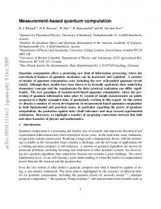
There is a higher spacial dimensional generalization of MPS, known by the names of the computational tensor networks [8], or the projected entangled pair state (PEPS) [11, 12]. Due to limitations of space, we refer the readers to the references above for details. The tabular form.—For the convenience of later discussions, we introduce a tabular form of MPS. In the tabular form, one writes the defining matrices of a block of sites explicitly in a table, where each column consists the d matrices of a corresponding site. The physical indexes determine a selection of one matrix from each column, whose product gives the correct amplitude together with the boundary conditions hR| and |Li. From the definition in Eq. (1) and the properties of MPS [9], we have 1) For any two neighboring columns, multiplication of M to the right of all matrices in the left column and M −1 to the left of all matrices in the right column simultaneously does not change the state; 2) A unitary transformation in the physical space corresponds to linear combinations of entries in the column with coefficients of the unitary; 3) Measurement in the computational basis corresponds to the deletion of column entries not consistent with the measured outcome; and 4) Columns of single entry can be removed by absorbing them to a neighboring column. We will use binary relations =, ≃ and ≺ to represent equality, local unitary equivalence and quantum state reduction respectively. As an example, Table 1 of Fig. 1 consists of a block of two sites of the AKLT states which will be discussed in the next section and it equals Table 2 by Property 1) of the tabular form. Reduction of the AKLT state.—The AKLT state [22, 23], named after Affleck, Kennedy, Lieb, and Tasaki, has become one of the prototypical states of spin systems. It also gives an excellent example for quantum state reduction. As the origin of matrix product states, the AKLT state bears a simple MPS representation with √ √ (4) A[0] = Z, A[1] = 2 |0ih1|, A[2] = 2 |1ih0|. Up to a local unitary operation, the matrices of the AKLT state can also be chosen as (X, Y, Z). In fact, any three different matrices of the identity and the Pauli matrices will work. For example, Fig. 1 presents the proof that (I, X, Z) also stands for the AKLT state. In this figure, Table 2 is obtained by adding the Y ’s with blue color, and hence represents the same state as Table 1 by Property 1) of tabular form; Table 2 and 3 describe two states that are equivalent under local unitary operations by Property 2). 1 X X Y Y Z Z

=

2 XY YX YY YY ZY YZ

≃

3 Z Z I I X X

FIG. 1. AKLT as (I, X, Z)

(3)

where W, W ′ are rotations along axes in the X-Z plane of the Bloch sphere and S(φ) = exp(−iφZ/2).

We now show the reduction from the AKLT state to the 1-D cluster state. It is convenient to start with the (I, X, Z) form.

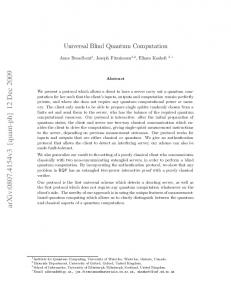
3 Two different measurements N1 and N2 will be used alternatively, where N1 measures {|0i, |1i} versus |2i, and N2 measures {|0i, |2i} versus |1i. That is, each measurement consists a two dimensional and a one dimensional projectors. The measurements are called success (failure) if the outcome corresponds to the two (one) dimensional subspaces. We measure the two measurements sequentially along the AKLT chain and switch the measurement we use only when the previous one succeeds. This simple procedure is called the alternating measurement scheme. Table 1 in Fig. 2 denotes a possible result after the alternating measurements on the AKLT state. More specifically, one first measures N1 and succeeds. Next, the measurement N2 is used. It results in the single dimensional space |1i once, and succeeds subsequently, and so on. After renaming the physical indexes and absorbing the X and Z in red color to their previous columns, we have Table 2 in Fig. 2 by Property 4) and 2). This is actually already a 1-D cluster state by the second line of reasoning in Fig. 2. 1 I I I I X X X Z Z Z

3 I I X Z

=

≃

4 IH HI XH HZ

2 I I I I X Z X Z

=

5 H H HZ HZ

FIG. 2. AKLT reduced to 1-D cluster

Families of universal states of AKLT type.— The simplicity of the above analysis enables us to generalize the same approach to a larger family of AKLT type of states. Notice that the key property that validates the first line of Fig. 2 is simply X 2 = Z 2 = I and the key to the second line is that H 2 = I and XH = HZ. We now choose two unitary matrices A and B such that A2 = B 2 = I, where A, B correspond to π-rotations along na and nb on the Bloch sphere respectively. Let C ∝ A + B be the π-rotation along na + nb . We will have C 2 = I and AC = CB. Therefore, we can prove the following reduction similarly (I, A, B) ≺ (C, CB).

(5)

Employing the gauge freedom of the representation of MPS, one can always choose B to be Z and C to be sin θX +cos θZ, making (C, CB) a quantum wire in the normal form of Eq. (2). Note that the 1-D AKLT state is a special case where θ = π/4 and that the error group hC, Bi is isomorphic to the dihedral group for infinitely many θ’s. With techniques of Ref. [9], one can check that the new AKLT type resource is always unique ground state of a nearest-neighbor, frustrationfree Hamiltonian. In Ref. [10], Fannes, Nachtergaele and Werner considered another one-parameter deformation of the AKLT model

whose ground state is an MPS with A[0] = sin θZ, A[1] = cos θ|0ih1|, A[2] = cos θ|1ih0|. We will show the universality of these states also by reduction. First, the defining matrices can be chosen as √ √
sin θZ, cos θX/ 2, cos θY / 2 , ˆ up to local unitary √ transformation. Let θ be the angle that satisfies tan θˆ = 2 tan θ. The defining matrices can be simpliˆ cos θX, ˆ cos θZ), ˆ fied to (sin θI, in the same way as in Fig. 1. Using a similar alternating measurement scheme in Fig. 2, this ˆ cos θHZ), ˆ is further reducible to (sin θH, a universal state in the biased normal form of Eq. (3). One caveat is that, in this case, we cannot simply absorb the X and Z in red color in Fig. 2 to neighboring sites because of the bias. But one can always measure the computational basis in several neighboring sites and cancel their effects by a random walk on the Pauli group. Reduction of quantum wires to cluster states.—We now discuss the reduction of universal quantum wires to the cluster state. The special case of (W, W Z) is much easier to deal with. To transform it into (H, HZ), one can simply implement HW † in the correlation space using the sites beforehand. In the general case of (W, W S(φ)), however, one cannot succeed using projective measurement only—the local entropy determined by φ [24] can never be increased. Yet, if the more general quantum measurement is employed, this is again possible. It will be easier to work with the biased normal form in this case. Suppose we want to transform (sin γW ′ , cos γW ′ Z) to (H, HZ). Assume that γ ∈ (0, π/4] with out loss of generality and apply on the site a general measurement with operators q M0 = |0ih0| + tan γ|1ih1|, M1 = 1 − tan2 γ|1ih1|, known as the filtering operation. When the outcome happen to be 0, we have changed the matrices to (W ′ , W ′ Z) and can proceed as in the easy case; otherwise, we need to undo the action of W ′ Z on the correlation space and start all over again. Note that it’s also possible to reduce a universal quantum wire to another quantum wire that is different from the cluster state similarly. Higher spacial dimensional cases.—This section investigates the idea of quantum state reduction in the case of higher dimensional resource states, which are necessary for the full power of universal quantum computing. The triCluster state, an interesting variant of the cluster state, is proposed in Ref. [14] as a universal resource state of local dimension 6 and is the unique ground state of a two body, frustration-free, gapped Hamiltonian. It’s not difficult to see that there is a reduction to cluster state on exactly the same lattice of the triCluster state and we leave the details to Appendix A. For most of the known 2-D resource state, a general coupling scheme has been used to make 2-D resource states out

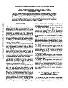
4 of 1-D chains as in constructing the 2-D AKLT resource, analyzing 2-D weighted graph state [7, 8], and weaving quantum wires into quantum webs [24]. In this scheme, one can always (a) isolate several usually horizontal, 1-D, universal chains from the 2-D state and (b) couple the correlation space of two neighboring 1-D chains whenever necessary. Resources of this type can be transformed to 2-D cluster state. To see this, one first isolate 1-D chain states from it; use the reductions we already have for the 1-D case to obtain 1-D cluster states; and then employ an appropriate coupling to link the 1-D cluster states into a two dimensional cluster state. The first two steps are obvious, while the third step is possible as shown in Fig. 3. In this figure, A[x]’s are defining matrices of cluster state chosen to be A[0] = |+ih0|, A[1] = |−ih1|, and B, C are tensors in the notion of Refs. [7, 8] B[0] = |+ir h0|l ⊗ |+id ,

B[1] = |−ir h1|l ⊗ |−id ,

C[0] = |+ir h0|l ⊗ |0iu ,

C[1] = |−ir h1|l ⊗ |1iu .

The Hadamard gates and the CZ gate |0ih0| ⊗ I + |1ih1| ⊗ Z, are implemented on the correlation spaces. The right hand side of Fig. 3 represents two nodes of degree 3 of a cluster state. A[x]

H

B[x]

H

∝ A[y]

H

H

C[y]

FIG. 3. Reduction of 2D resources of the coupling scheme

In the weighted graph state, for example, the isolated wire has the form HZ x S z where z depends on the outcomes of neighboring sites [7, 8]. We can measure all sites with odd z in the 0-1 basis and the resulting state is a 1-D cluster state up to random Clifford byproduct operations. The CZ gate can be applied in the same way as in Ref. [8]. Other coupling based schemes mentioned above can be analyzed in a similar way. Discussions.—The method of reduction for proving universality of MBQC resource state is applicable to other examples that have not been covered in the previous sections. These include, for example, the modified AKLT state (H, X, Y ) proposed in Ref. [7] and the second toric code state example in Ref. [8]. At the current stage, however, we do not know how one can reduce the first toric code example to the 2-D cluster state. It is worth comparing the idea of reduction and that of the “universal state preparator” result of Ref. [21]. A reduction to cluster state would imply the universal preparator property of the resource. On the other hand, although any universal preparator could in principle be transformed to a cluster state, the transformation does not respect the underlying lattice of the resource and may be less efficient than the quantum state reduction we are considering. For example, in the 1-D case, the method in Ref. [21] isolates a single particle of the physical space while reduction of 1-D resource results in again a

1-D state. And in the 2-D case, the preparator method will need polynomial cost to obtain a 2-D cluster state while state reduction remains of constant cost. The tabular form we propose is well hinged to the structure and properties of MPS. It simplifies the analysis by hiding the unwanted details and provides an intuitive way of manipulating the matrices. We have mainly investigated reductions of MPS and PEPS resources, but the idea seems to be able to generalize to potentially new MBQC scheme not known yet. It’s also reasonable to believe that investigations of the reduction method will improve our understanding of both the MBQC itself and the structure of universal resource states. RD is partly supported by QCIS, University of Technology, Sydney, and the NSF of China (Grant Nos. 60736011 and 60702080). ZJ acknowledges support from NSF of China (Grant Nos. 60736011 and 60721061). BZ is supported by NSERC and QuantumWorks. Research at Perimeter Institute is supported by the Government of Canada through Industry Canada and by the Province of Ontario through the Ministry of Research & Innovation.

[1] R. Raussendorf and H. J. Briegel, Phys. Rev. Lett. 86, 5188 (2001). [2] H. J. Briegel and R. Raussendorf, Phys. Rev. Lett. 86, 910 (2001). [3] Y.-Y. Shi, L.-M. Duan, and G. Vidal, Phys. Rev. A 74, 022320 (2006). [4] G. Vidal, Phys. Rev. Lett. 91, 147902 (2003). [5] D. Gross, S. T. Flammia, and J. Eisert, Phys. Rev. Lett. 102, 190501 (2009). [6] M. J. Bremner, C. Mora, and A. Winter, Phys. Rev. Lett. 102, 190502 (2009). [7] D. Gross and J. Eisert, Phys. Rev. Lett. 98, 220503 (2007). [8] D. Gross, J. Eisert, N. Schuch, and D. Perez-Garcia, Phys. Rev. A 76, 052315 (2007). [9] D. Perez-Garcia, F. Verstraete, M. M. Wolf, and J. I. Cirac, Quant. Inf. Comp. 7, 401 (2007). [10] M. Fannes, B. Nachtergaele, and R. F. Werner, Commun. Math. Phys. 144, 443 (1992). [11] F. Verstraete and J. I. Cirac, arXiv:cond-mat/0407066. [12] F. Verstraete, M. M. Wolf, D. Perez-Garcia, and J. I. Cirac, Phys. Rev. Lett. 96, 220601 (2006). [13] G. K. Brennen and A. Miyake, Phys. Rev. Lett. 101, 010502 (2008). [14] X. Chen, B. Zeng, Z.-C. Gu, B. Yoshida, and I. L. Chuang, Phys. Rev. Lett. 102, 220501 (2009). [15] M. A. Nielsen, Rep. Math. Phys. 57, 147 (2006). [16] M. V. den Nest, W. Dür, A. Miyake, and H. J. Briegel, New J. Phys. 9, 204 (2007). [17] H. J. Briegel, D. E. Browne, W. Dür, R. Raussendorf, and M. V. den Nest, Nat. Phys. 5, 19 (2009). [18] C. H. Bennett, H. J. Bernstein, S. Popescu, and B. Schumacher, Phys. Rev. A 53, 2046 (1996). [19] M. A. Nielsen, Phys. Rev. Lett. 83, 436 (1999). [20] W. Dür, G. Vidal, and J. I. Cirac, Phys. Rev. A 62, 062314 (2000). [21] J.-M. Cai, W. Dür, M. V. den Nest, A. Miyake, and H. J. Briegel, Phys. Rev. Lett. 103, 050503 (2009).

5 [22] I. Affleck, T. Kennedy, E. H. Lieb, and H. Tasaki, Phys. Rev. Lett. 59, 799 (1987). [23] I. Affleck, T. Kennedy, E. H. Lieb, and H. Tasaki, Commun. Math. Phys. 115, 477 (1988). [24] D. Gross and J. Eisert, arXiv:0810.2542. [25] D. Gross, Ph.D. thesis, Imperial College London (2008).

Appendix A: Reduction of triCluster state

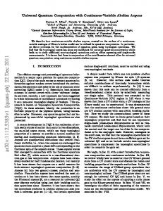
The triCluster state considered in Ref. [14] is a universal resource state of local dimension 6 and is the unique ground state of a two body, frustration-free, gapped Hamiltonian. We give a detailed reduction from the triCluster to cluster state in this appendix. The most concise way of describing the triCluster state is to employ the PEPS picture [12]. As in Fig. 4, each bond is the state |Hi ∝ |+i|0i + |−i|1i and each dashed circle is the projection P = P0 + P1 + P2 where |±i ∝ |0i ± |1i and P0 = |0ih000| + |1ih111|, P1 = |2ih001| + |3ih110|,

P2 = |4ih010| + |5ih101|.

X

Z

FIG. 4. Reduction of triCluster state to cluster state

One can transform the triCluster state into a cluster state on the same lattice, by simply measuring each site with Qj = Pj Pj† for j = 0, 1, 2. Although the outcomes will be random, one can assume that we have always measured 0, thereby only P0 are used for the projection on each site, except that there will be some random X errors happening on the bonds before the application of projections. As the action of X on one end of the bond |Hi is equivalent to a Z on the other end, we can propagate all X’s to neighboring sites as Z’s on the bond, which is the same as Z’s on the physical space. In conclusion, we have obtained the cluster state up to some Z errors determined by the random outcomes.

Appendix B: On the synchronization problem in the coupling method

We have discussed the reduction for a large class of 2-D resources made out of 1-D state by the coupling method. There is, however, a tricky point that we have overlooked. This appendix aims to convey the general idea that the problem is solvable. Imagine that we first isolate two neighboring chains, reduce them to 1-D cluster separately and then try to connect them into a 2-D cluster. Because of the randomness of the measurements, it may happen that the two chains are not both ready for the interaction if they are not aligned to the same column. That is, one chain contains more unmeasured particles than the other. To solve this synchronization problem, one may measure along these two chains in the basis that will induce the error-group random walk. Let us consider a simple example where the error group is hH, Zi and the interaction implemented is the CZ gate. The random walk is the Markov chain on the graph depicted in Fig. 5. The Markov chain is of period 2, meaning that it will only return to the starting state after even number of steps. Now the measurements on the two chains induce two independent random walk. If the difference of the number of unmeasured particles is even, the two random walks will be in the state I simultaneously after a finite number of steps. Otherwise, they will never be I simultaneously because of the periodicity of the Markov chain. However, one can wait a finite steps for the configuration of I and Z. The Z operation can commute with the CZ interaction and amounts to a byproduct for future steps of the reduction. I

H

HZ

X

Z

HX

HY

Y

FIG. 5. Random walk on the error group hH, Zi

A similar argument will work for the case where Z is a generator of the error group and the interaction implemented is CZ. As Z is a generator, the period of the random walk is either 1 or 2, and the synchronization problem can be dealt with similarly.