Query Rewriting and Optimization for Ontological Databases

Query Rewriting and Optimization for Ontological Databases

arXiv:1405.2848v1 [cs.DB] 12 May 2014

GEORG GOTTLOB, University of Oxford GIORGIO ORSI, University of Oxford ANDREAS PIERIS, University of Oxford

Ontological queries are evaluated against a knowledge base consisting of an extensional database and an ontology (i.e., a set of logical assertions and constraints which derive new intensional knowledge from the extensional database), rather than directly on the extensional database. The evaluation and optimization of such queries is an intriguing new problem for database research. In this paper, we discuss two important aspects of this problem: query rewriting and query optimization. Query rewriting consists of the compilation of an ontological query into an equivalent first-order query against the underlying extensional database. We present a novel query rewriting algorithm for rather general types of ontological constraints which is well-suited for practical implementations. In particular, we show how a conjunctive query against a knowledge base, expressed using linear and sticky existential rules, that is, members of the recently introduced Datalog± family of ontology languages, can be compiled into a union of conjunctive queries (UCQ) against the underlying database. Ontological query optimization, in this context, attempts to improve this rewriting process so to produce possibly small and cost-effective UCQ rewritings for an input query. Categories and Subject Descriptors: H.2.4 [Database Management]: Systems — query processing, rulebased databases, relational databases; I.2.3 [Artificial Intelligence]: Deduction and Theorem Proving — inference engines, logic programming, resolution General Terms: Algorithms, Theory, Languages, Performance Additional Key Words and Phrases: Ontological query answering, tuple-generating dependencies, query rewriting, query optimization

1. INTRODUCTION 1.1. Ontological Database Management Systems

The use of ontological reasoning in companies, governmental organizations, and other enterprises has become widespread in recent years. An ontology is an explicit specification of a conceptualization of an area of interest, and consists of a formal representation of knowledge as a set of concepts within a domain, and the relationships between instances of those concepts. Moreover, ontologies have been adopted as high-level conceptual descriptions of the data contained in data repositories that are sometimes distributed and heterogeneous in the data models. Due to their high expressive power, ontologies are also replacing more traditional conceptual models such as UML class diagrams and Entity Relationship schemata. We are currently witnessing the marriage of ontological reasoning and database technology, which gives rise to a new type of database management systems, the socalled ontological database management systems, equipped with advanced reasoning and query processing mechanisms [Calvanese et al. 2007; Cal`ı et al. 2011]. More precisely, an extensional database D is combined with an ontology Σ which derives new intensional knowledge from the extensional database. An input conjunctive query is not just answered against the database, as in the classical setting, but against the logical theory (a.k.a. ontological database) D ∪ Σ — recall that conjunctive queries correspond to the select-project-join fragment of relational algebra, and form one of the most natural and commonly used languages for querying relational databases [Abiteboul et al. 1995]. Therefore, the answer to a conjunctive query ∃Y ϕ(X, Y) with distinguished variables X over the ontological database consists of all tuples t of constants such that, when we substitute the variables X with t, ∃Yϕ(t, Y) evaluates to true in every model of D ∪ Σ, i.e., in every instance which contains D and satisfies Σ.

2

This amalgamation of different technologies stems from the need for semantically enhancing existing databases with ontological constraints. Indeed, database technology providers have recognized this need, and have recently started to build ontological reasoning modules on top of their existing software with the aim of delivering effective database management solutions to their customers. For example, Oracle Inc. offers a system, called Oracle Database 11g, enhanced by modules performing ontological reasoning tasks1 . Also, Ontotext offers a family of semantic repositories, called OWLIM2 , and Semafora Systems develops an inference machine, called Ontobroker3 , for processing ontologies that support all of the World Wide Web Consortium (W3C) recommendations. Enhancing databases with ontologies is also at the heart of several research-based systems such as QuOnto [Acciarri et al. 2005] and Quest [Rodriguez-Muro and Calvanese 2012]. 1.2. Ontology Languages

Ontologies are modeled using formal languages called ontology languages. Description Logics (DLs) [Baader et al. 2003] are a family of knowledge representation languages widely used in ontological modeling. In fact, DLs model a domain of interest in terms of concepts and roles, which represent classes of individuals and binary relations on classes of individuals, respectively. Interestingly, DLs provide the logical underpinning for the Web Ontology Language (OWL), and its revision OWL 2, as standartized by the W3C4 . Unfortunately, in order to achieve favorable computational properties, DLs are able only to describe knowledge for which the underlying relational structure is treelike. Moreover, they usually support only unary and binary relations. The overcoming of the above limitations, through the definition of expressive rule-based ontology languages, has become the last years a field of intense research in the KR and database communities. In fact, traditional database constraints such as tuple-generating dependencies (TGDs) (a.k.a. existential rules and Datalog± rules) of the form ∀X∀Y ϕ(X, Y) → ∃Z ψ(X, Z), where ϕ and ψ are conjunctions of atoms over a relational schema, appeared to be a suitable formalism for ontological modeling and reasoning — examples of such languages can be found in [Baget et al. 2011; Krötzsch and Rudolph 2011; Cal`ı et al. 2012a; Cal`ı et al. 2012b]. A vital computational property of an ontology language, apart from ensuring the decidability, is to guarantee the tractability of conjunctive query answering w.r.t. the data complexity, i.e., the complexity calculated by considering only the database as part of the input. Indeed, the data complexity of query answering is widely regarded as more meaningful and relevant in practice than the combined complexity (calculated by considering everything as part of the input), since the query and the ontology are typically of a size that can be productively assumed to be fixed, and usually are much smaller than a typical relational database. Several lightweight DLs have been proposed which guarantee that conjunctive query answering is feasible in polynomial time w.r.t. the data complexity. Such DLs are EL [Baader 2003] and the members of the DL-Lite family [Calvanese et al. 2007; Poggi et al. 2008], i.e., DL-LiteR , DL-LiteF and DL-LiteA . These languages can be seen as tractable sublanguages of OWL; in fact, the language DL-LiteR forms the OWL 2 QL5 profile of OWL 2. It was convincingly argued that, despite their simplicity, EL and the DL-Lite formalisms are powerful enough for modeling an overwhelming number of real-life scenarios. More re1 http://www.oracle.com/technetwork/database/enterprise-edition/overview/index.html 2 http://www.ontotext.com/owlim 3 http://www.semafora-systems.com/en/products/ontobroker/ 4 http://www.w3.org/TR/owl2-overview/ 5 http://www.w3.org/TR/owl2-profiles/

Query Rewriting and Optimization for Ontological Databases conjunctive query

ontology

q

Σ

3

compilation

qΣ positive first-order query

translation

q⋆

evaluation

non-recursive SQL query

D

extensional database

Fig. 1. Answering queries via rewriting.

cently, several classes of TGDs have been identified which guarantee the same low data complexity for conjunctive query answering. For example, the class of guarded TGDs, inspired by the guarded fragment of first-order logic [Andréka et al. 1998], which is noticeably more general than EL and the members of the DL-Lite family, has been investigated in [Cal`ı et al. 2008] — extensions of guarded TGDs can be found in [Baget et al. 2011; Krötzsch and Rudolph 2011]. Moreover, the classes of linear and sticky TGDs, which both encompass the DL-Lite family, have been proposed in [Cal`ı et al. 2012a] and [Cal`ı et al. 2012b]. 1.3. First-Order Rewritability

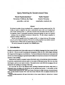
Polynomial time tractability is often considered not to be good enough for efficient query processing. Ideally, one would like to achieve the same complexity as for processing first-order queries, or, equivalently, (non-recursive) SQL queries. An ontology language L guarantees the first-order rewritability of conjunctive query answering if, for every conjunctive query q and ontology Σ expressed in L, a positive first-order query qΣ , called perfect rewriting6, can be constructed such that, given a database D, qΣ evaluated over D yields exactly the same result as q evaluated against the ontological database D ∪ Σ [Calvanese et al. 2007]. Since answering first-order queries is in AC0 in data complexity [Vardi 1995], it immediately follows that query answering under ontology languages that guarantee the first-order rewritability of the problem is also in AC0 in data complexity. First-order rewritability is a most desirable property since it ensures that the query answering process can be largely decoupled from data access. In fact, as depicted in Figure 1, to answer a query q over an ontological database D ∪ Σ, a separate software can compile q into qΣ , then translate qΣ into a standard SQL query q ⋆ , and finally submit it to the underlying relational database management system holding D, where it is evaluated and optimized in the usual way. Example 1.1. Consider the set Σ consisting of the TGD: ∀X∀Y project (X), inArea(X, Y ) → ∃Z hasCollaborator (Z, Y, X), asserting that each project has an external collaborator specialized in the area of the project. We can ask for projects in the area of databases for which there are external collaborators by posing the CQ ∃A hasCollaborator (A, db, B). Intuitively, due to the 6 In

general, there exist more than one perfect rewritings. However, for query answering, all the possible rewritings are equivalent, and thus we can refer to the perfect rewriting.

4

SELECT C.p id FROM hasCollaborator C WHERE C.area = ’db’ UNION SELECT P.p id FROM project P, inArea A WHERE A.area = ’db’ AND P.p id = A.p id. Fig. 2. The SQL query of Example 1.1.

above TGD, not only we have to query hasCollaborator , but we also need to look for projects in the area of databases, as such projects will necessarily have an external collaborator. The perfect rewriting qΣ will thus be the union of CQs: (∃A hasCollaborator (A, db, B)) ∨ (project (B) ∧ inArea(B, db)) . Assuming the schema project (p id), inArea(p id, area), hasCollaborator (c id, area, p id), it is clear that qΣ can be written in SQL as shown in Figure 2. Interestingly, the members of the DL-Lite family of DLs, as well as the classes of linear and sticky TGDs, guarantee the first-order rewritability of conjunctive query answering. Actually, the above languages guarantee a stronger property than first-order rewritability: given a conjunctive query q, and an ontology Σ expressed in one of the above formalisms, the perfect rewriting qΣ can be expressed as a union of conjunctive queries, i.e., we do not need the full expressive power of positive first-order queries. As we explain below, the main problem that we address in this paper is precisely the question of how to compute qΣ correctly and efficiently, when the input ontology Σ is expressed as a set of linear or sticky TGDs. 1.4. Aims and Objectives

The advantage of first-order rewritability is obvious, that is, conjunctive query answering can be deferred to a standard query language such as SQL, which in turn allows us to exploit mature and efficient existing database technology that is accessible via the underlying database management system. However, there is a drawback in this approach: if the algorithm which constructs the perfect rewriting inflates the query excessively, and creates from a reasonably sized ontological query a massive exponentially sized SQL query, then even the best database management system may be of little use. This problem gave rise to a flourishing research activity in the DL community. A remarkable number of rewriting algorithms, with the aim of compiling a conjunctive query and a DL-Lite ontology into a “small” union of conjunctive queries, have been proposed the last five years (see, e.g., [Calvanese et al. 2007; Pérez-Urbina et al. 2010; Chortaras et al. 2011; Kikot et al. 2012a; Venetis et al. 2013]) — see Section 2. Surprisingly, before the conference version of the present paper [Anonymous ], no practical algorithm, able to efficiently compile a conjunctive query and an ontology modeled using an expressive TGD-based language into a union of conjunctive queries, was available. It is the precise aim of this work to fill this gap for linear and sticky TGDs. Both linearity and stickiness are well-accepted paradigms: — A TGD is called linear if it has only one body-atom [Cal`ı et al. 2012a]; notice that the body is the left-hand side of the implication. Despite its simplicity, linearity forms a robust language with several applications. Linear TGDs are strictly more expressive than the description logic DL-LiteR [Calvanese et al. 2007] which, as already said, forms the OWL 2 QL profile of W3Cs standard ontology language for modeling Semantic Web ontologies. Importantly, linear TGDs, in contrast to DL-LiteR , can be used with relational database schemas of arbitrary ar-


5

ity. The usefulness of schemas of higher arity (not just unary and binary relations) has been recognized by the DL community, and as evident we mention DLRLite [Calvanese et al. 2013a], a recent generalization of DL-Lite to arbitrary arity, which is also captured by linear TGDs. Also, linear TGDs generalize inclusion dependencies, a well-known class of relational constraints; in fact, inclusion dependencies can be equivalently written as TGDs with just one body-atom and one head-atom without repeated variables. Moreover, linear TGDs are powerful enough to express conditional inclusion dependencies which extend traditional inclusion dependencies by enforcing bindings of semantically related data values, and they are useful in data cleaning and contextual schema mapping [Bohannon et al. 2006; Bravo et al. 2007]; in fact, conditional inclusion dependencies can be written as linear TGDs with constant values in the body. Furthermore, linear TGDs generalize local-as-view (LAV) TGDs which are employed in data exchange and data integration to define schema mappings, i.e., specifications that describe how data for a source schema can be transformed into data for a target schema; see, e.g., [ten Cate and Kolaitis 2009]. Finally, linear TGDs can be used in schema evolution, and in particular for expressing the decompose operator, with the aim of splitting a table into smaller tables [Curino et al. 2013]. — Stickiness [Cal`ı et al. 2012b] allows joins to appear in rule-bodies which are not expressible via linear TGDs, let alone via DL(R)-Lite assertions; more details are given in Section 3. Interestingly, sticky TGDs are able to capture well-known data modeling constructs such as (conditional) inclusion and multivalued dependencies. Furthermore, sticky TGDs, in contrast to linear TGDs (and most of the existing DLs) allow to describe knowledge for which the underlying relational structure is not treelike. This is mainly due to the fact that sticky TGDs are expressive enough for encoding the cartesian product of two tables; e.g., the set of sticky TGDs consisting of ∀X∀Y pi (X, Y ) → ∃Z pi (Y, Z), si (Z), for each i ∈ {1, 2}, and ∀X∀Y s1 (X), s2 (Y ) → r(X, Y ), computes the cartesian product of s1 and s2 which forms an infinite clique, and thus the underlying relational structure has infinite treewidth. As already observed by the DL community, there are some natural ontological statements, e.g., “all elephants are bigger than all mice” [Rudolph et al. 2008], which are expressible only via cartesian product assertions. Notice that the above statement can be captured by the sticky TGD ∀X∀Y elephant (X), mouse(Y ) → biggerThan (X, Y ). Finally, sticky TGDs can also be used for schema evolution purposes, and in particular for expressing the merge operator, with the aim of putting together two or more tables [Curino et al. 2013]. Apart from designing a practical rewriting algorithm for linear and sticky TGDs, we would also like to investigate the possibility of improving the computation of the perfect rewriting on multi-core architectures commonly available in modern database servers. On the long term, we envision relational database systems able to handle ontological constraints natively, as it is done today for traditional data dependencies such as primary and foreign keys. A key difference is that ontological constraints are not supposed to be enforced by the DBMS as classical integrity constraints, but rather to be taken into consideration during the evaluation of a query. This paper is a significant step towards this direction. 1.5. The Existing Approach

Although it is known that both linear and sticky TGDs guarantee the first-order rewritability of conjunctive query answering, the existing algorithms are of theoretical nature, and it is generally accepted that there is no obvious way how they will lead to better practical rewriting algorithms. The key property of linear and sticky

6

TGDs which implies the first-order rewritability of conjunctive query answering is the so-called bounded derivation-depth property (BDDP) [Cal`ı et al. 2012a]. As we shall see in Section 3, to compute the answer to a conjunctive query q over an ontological database D ∪ Σ, where Σ is a linear or sticky ontology, it suffices to evaluate q over a special model of D ∪ Σ which can be homomorphically embedded into every other model of D ∪ Σ. Such a model, called universal model (a.k.a. canonical model), always exists and can be constructed by applying the chase procedure, a powerful tool for reasoning about data dependencies — intuitively, the chase adds new atoms to the extensional database D, possibly involving null values which act as witnesses for the existentially quantified variables, until the final result, denoted chase(D, Σ), satisfies Σ. However, chase(D, Σ) is in general infinite, and thus not explicitly computable. The BDDP implies that it suffices to evaluate q over an initial finite part of chase(D, Σ) which depends only on q and Σ. Roughly, chase(D, Σ) can be decomposed into levels, where database atoms have level zero, while an inferred atom has level k + 1 if it is obtained due to atoms with maximum level k; we refer to the part of the chase up to level k as chase k (D, Σ). Thus, the BDDP implies that there exists k > 0 such that, for every database D, the answer to q over D∪Σ coincides with the answer to q over chase k (D, Σ). An algorithm for computing the prefect rewriting qΣ by exploiting the above property has been presented in [Cal`ı et al. 2012a]. Roughly, one can enumerate all the possible database ancestors D1 , . . . , Dn of the image of the given query, and then, starting from each Di , construct chase k (D, Σ), where k is the depth provided by the BDDP, which will give rise to a query in the final rewriting. It is evident that such a procedure is computationally expensive, and also the obtained queries are usually very large and cannot be effectively materialized. Notice that the goal of [Cal`ı et al. 2012a] was to establish that classes of TGDs which enjoy the BDDP guarantee the first-order rewritability of conjunctive query answering, without taking into account implementation issues. It is apparent that we had to look for new rewriting procedures which substantially deviate from the one described above. 1.6. Summary of Contributions

Our contributions can be summarized as follows: (1) We propose a novel query rewriting algorithm, called XRewrite, which is based on backward-chaining resolution. In fact, XRewrite uses the TGDs as rewriting rules, with the aim of simulating, independently from the extensional database, the chase derivations which are responsible for the generation of the image of the input query. Such an algorithm is better for practical applications than the one described above since, during the rewriting process, we only explore the part of the chase which is needed in order to entail the query, i.e., the proof of the query, and thus we avoid the generation of a non-negligible number of useless atoms. Interestingly, XRewrite is sound and complete even if we consider an arbitrary set of TGDs without any syntactic restrictions; however, in this general case, the termination of the algorithm is not guaranteed. We show that, if the input set of TGDs is linear or sticky, then XRewrite terminates, and thus it forms a practical query rewriting algorithm for linear and sticky TGDs; recall that the designing of such an algorithm is the main research challenge of this work. (2) We present a parallel version of XRewrite, called XRewriteParallel, with the aim of reducing the overall execution time for computing the final rewriting by exploiting multi-core architectures. To the best of our knowledge, this is the first attempt to design a parallel query rewriting algorithm. The key idea is to decompose the input query q into smaller queries q1 , . . . , qm , where m > 1, in such a way that each qi


7

can be rewritten independently by concurrent rewriters into a query Qqi , and then merge the queries Qq1 , . . . , Qqm in order to obtain the final rewriting. (3) We propose a technique, called query elimination, aiming at optimizing the final rewritten query under linear TGDs. Query elimination, which is an additional step during the execution of XRewrite, reduces (i) the size of the final rewriting, (ii) the number of atoms in each query of the rewriting, and (iii) the number of joins to be executed. The key idea underlying query elimination is that the linearity of TGDs allows us to effectively identify atoms in the body a query which are logically implied (w.r.t. a given set of TGDs) by other atoms in the same query. (4) After implementing our algorithm, we have analyzed its behavior, and we have spotted certain operations, such as the computation of the most general unifier for a set of atoms, that might benefit from caching. We also perform an extensive analysis on the impact of our optimizations on the rewriting process, and we show that all of them reduce the number of redundant queries in the final rewriting. We finally compare our system with A LASKA (i.e., the reference implementation of [König et al. 2012]) which is the only known system which supports ontological query rewriting under arbitrary TGDs. We observe that both systems return minimal rewritings on the given test cases. However, query elimination allows us to perform a better exploration of the rewriting search space on most of the given test cases. Interestingly, even for the cases where A LASKA performs a better exploration of the search space, our algorithm achieves better performance due to the caching mechanism. Notably, on certain test cases, the parallelization of the rewriting provides a fundamental contribution towards making the rewriting manageable as the number of explored and generated queries is drastically reduced. Roadmap. After a review of previous work on query rewriting in Section 2, and some technical definitions and preliminaries in Section 3, we proceed with our new results. In Section 4, we present the rewriting algorithm XRewrite, and in Section 5 its parallel version. In Section 6, we present the query elimination technique. Implementation issues are discussed in Section 7, while the experimental evaluation is presented in Section 8. We conclude in Section 9 with a brief outlook on further research. 2. RELATED WORK ON QUERY REWRITING

An early query rewriting algorithm for the DL-Lite family of DLs, introduced in [Calvanese et al. 2007] and implemented in the QuOnto system, reformulates the given query into a union of conjunctive queries. The size of the reformulated query is unnecessarily large. This is mainly due to the fact that the factorization step (which is needed, as we shall see, to guarantee completeness) is applied in a “blind” way, even if it is not needed, and as a result many superfluous queries are generated. In [Pérez-Urbina et al. 2010] an alternative resolution-based rewriting algorithm for DL-LiteR is proposed, implemented in the Requiem system, that addressed the issue of the useless factorizations (and therefore of the redundant queries generated due to this weakness) by directly handling existential quantification through proper functional terms — notice that this algorithm works also for more expressive DLs, which do not guarantee first-order rewritability of query answering; in this case, the computed rewriting is a (recursive) Datalog query. A query rewriting algorithm for DLLiteR , called Rapid, which is more efficient than the one in [Pérez-Urbina et al. 2010], is presented in [Chortaras et al. 2011]. The efficiency of Rapid is based on the selective and stratified application of resolution rules; roughly, it takes advantage of the query structure and applies a restricted sequence of resolutions that may lead to useful and redundant-free rewritings. An alternative query rewriting technique for DL-LiteR is

8

presented in [Kikot et al. 2012a] — although the obtained rewritings are, in general, not correct and of exponential size, in most practical cases the rewritings are correct and of polynomial size. In [Venetis et al. 2013], the problem of computing query rewritings for DL-LiteR in an incremental way is investigated. More precisely, a technique which computes an extended query by “extending” a previously computed rewriting of the initial query (and thus avoiding recomputation) is proposed. The algorithms mentioned above leverage specificities of DLs, such as the limit to unary and binary predicates only and the absence of variable permutations in the axioms. Therefore, they cannot be easily extended to more general TGD-based languages; in fact, DL-based systems often resort to case-by-case analysis on the syntactic form of the DL axioms. Following a more general approach, the works [Anonymous ; König et al. 2012; König et al. 2013] presented a backward-chaining rewriting algorithm which is able to deal with arbitrary TGDs, providing that the language under consideration satisfies suitable syntactic restrictions that guarantee the termination of the algorithm. Other works, which follow a different approach, and instead of computing a union of conjunctive queries the rewritings are expressed in some other query language, such as non-recursive Datalog, can be found in the literature [Rosati and Almatelli 2010; Orsi and Pieris 2011; Gottlob and Schwentick 2012; Kikot et al. 2012b; Thomazo 2013]. A distantly related research field is that of database query reformulation in presence of views and constraints [Deutsch et al. 1999; Halevy 2001]. Given a conjunctive query q, and a set of constraints Σ, the goal is to find all the minimal equivalent reformulations of q w.r.t. Σ. The most interesting approach in this respect is the chase & backchase algorithm [Deutsch et al. 1999], implemented in the MARS system [Deutsch and Tannen 2003]. The relationship of the chase & backchase algorithm with this work is discussed in Section 6. 3. DEFINITIONS AND BACKGROUND 3.1. Technical Definitions

We present background material necessary for this paper. We recall some basics on relational databases, relational queries, tuple-generating dependencies, and the chase procedure relative to such dependencies. For further details on the above notions we refer the reader to [Abiteboul et al. 1995]. Alphabets. We define the following pairwise disjoint (countably infinite) sets of symbols: a set Γ of constants (constitute the “normal” domain of a database), a set ΓN of labeled nulls (used as placeholders for unknown values, and thus can be also seen as (globally) existentially quantified variables), and a set ΓV of (regular) variables (used in queries and dependencies). Different constants represent different values (unique name assumption), while different nulls may represent the same value. A fixed lexicographic order is assumed on Γ ∪ ΓN such that every value in ΓN follows all those in Γ. We denote by X sequences (or sets, with a slight abuse of notation) of variables X1 , . . . , Xk , with k > 1. Throughout, let [n] = {1, . . . , n}, for any integer n > 1. Relational Model. A relational schema R (or simply schema) is a set of relational symbols (or predicates), each with its associated arity. We write r/n to denote that the predicate r has arity n. By arity(R) we refer to the maximum arity over all predicates of R. A position r[i] (in R) is identified by a predicate r ∈ R and its i-th argument (or attribute). A term t is a constant, null, or variable. An atomic formula (or simply atom) has the form r(t1 , . . . , tn ), where r/n is a relation, and t1 , . . . , tn are terms. For an atom a, we denote as terms(a) and var (a) the set of its terms and the set of its variables, respectively. These notations naturally extend to sets of atoms. Conjunctions of atoms are often identified with the sets of their atoms. An instance I for a schema R is a


9

(possibly infinite) set of atoms of the form r(t), where r/n ∈ R and t ∈ (Γ ∪ ΓN )n . A database D is a finite instance such that terms(D) ⊂ Γ. Substitutions. A substitution from a set of symbols S to a set of symbols S ′ is a function h : S → S ′ defined as follows: ∅ is a substitution (empty substitution), and if h is a substitution, then h ∪ {t → t′ } is a substitution, where t ∈ S and t′ ∈ S ′ ; if t → t′ ∈ h, then we write h(t) = t′ . An assertion of the form t → t′ is called mapping. The restriction of h to T ⊆ S, denoted h|T , is the substitution h′ = {t → h(t) | t ∈ T }. A homomorphism from a set of atoms A to a set of atoms A′ is a substitution h : Γ ∪ ΓN ∪ ΓV → Γ ∪ ΓN ∪ ΓV such that: if t ∈ Γ, then h(t) = t, and if r(t1 , . . . , tn ) ∈ A, then h(r(t1 , . . . , tn )) = r(h(t1 ), . . . , h(tn )) ∈ A′ . A set of atoms A = {a1 , . . . , an }, where n > 2, unifies if there exists a substitution γ, called unifier for A, such that γ(a1 ) = . . . = γ(an ). A most general unifier (MGU) for A is a unifier for A, denoted as γA , such that for each other unifier γ for A, there exists a substitution γ ′ such that γ = γ ′ ◦ γA . Notice that if a set of atoms unify, then there exists a MGU. Furthermore, the MGU for a set of atoms is unique (modulo variable renaming). Datalog. A Datalog rule ρ is an expression of the form a0 ← a1 , . . . , an , for n > 0, where ai is an atom containing constants of Γ and variables of ΓV , and every variable occurring in a0 must appear in at least one of the atoms a1 , . . . , an ; the latter is known as the safety condition. The atom a0 is called the head of ρ, denoted as head (ρ), while the set of atoms {a1 , . . . , an } is called the body of ρ, denoted as body(ρ). A Datalog program Π over a schema R is a set of Datalog rules such that, for each ρ ∈ Π, the predicate of head (ρ) does not occur in R. The program Π is non-recursive if there is some ordering ρ1 , . . . , ρn of the rules of Π so that the predicate in the head of ρi does not occur in the body of a rule ρj , for each j 6 i. The extensional database (EDB) predicates are those that do not occur in the head of any rule of Π; all the other predicates are called intensional database (IDB) predicates. A model of Π is an instance I for R such that, for every Datalog rule of the form a0 ← a1 , . . . , an appearing in Π, I satisfies the first-order formula ∀X(a1 ∧. . .∧an → a0 ), where X are the variables occurring in ρ. In other words, whenever there exists a homomorphism h such that h({a1 , . . . , an }) ⊆ I, h(a0 ) ∈ I. The semantics of Π w.r.t. a database D for R, denoted as Π(D), is the minimum model of Π containing D (which is unique and always exists). Queries. An n-ary Datalog query Q over a schema R is a pair hΠ, pi, where Π is a Datalog program over R, and p is an n-ary (output) predicate which occurs in the head of at least one rule of Π. Q is a non-recursive Datalog query if Π is non-recursive. Q is a union of conjunctive queries (UCQs) if Π is non-recursive, p is the only IDB predicate in Π, and for each rule ρ ∈ Π, p does not occur in body (ρ). Finally, Q is a conjunctive query (CQ) if it is a union of CQs, and Π contains exactly one rule. The answer to an n-ary Datalog query Q = hΠ, pi over a database D is the set {t ∈ Γn | p(t) ∈ Π(D)}, denoted Q(D). Since the output predicate of a (U)CQ is clear from the syntax of the query, in the rest of the paper, for brevity, a CQ is seen as a Datalog rule, while a UCQ is seen as a Datalog program (instead of a pair consisting of a program and a predicate). The variables occurring in the head of a CQ are its distinguished variables. The answer to a CQ q 7 over a (possibly infinite) instance I can be equivalently defined as the set of all tuples of constants t for which there exists a homomorphism h such that h(body(q)) ⊆ I and h(X) = t, where X are the distinguished variables of q. The answer to a UCQ Q over I can be equivalently defined as the set of tuples {t | there exists q ∈ Q such that t ∈ q(I)}. Tuple-Generating Dependencies. A tuple-generating dependency (TGD) σ over a schema R is a first-order formula ∀X∀Y ϕ(X, Y) → ∃Z ψ(X, Z), where X∪Y ∪Z ⊂ ΓV , and ϕ, ψ are conjunctions of atoms over R (possibly with constants). Formula ϕ is the 7 Henceforth,

for clarity, we usually use lower case letters for CQs and upper case letters for UCQs.

10

body of σ, denoted body (σ), while ψ is the head of σ, denoted head (σ). Henceforth, for brevity, we will omit the universal quantifiers in front of TGDs. Such σ is satisfied by an instance I for R, written I |= σ, if the following holds: whenever there exists a homomorphism h such that h(ϕ(X, Y)) ⊆ I, then there exists a homomorphism h′ ⊇ h|X , called extension of h|X , such that h′ (ψ(X, Z)) ⊆ I. An instance I satisfies a set Σ of TGDs, denoted I |= Σ, if I |= σ for each σ ∈ Σ. A set Σ of TGDs is in normal form if each of its TGDs has a single head-atom which contains only one occurrence of an existentially quantified variable. As shown, e.g., in [Cal`ı et al. 2012b], every set Σ of TGDs over a schema R can be transformed in logarithmic space into a set N(Σ) over a schema RN(Σ) in normal form of size at most quadratic in |Σ|, such that Σ and N(Σ) are equivalent w.r.t. query answering — for more details see Section A.1. Conjunctive Query Answering under TGDs. Given a database D for a schema R, and a set Σ of TGDs over R, the answers we consider are those that are true in all models of D w.r.t. Σ. Formally, the models of D w.r.t. Σ, denoted as mods(D, Σ), is the set of all instances I such that I ⊇ D and I |= Σ. The answer to an n-ary CQ q w.r.t. D and Σ, denoted as ans(q, D, Σ), is the set of n-tuples {t | t ∈ q(I), for each I ∈ mods(D, Σ)}; the answer to an n-ary UCQ is defined analogously. Notice that the associated decision problem, which asks whether a tuple of constants belongs to the answer of a CQ w.r.t. a database and a set of TGDs, is undecidable under arbitrary TGDs [Beeri and Vardi 1981]; in fact, it remains undecidable even when the schema and the set of TGDs are fixed [Cal`ı et al. 2008], or even when the set of TGDs is a singleton [Baget et al. 2011]. Concrete classes of TGDs which are of special interest for the current work, and also guarantee the decidability of query answering, are presented in Section 3.3. The TGD Chase Procedure. The chase procedure (or simply chase) is a fundamental algorithmic tool introduced for checking implication of dependencies [Maier et al. 1979], and later for checking query containment [Johnson and Klug 1984]. Informally, the chase is a process of repairing a database w.r.t. a set of dependencies so that the resulted instance satisfies the dependencies. By abuse of terminology, we shall use the term “chase” interchangeably for both the procedure and its result. The chase works on an instance through the so-called TGD chase rule: TGD chase rule. Consider an instance I for a schema R, and a TGD σ : ϕ(X, Y) → ∃Z ψ(X, Z) over R. We say that σ is applicable to I if there exists a homomorphism h such that h(ϕ(X, Y)) ⊆ I. The result of applying σ to I with h is I ′ = I ∪ h′ (ψ(X, Z)), and we write Ihσ, hiI ′ , where h′ is an extension of h|X such that h′ (Z) is a “fresh” labeled null of ΓN not occurring in I, and following lexicographically all those in I, for each Z ∈ Z. In fact, Ihσ, hiI ′ defines a single TGD chase step. Let us now give the formal definition of the chase of a database w.r.t. a set of TGDs. A chase sequence of a database D w.r.t. a set Σ of TGDs is a sequence of chase steps Ii hσi , hi iIi+1 , where i > 0, I0 = D and σi ∈ Σ. The chase of D w.r.t. Σ, denoted chase(D, Σ), is defined as follows: – A finite chase of D w.r.t. Σ is a finite chase sequence Ii hσi , hi iIi+1 , where 0 6 i < m, and there is no σ ∈ Σ which is applicable to Im ; let chase(D, Σ) = Im . – An infinite chase sequence Ii hσi , hi iIi+1 , where i > 0, is fair if whenever a TGD σ : ϕ(X, Y) → ∃Z ψ(X, Z) is applicable to Ii with homomorphism h, then there exists an extension h′ of h|X and k > i such that h′ (head (σ)) ⊆ Ik . An infinite chase of DSw.r.t. Σ ∞ is a fair infinite chase sequence Ii hσi , hi iIi+1 , where i > 0; let chase(D, Σ) = i=0 Ii . Let chase [k] (D, Σ) be the instance constructed after k > 0 applications of the TGD chase step. An example of the chase procedure can be found in Section A.1. It is


11

well-known that the chase of D w.r.t. Σ is a universal model of D w.r.t. Σ, i.e., for each I ∈ mods(D, Σ), there exists a homomorphism hI such that hI (chase(D, Σ)) ⊆ I [Fagin et al. 2005; Deutsch et al. 2008]. Using this universality property, it can be shown that the chase is a formal algorithmic tool for query answering under TGDs. More precisely, the answer to a CQ q w.r.t. a database D and a set of TGDs Σ coincides with the answer to q over the chase of D w.r.t. Σ, i.e., ans(q, D, Σ) = q(chase(D, Σ)). The TGD chase rule given above is known as oblivious since it “forgets” to check whether the TGD under consideration is already satisfied, i.e., it adds atoms to the given instance even if it is not necessary. The version of the TGD chase rule which applies stricter criteria to the applicability of TGDs, with the aim of adding atoms to the given instance only if it is necessary, is called restricted. The universality property was originally shown for the restricted version of the chase [Fagin et al. 2005; Deutsch et al. 2008], which is considered as the standard one. However, as explicitly stated in [Cal`ı et al. 2013], the universality property holds also for the oblivious chase; this was established by showing the existence of a homomorphism from the oblivious to the restricted chase. Thus, for our purposes, we can safely consider the oblivious chase. This is done for technical clarity and simplicity. As discussed in [Johnson and Klug 1984], even in the simple case of inclusion dependencies, things become technically more complicated if the restricted chase is employed, since the applicability of a TGD depends on the presence of other atoms previously constructed by the chase. 3.2. Query Answering via Rewriting

A fundamental property that a class of TGDs should enjoy is to guarantee the decidability of (the decision version) of conjunctive query answering; recall that in general this problem is undecidable. However, as already discussed in Section 1, to be able to work with very large data sets, decidability of query answering is not enough. We need also high tractability in data complexity, i.e., when both the query and the set of TGDs are fixed, and possibly feasible by the use of relational query processors. First-order rewritability, introduced in the context of description logics [Calvanese et al. 2007], guarantees the above desirable properties. Roughly speaking, given a CQ and a set of TGDs, a (finite) first-order query can be constructed, called perfect rewriting, that takes into account the semantic consequences of the TGDs. Then, the answer to the input query w.r.t. a database D and the set of TGDs is obtained by evaluating the perfect rewriting directly over D. Formally, the problem of conjunctive query answering under a set of TGDs Σ is first-order rewritable if, for every CQ q, a (finite) positive first-order query qΣ can be constructed such that, for every database D, ans(q, D, Σ) = qΣ (D). Unfortunately, the problem of deciding whether a set of TGDs guarantees the first-order rewritability of CQ answering is undecidable; for more details see Section A.2. It is well-known that the evaluation of first-order queries is in the highly tractable class AC 0 in data complexity [Vardi 1995]. Recall that this is the complexity class of recognizing words in languages defined by constant-depth Boolean circuits with (unlimited fan-in) AND and OR gates (see, e.g., [Papadimitriou 1994]). Consequently, CQ answering under sets of TGDs which guarantee the first-order rewritability of the problem is in AC0 in data complexity. Given that every first-order query can be equivalently written in (non-recursive) SQL, in practical terms this means that CQ answering can be deferred to a standard query language such as SQL. This allows us to exploit all the optimization capabilities of the underlying RDBMS. 3.3. Concrete Classes of TGDs

Since the problem of identifying first-order rewritability is undecidable, it is not possible to syntactically characterize the fragment of TGDs which guarantees the first-

12

r(X,Y),p(Y,Z) → ∃W t(X,Y,W)

σ1 : r(X,Y) → ∃Z r(Y,Z)

t(X,Y,Z) → ∃W s(Y,W)

σ4 : r(X,Y),r(Z,X) → s(X)

√

r(X,Y),p(Y,Z) → ∃W t(X,Y,W) σ1 : r(X,Y) → ∃Z r(Y,Z) t(X,Y,Z) → ∃W s(X,W) × (a)

(b)

Fig. 3. Sticky property and propagation step.

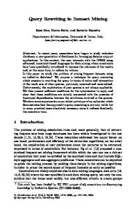
order rewritability of CQ answering. However, several sufficient syntactic conditions have been proposed — the two main conditions are linearity and stickiness. Linearity. Linear TGDs have been proposed in [Cal`ı et al. 2012a]. A TGD σ is called linear if σ has only one body-atom. The class of linear TGDs, i.e., the set of all possible sets of linear TGDs, is denoted LINEAR. Despite its simplicity, as already discussed in Section 1.4, LINEAR is quite natural with several applications. Linear TGDs guarantee the first-order rewritability of CQ answering [Cal`ı et al. 2012a]; this is also implicit in [Baget et al. 2011], where atomic-hypothesis rules, which coincide with linear TGDs, are investigated. This result was established by showing that LINEAR enjoys the BDDP. However, as already remarked in Section 1, the techniques based on the BDDP do not lead to practical query rewriting algorithms. Stickiness. The class of sticky sets of TGDs, denoted STICKY, has been proposed in [Cal`ı et al. 2012b] with the aim of identifying an expressive class that allows for meaningful joins in rule-bodies. The key idea underlying stickiness is to ensure that, during the chase, terms which are associated with body-variables that appear more than once (i.e., join variables) always are propagated (or “stick”) to the inferred atoms; this is illustrated in Figure 3(a). The formal definition of sticky sets of TGDs hinges on a variable-marking procedure called SMarking. This procedure accepts as input a set Σ of TGDs, and returns the same set after marking some of its body-variables. For notational convenience, given a TGD σ, an atom a ∈ head (σ), and a universally quantified variable V of σ, pos(σ, a, V ) is the set of positions in a at which V occurs. SMarking(Σ) is constructed as follows. First, we apply on Σ the initial marking step: for each σ ∈ Σ, and for each variable V ∈ var (body (σ)), if there exists an atom a ∈ head (σ) such that V 6∈ var (a), then each occurrence of V in body(σ) is marked. SMarking(Σ) is obtained by applying exhaustively (i.e., until a fixpoint is reached) on Σ the propagation step: for each pair hσ, σ ′ i ∈ Σ × Σ, for each atom a ∈ head (σ), and for each universally quantified variable V ∈ var (a), if there exists an atom b ∈ body(σ ′ ) in which a marked variable occurs at each position of pos(σ, a, V ), then each occurrence of V in body(σ) is marked. Example 3.1. Consider the set Σ consisting of σ1 : r(X, Y ) → ∃Z r(Y, Z) σ2 : r(X, Y ) → s(X)

σ3 : s(X), s(Y ) → p(X, Y ) σ4 : r(X, Y ), r(Z, X) → s(X).


13

By applying the initial marking step the body-variables of Σ are marked with a cap (i.e., Vˆ ), and due to the propagation step are marked with a double-cap as follows: ˆ ) → ∃Z r(Y, Z) ˆ Yˆ σ1 : r(X, σ2 : r(X, Yˆ ) → s(X)

σ3 : s(X), s(Y ) → p(X, Y ) ˆ X) → s(X). σ4 : r(X, Yˆ ), r(Z,

Figure 3(b) depicts the two ways of propagating the marking to the variable Y of σ1 . A set Σ of TGDs is called sticky if, for every σ ∈ SMarking(Σ), each marked variable appears only once. Stickiness guarantees the first-order rewritability of CQ answering [Cal`ı et al. 2012a]. As for linear TGDs, this was established by showing that the BDDP holds, and hence all the drawbacks of this approach are inherited. Normal Form. Notice that the normalization procedure for TGDs, presented in Section A.1, preserves linearity and stickiness. In other words, given a linear (resp., sticky) set Σ of TGDs, the set N(Σ) is linear (resp., sticky). Thus, in the rest of the paper we assume, without loss of generality, that TGDs have only one head-atom with at most one existentially quantified variable which occurs once. This assumption will allow us to simplify our later technical definitions and proofs. Given a TGD σ, we refer to the position of the (single) existentially quantified variable by π∃ (σ); if there is no existentially quantified variable, then π∃ (σ) = ε. 4. UCQ REWRITING

In this section, we tackle the problem of CQ answering under linear and sticky sets of TGDs. Our goal is to design a rewriting algorithm which is well-suited for practical applications. In particular, we present a backward-chaining rewriting algorithm which constructs a union of conjunctive queries. Let us say that our techniques apply immediately even if we additionally consider a limited form of functional dependencies, and negative constraints of the form ∀X ϕ(X) → ⊥, where ϕ is a conjunction of atoms. Notice that these modeling features are vital for ontological reasoning purposes. Due to space reasons, we omit the details and we refer the reader to Section B.1. 4.1. An Informal Description

Given a CQ q and a set Σ of TGDs, the actual computation of the rewriting is done by exhaustively applying a backward resolution-based step, called rewriting step, which uses the rules of Σ as rewriting rules whose direction is right-to-left. More precisely, a rewriting step is applied on a CQ, starting from the given query q, and gives rise to a new CQ which will be part of the final rewriting. Intuitively, a rewriting step simulates, in the reverse direction (hence the term “backward”), an application of a TGD during the construction of the chase. In other words, by applying the rewriting step we bypass an application of a TGD during the chase, and the obtained query is one level closer to the database-level. This is done until there are no other TGD chase steps to bypass, which means that we reached the database-level, as required. Example 4.1 (Rewriting Step). Consider the TGD and CQ given in Example 1.1 (which are also given here): σ : project (X), inArea(X, Y ) → ∃Z hasCollaborator (Z, Y, X), q : p(B) ← hasCollaborator (A, db, B). Observe that head (σ) and body(q) unify, and γ = {X → B, Y → db, Z → A} is their MGU. This intuitively means that an atom of the form hasCollaborator (t1 , db, t2 ), where t1 and t2 are terms, to which body (q) can be homomorphically mapped, may be obtained during the construction of the chase by applying σ. Such a TGD chase step can be

14

simulated (or bypassed) by applying the rewriting step on q using σ. This consists of replacing body(q) with body(σ), and then applying γ on the obtained query. The result of such a rewriting step is the CQ: q ′ : p(B) ← project (B), inArea(B, db), and the final rewriting of q w.r.t. {σ} is the UCQ {q, q ′ }. The fact that a set S ⊆ body(q) unifies with head (σ) indicates that an atom a, to which S can be homomorphically mapped, may be obtained during the chase by applying σ. However, this is not always true and may lead to erroneous rewriting steps, which in turn will generate unsound rewritings. Let us illustrate the two cases, via a simple example, where the blind application of the rewriting step, without checking whether further conditions are satisfied, leads to unsound rewritings. Example 4.2 (Unsound Rewritings). Consider the same TGD σ as in Example 4.1, and the CQ q1 : p(B) ← hasCollaborator (c, db, B), where c ∈ Γ. Since head (σ) and body(q1 ) unify, with γ = {X → B, Y → db, Z → c} be their MGU, we proceed with the rewriting step. This will result to the CQ: q ′ : p(B) ← project (B), inArea(B, db). Consider now the database D = {project (a), inArea(a, b)}. The CQ q ′ maps to D and we conclude that hai ∈ q ′ (D). However, the original query q1 does not map to chase(D, {σ}), since there is no atom of the form hasCollaborator (c, db, t) in chase(D, {σ}), and thus ans(q1 , D, {σ}) = ∅. Therefore, any rewriting containing q ′ is not a sound rewriting of q1 w.r.t. {σ}. This is because the constant c is associated with the existentially quantified variable Z and thus, after applying the rewriting step, the information about the constant c occurring in the original query is lost. Consider now the CQ q2 : p(B) ← hasCollaborator (B, db, B), As above, head (σ) and body (q) unify, and γ = {X → B, Y → db, Z → B} is their MGU. After applying the rewriting step we get again the CQ q ′ , and hai ∈ q ′ (D). However, there is no atom of the form hasCollaborator (t, db, t), i.e., an atom where the same term occurs at the first and the last position, which means that ans(q2 , D, {σ}) = ∅. Hence, any rewriting containing q ′ is not a sound rewriting of q2 w.r.t. {σ}. The reason for this is because one occurrence of the variable B which is in a self-join, i.e., occurs more than once in body(q), is associated with the existentially quantified variable Z and hence, after applying the rewriting step, the fact that the variable B is in a self-join is lost. The blind application of the rewriting step may also cause the generation of unsafe queries, i.e., queries where a distinguished variable does not occur in the body. This may happen if a distinguished variable of the query to be rewritten is associated with an existentially quantified variable of the TGD under consideration. From the above informal discussion we conclude that the rewriting step can be applied on a set S ⊆ body(q) using a TGD σ (or simply, σ is applicable to S) if the following hold: (1) S and head (σ) unify; and (2) their MGU does not associate the constants, the join variables, and the distinguished variables of q with the existentially quantified variable of σ. This is the so-called applicability condition, and its formal definition will be given in the next section. Although the applicability condition is crucial for the soundness of the final rewriting, it may prevent the generation of queries which are vital for the completeness of the rewriting. This is illustrated in the following example:


15

Example 4.3 (Incomplete Rewritings). Consider the set Σ consisting of the TGDs σ1 : project (X), inArea(X, Y ) → ∃Z hasCollaborator (Z, Y, X), σ2 : hasCollaborator (X, Y, Z) → collaborator (X), and the CQ q : p(B, C) ← hasCollaborator (A, B, C), collaborator (A) . | {z } | {z } a

b

The only viable strategy in this case is to apply σ2 to {b}, since σ1 is not applicable to {a} due to the join variable A. The obtained query is q ′ : p(B, C) ← hasCollaborator (A, B, C), hasCollaborator (A, E, F ), where E and F are fresh variables. Notice that the variable A remains a join variable, and thus σ1 is not applicable since the applicability condition is violated. However, q ′ has the same semantic meaning as q ′′ : p(B, C) ← hasCollaborator (A, B, C), in which A occurs only once. Since σ1 is applicable to body(q ′′ ) we get the query q ′′′ : p(B, C) ← project (C), inArea(C, B). The query q ′′ is the result of unifying the body-atoms of q ′ , and thus this unification step is critical for generating q ′′′ . Let us now show that indeed q ′′′ is crucial for the completeness of the final rewriting. Consider the database D = {project (a), inArea(a, b)}. Clearly, chase(D, Σ) = D ∪ {hasCollaborator (z, b, a), collaborator (z)}, where z ∈ ΓN , and hence hb, ai ∈ ans(q, D, Σ). Observe that without the query q ′′′ , there is no way to have the tuple hb, ai in the answer to the final rewriting over D, which implies that q ′′′ is needed for the completeness of the rewriting. From the above discussion we conclude that, apart from the rewriting step, an additional unification step is needed to convert some join variables into non-join ones. The purpose of this step, which we call factorization step, is to satisfy the applicability condition, and thus guarantee the completeness of the final rewriting. To sum up, the prefect rewriting of a CQ q w.r.t. a set Σ of TGDs is computed by exhaustively applying the two steps discussed above, namely rewriting and factorization. 4.2. The Algorithm XRewrite

We proceed with the formal definition of our rewriting algorithm, called XRewrite. Before going into the details of the algorithm, we first need to formalize the applicability condition and the notion of factorizability. We assume, without loss of generality, that the variables occurring in queries and those appearing in TGDs constitute two disjoint sets. Given a CQ q, a variable is called shared in q if it occurs more than once in q. Notice that the distinguished variables of q are trivially shared since, by definition, they occur both in body (q) and head (q). Definition 4.4 (Applicability). Consider a CQ q and a TGD σ. Given a set of atoms S ⊆ body(q), we say that σ is applicable to S if the following conditions are satisfied: (1) the set S ∪ {head (σ)} unifies, and (2) for each a ∈ S, if the term at position π in a is either a constant or a shared variable in q, then π 6= π∃ (σ). Let us now focus on factorizability which will be at the basis of the factorization step. Recall that the factorization step is necessary in order to convert some shared

16

variables into non-shared ones, with the aim of satisfying the applicability condition. In general, this can be achieved by exhaustively unifying all the atoms that unify in the body of a query. However, some of these unifications do not contribute in any way in satisfying the applicability condition, and as a result many superfluous queries are generated. We illustrate this situation by means of an example. Example 4.5. Consider the following TGD and query: σ : s(X) → ∃Y r(X, Y )

q : p(A) ← r(A, B), r(C, B), r(B, E).

Since σ is applicable to {r(B, E)} we obtain the query q ′ : p(A) ← r(A, B), r(C, B) , s(B). {z } | S

Due to the shared variable B, σ is not applicable to S. One can proceed with the unification of r(A, B) and r(C, B) in order to make B non-shared and satisfy the applicability condition; clearly, the query q ′′ : p(A) ← r(A, B), s(B) is obtained. However, the variable B is still shared and there is no way to make it nonshared. Thus, the unification of r(A, B) and r(C, B) does not contribute in satisfying the applicability condition, and the query q ′′ is not needed. Clearly, the exhaustive unification produces a non-negligible number of redundant queries. It is thus necessary to apply a restricted form of factorization that generates a possibly small number of CQs which are vital for the completeness of the rewriting algorithm. This corresponds to the identification of all the atoms in the query whose shared existential variables come from the same atom in the chase, and they can be unified with no loss of information. Summing up, the key idea underlying our notion of factorizability is as follows: in order to apply the factorization step, there must exist a TGD that can be applied to its output. Definition 4.6 (Factorizability). Consider a CQ q and a TGD σ. Given a set of atoms S ⊆ body(q), where |S| > 2, we say that S is factorizable w.r.t. σ if the following conditions are satisfied: (1) S unifies, (2) π∃ (σ) 6= ε, and (3) there exists a variable V 6∈ var (body (q) \ S) which occurs in every atom of S only at position π∃ (σ). Example 4.7. Consider the TGD σ : s(X), r(X, Y ) → ∃Z t(X, Y, Z) and the CQs q1 : p(A) ← t(a, A, C), t(B, a, C), | {z } S1

q2 : p(A) ← s(C), t(A, B, C), t(A, E, C) , {z } | S2

q3 : p(A) ← t(A, B, C), t(A, C, C) , {z } | S3

where a ∈ Γ. The set S1 is factorizable w.r.t. σ since the substitution {A → a, B → a} is a unifier for S1 , and also C appears in both atoms of S1 only at position π∃ (σ) = t[3]. On the other hand, S2 and S3 , although they unify, are not factorizable w.r.t. σ since in q2 the variable C occurs also outside S2 , while in q3 the variable C appears not only at position π∃ (σ) but also at position t[2].


17

Let us clarify that the notion of factorizability is incomparable to the notion of query minimization [Chandra and Merlin 1977]. Recall that the goal of query minimization is to construct a query which is equivalent to the original one, and at the same time is minimal. Observe that q1 , given in Example 4.7, is already minimal since there is no endomorphism that can be applied on q1 and make it smaller, but S1 ⊆ body(q1 ) is factorizable w.r.t. σ and the obtained query is p(A) ← t(a, a, C) which is not equivalent to q1 . On the other hand, q2 is not minimal since by applying the endomorphism {E → B} we get an equivalent and smaller query, but the factorization step is not applied. Having the above key notions in place, we are now ready to present the algorithm XRewrite, which is depicted in Algorithm 1. As said above, the perfect rewriting of a CQ q w.r.t. a set Σ of TGDs is computed by exhaustively applying (i.e., until a fixpoint is reached) the rewriting and the factorization steps. Notice that the CQs which are the result of the factorization step, are nothing else than auxiliary queries which are critical for the completeness of the final rewriting, but are not needed in the final rewriting. Thus, during the iterative procedure, we label the queries with r (resp., f) in order to keep track which of them are generated by the rewriting (resp., factorization) step. The input query, although is not a result of the rewriting step, is labeled by r since it must be part of the final rewriting. Moreover, once we apply exhaustively on a CQ the two crucial steps, it is not necessary to revisit it since this will lead to redundant queries. Hence, we also label the queries with e (resp., u) indicating that a query is already explored (resp., unexplored). Let us now describe the two main steps of the algorithm. In the sequel, fix a triple hq, x, yi, where hx, yi ∈ {r, f} × {e, u} (this is how we indicate that q is labeled by x and y), and a TGD σ ∈ Σ. We assume that q is of the form p(X) ← ϕ(X, Y). Rewriting Step. For each S ⊆ body (q) such that σ is applicable to S, the i-th application of the rewriting step generates the query q ′ = γS,σi (q[S/body(σ i )]), where σ i is the TGD obtained from σ by replacing each variable X with X i , γS,σi is the MGU for the set S ∪ {head (σ i )} (which is the identity on the variables that appear in the body but not in the head of σ i ), and q[S/body(σ i )] is obtained from q be replacing S with body(σ i ), i.e., is the query with p(X) as its head and (ϕ(X, Y) \ S) ∪ body(σ i ) as its body. By considering σ i (instead of σ) we actually rename, using the integer i, the variables of σ. This renaming step is needed in order to avoid undesirable clutters among the variables introduced during different applications of the rewriting step. Finally, if the there is no hq ′′ , r, ⋆i ∈ QREW , i.e., an (explored or unexplored) query which is a result of the rewriting step, such that q ′ and q ′′ are the same (modulo bijective variable renaming), denoted q ′ ≃ q ′′ , then hq ′ , r, ui is added to QREW . Factorization Step. For each S ⊆ body (q) which is factorizable w.r.t. σ, the factorization step generated the query q ′ = γS (q), where γS is the MGU for S. Then, if there is no hq ′′ , ⋆, ⋆i ∈ QREW , i.e., a query which is a result of the rewriting or the factorization step, and is explored or unexplored, such that q ′ ≃ q ′′ , then hq ′ , f, ui is added to QREW . It is important to say that, if the input set of TGDs is sticky, then both γS,σi and γS are defined in such a way that, for each of their mapping V → U , V ∈ var (q) implies U ∈ var (q); there existence is guaranteed by stickiness (see the proof of Lemma 4.9). The reason why we employ these MGUs (instead of arbitrary ones) is to ensure a crucial syntactic property of each query generated during the rewriting process (see Lemma 4.9), which in turn will allow us to establish the termination of XRewrite under sticky sets of TGDs. Before we proceed further, let us briefly discuss the relationship of our approach, and the one employed in [König et al. 2012] which is based on

18 ALGORITHM 1: The algorithm XRewrite Input: a CQ q over a schema R and a set Σ of TGDs over R Output: the perfect rewriting of q w.r.t. Σ i := 0; QREW := {hq, r, ui}; repeat QTEMP := QREW ; foreach hq, x, ui ∈ QTEMP , where x ∈ {r, f} do foreach σ ∈ Σ do /* rewriting step foreach S ⊆ body (q) such that σ is applicable to S do i := i + 1; q ′ := γS,σ i (q[S/body (σ i )]); if there is no hq ′′ , r, ⋆i ∈ QREW such that q ′ ≃ q ′′ then QREW := QREW ∪ {hq ′ , r, ui}; end end /* factorization step foreach S ⊆ body (q) which is factorizable w.r.t. σ do q ′ := γS (q); if there is no hq ′′ , ⋆, ⋆i ∈ QREW such that q ′ ≃ q ′′ then QREW := QREW ∪ {hq ′ , f, ui}; end end end /* query q is now explored QREW := (QREW \ {hq, x, ui}) ∪ {hq, x, ei}; end until QTEMP = QREW ; QFIN := {q | hq, r, ei ∈ QREW }; return QFIN

*/

*/

*/

the so-called piece-unifier. Roughly, a piece-based rewriting step, the building block of the algorithm in [König et al. 2012], simulates a factorization and a rewriting step of XRewrite. Let us illustrate this via a simple example. Example 4.8. Consider the TGD and the CQ σ : r(X) → ∃Y s(X, Y )

q : p ← s(A, B), s(C, B), s(C, D) , t(A, C). | {z } S

A pair (S, γ), where γ is an MGU for the set S ∪ {head (σ)}, is called piece-unifier of q with σ if (i) the universally quantified variables of σ, denoted var ∀ (σ), are mapped by γ to var ∀ (σ), and (ii) each variable of var (S) ∩ var (body (q) \ S) is mapped by γ to var ∀ (σ). Such an MGU is γ = {A → X, B → Y, C → X, D → Y }. The existence of the piece-unifier (S, γ) implies that S can be rewritten at a single (piece-based) rewriting step using σ, and the query q ′ : p ← r(X), t(X, X) is obtained. Now, observe that the set {s(A, B), s(C, B)} ⊆ body(q) is factorizable w.r.t. σ, and after applying the factorization step we get the query p ← s(A, B), s(C, D), t(A, C). Then, σ is applicable to {s(A, B), s(C, D)}, and after applying the rewriting step we get the query p ← r(A), t(A, A) which coincides (modulo variable renaming) with q ′ .


19

4.3. Termination of XRewrite

Let us now establish the termination of XRewrite. We first establish a key syntactic property of the constructed rewritten query. In the sequel, for notational convenience, given a CQ q and a set Σ of TGDs, we denote by qΣ the rewritten query XRewrite(q, Σ). L EMMA 4.9. Consider a CQ q over a schema R, and a set Σ of TGDs over R. For each q ′ ∈ qΣ the following hold: (1) If Σ ∈ LINEAR, then |body(q)| > |body (q ′ )|, and (2) If Σ ∈ STICKY, then every variable of (var (q ′ ) \ var (q)) occurs only once in q ′ . P ROOF. Part (1) follows immediately by definition of linear TGDs. In particular, since each linear TGD has only one body-atom, during the rewriting step we replace a set of atoms in the body of the CQ under consideration with a single atom. Notice that during the factorization step, since we unify atoms, we always decrease the number of atoms in the body of the CQ. Part (2) is established by induction on the number of applications of the rewriting i and factorization steps. We denote by qΣ the part of qΣ obtained after i applications either of the factorization or the rewriting step. The proof is by induction on i > 0. 0 Base step: Clearly, qΣ = q, and the claim holds trivially. i+1 i Inductive step: In case that qΣ = qΣ , where i > 0, the claim follows immediately i+1 i by induction hypothesis. The interesting case is when qΣ = qΣ ∪ {p′ }, where p′ was i obtained from a CQ p ∈ qΣ by applying either the rewriting or the factorization step. Henceforth, we refer to the variables (not occurring in q) introduced during the rewriting process as new variables. We identify the following two cases. Case 1: First, assume that p′ was obtained during the j-th application of the rewriting step, where j 6 i + 1, because the TGD σ ∈ Σ is applicable to a set S ⊆ body(p). Since, by induction hypothesis, each new variable in S occurs only once, we can assume, without loss of generality, that, for each mapping V → U of γS,σj , U is not a new variable introduced during the first j − 1 applications of the rewriting step. Recall that, by construction, for each V → U of γS,σj , V ∈ var (q) implies U ∈ var (q). It is easy to see that such a MGU always exists. In particular, if γS,σj does not satisfy the above condition, then we can redefine it as µ ◦ γS,σj , where µ is constructed as follows: for each V → U of γS,σj , if V ∈ var (q), U 6∈ var (q) and there is no mapping U → V ′ in µ, then we add to µ the mapping U → V . We proceed by case analysis on the reason why a new variable may appear in p′ . We identify the following two cases: (1) A variable V occurs in body(σ j ) but not in head (σ j ). By construction, V → U ∈ γS,σj implies U = V . Thus, V is a new variable that appears in body(p′ ). Since Σ ∈ STICKY, V occurs in body(σ j ) only once, and hence V appears in p′ only once. (2) A new variable V ∈ var (S), γS,σj (V ) = U , where U occurs in the body and in the head of σ j , and there is no assertion U → V ′ in γS,σj , where V ′ ∈ var (q). By induction hypothesis, V occurs only once in p, and thus does not occur in p′ . Since U does not appear in the left-hand side of an assertion of γS,σj , we get that U is a new variable that appears in body (p′ ) due to the fact that it occurs in body(σ j ) and head (σ j ). Notice that U , after applying SMarking, is marked; thus, U occurs only once in body(σ j ) since Σ ∈ STICKY. This implies that U appears in p′ only once. Case 2: Now, suppose that p′ was obtained by applying the factorization step. This implies that there exists a set S ⊆ body(p), where |S| > 2, that unifies, and p′ = γS (p). Recall that, by construction, for each mapping V → U of γS , V ∈ var (q) implies U ∈ var (q). The existence of such a MGU is guaranteed since, by induction hypothesis, each new variable in S occurs only once; in fact, γS can be defined as the MGU for S ′ , where

20

S ′ is obtained as follows: if a new variable W occurs in an atom a ∈ S at position π, and there exists a set {b1 , . . . , bn }, where n > 1, such that at position π of each bi a variable Wi ∈ var (q) occurs, then replace W with W1 . It is now straightforward to see, by definition of γS , that each new variable in p′ occurs only once. We now show that our rewriting algorithm terminates under linear and sticky TGDs: T HEOREM 4.10. Consider a CQ q over a schema R, and a set Σ of TGDs over R. If Σ ∈ LINEAR or Σ ∈ STICKY, then XRewrite(q, Σ) terminates. P ROOF. Assume first that Σ ∈ LINEAR. By Lemma 4.9, we get that, for each q ′ ∈ qΣ , |body(q)| > |body (q ′ )|. This implies that each q ′ ∈ qΣ can be equivalently rewritten as a CQ with at most k = |body(q)| · arity (R) variables. Therefore, qΣ contains (modulo variable renaming) at most k variables. Since the maximum number of CQs that can be constructed using k variables and |R| predicates is finite, and also since the algorithm does not drop queries that it has generated, the claim follows. Suppose now that Σ ∈ STICKY. Given a CQ p ∈ qΣ , let p⋆ be the query obtained from p by replacing each variable of var (p) \ var (q) with the symbol ⋆. Since, by Lemma 4.9, each variable of var (p) \ var (q) occurs only once in p, we get the following: for each pair of CQs p1 and p2 of qΣ , if p⋆1 = p⋆2 , then p1 and p2 are the same modulo bijective variable renaming. Therefore, the maximum number of CQs that can be constructed during the execution of XRewrite is bounded by the number of different CQs that can be constructed using terms of T = (terms(q) ∪ {⋆}) and predicates of R. Since both T and R are finite, and also since the algorithm does not drop queries that it has generated, we conclude that XRewrite terminates under sticky sets of TGDs. Clearly, the check that the obtained query is not already present (modulo bijective variable renaming) each time the rewriting or the factorization step is applied, is crucial in order to guarantee the termination of XRewrite. An alternative way, which is actually the one that we employ in the implementation of our algorithm, is to maintain an auxiliary set of CQs Qcan which stores the generated queries in a canonical form, i.e., after applying a canonical renaming step, and run the algorithm until a fixpoint of Qcan is reached. Formally, given a CQ q, assuming that Σ is the input set of TGDs and R the underlying schema, a canonical renaming canq : terms(body (q)) → (Γq ∪ ∆q ), where Γq ⊂ Γ are the constants occurring in q, and ∆q ⊂ ΓN is such that (∆q ∩var (q)) = ∅, |∆q | = |body(q)|·arity (R) if Σ ∈ LINEAR, and |∆q | = |R|·(|terms(q)|+1)arity (R) ·arity (R) if Σ ∈ STICKY, is a one-to-one substitution which maps each constant of Γq to itself, and each variable of var (q) to the first unused element of ∆q ; a lexicographic order is assumed on ∆q . It is easy to see that, given two CQs q and p, canq (q) = canp (p) implies that q and p are the same query (modulo bijective variable renaming). 4.4. The Size of the Rewriting

By exploiting the analysis in the proof of Theorem 4.10, it is easy to establish an upper bound on the size of the rewriting constructed by XRewrite. T HEOREM 4.11. Consider a CQ q over a schema R, and a set Σ of TGDs over R. The following hold: |body(q)| if Σ ∈ LINEAR, and (1) |qΣ | ∈ O |R| · (arity (R) · |body(q)|)arity (R) arity(R) ) if Σ ∈ STICKY. (2) |q | ∈ 2O(|R|·(arity(R)·|body(q)|) Σ

P ROOF. Assume first that Σ ∈ LINEAR. As discussed in the proof of Theorem 4.10, the number of variables that can appear in qΣ is bounded by (arity (R) · |body (q)|). Thus,


21

the number of atoms that can appear in qΣ is at most |R| · (arity(R) · |body(q)|)arity (R) . Since |body(q ′ )| 6 |body(q)|, for each q ′ ∈ qΣ , we immediately get that |qΣ | 6 (|R| · (arity(R) · |body(q)|)arity (R) )|body(q)| , and part (1) follows. Assume now that Σ ∈ STICKY. As discussed in the proof of Theorem 4.10, the number of variables that can appear in qΣ is bounded by |terms(q)| + 1 6 (arity (R) · |body(q)|) + 1, and hence the number of atoms that can appear in qΣ is at most |R| · ((arity(R) · |body(q)|) + 1)arity(R) . Since a CQ q ′ ∈ qΣ can have in its body any subset of those atoms, we conclude that |qΣ | 6 arity(R) ) 2(|R|·((arity(R)·|body(q)|)+1) , and part (2) follows. An interesting question is whether the exponential (resp., double-exponential) size of the UCQ-rewriting is unavoidable when we consider linear (resp., sticky) sets of TGDs. In what follows, we give an affirmative answer to this question. T HEOREM 4.12. The following hold: (1) There exists a CQ q over a schema R, and over R such that, for a set Σ ∈ LINEAR |body(q)| , any UCQ-rewriting Q of q w.r.t. Σ, |Q| ∈ Ω (|R|) (2) There exists a CQ q over a schema R, and a set Σ ∈ STICKY over R such that, for arity (R) 2 ) ( . any UCQ-rewriting Q of q w.r.t. Σ, |Q| ∈ Ω 2 P ROOF. For part (1), let R = {p0 , . . . , pm } and consider the CQ and the set of TGDs q : p ← p0 (A1 ), . . . , p0 (An )

Σ = {pi (X) → p0 (X)}i∈[m] .

It is not difficult to see that any UCQ-rewriting of q w.r.t. Σ mustcontain a CQ q ′ such that body(q ′ ) ∈ {pi (A1 )}i∈[m] × {pi (A2 )}i∈[m] × . . . × {pi (An )}i∈[m] . Since the cardinality of the above set is mn = (|R|)|body(q)| , the claim follows. For part (2), let R = {p0 , . . . , pn , s, r} and consider the atomic CQ q : p ← p0 (0, . . . , 0), where p0 is an n-ary predicate, and the sticky set Σ of TGDs {pi (X1 , . . . , Xi−1 , 0, Xi+1 , . . . , Xn ), pi (X1 , . . . , Xi−1 , 1, Xi+1 , . . . , Xn ) → pi (X1 , . . . , Xi−1 , 0, Xi+1 , . . . , Xn )}i∈[n] , {si (X1 , . . . , Xn ) → pn (X1 , . . . , Xn )}i∈[2] . It is easy to verify that any UCQ-rewriting of q w.r.t. Σ must contain a CQ q ′ such that arity(R) n ). body(q ′ ) ∈ ×t∈{0,1}n {s1 (t), s2 (t)}, and | ×t∈{0,1}n {s1 (t), s2 (t)}| = 2(2 ) = 2(2 4.5. Correctness of XRewrite

We now establish the correctness of XRewrite. Towards this aim two auxiliary technical lemmas are needed. The first one, which is used for soundness, states that the answer to the final rewriting is a subset of the answer to the input query. In what follows, let Xi be the sequence of variables obtained by replacing each variable X of X with X i . L EMMA 4.13. Consider a CQ q over a schema R, a database D for R, and a set Σ of TGDs over R. It holds that, ans(qΣ , D, Σ) ⊆ ans(q, D, Σ). P ROOF. It suffices to show that, for a tuple of constants t, t ∈ ans(qΣ , D, Σ) implies t ∈ ans(q, D, Σ), or, equivalently, t ∈ qΣ (chase(D, Σ)) implies t ∈ q(chase(D, Σ)). It is straightforward to see that the factorization step does not affect the soundness of our algorithm. Thus, we assume, without loss of generality, that qΣ is the UCQ constructed i without applying the factorization step. We denote by qΣ the part of qΣ obtained after i > 0 applications of the rewriting step. The proof is by induction on i. 0 Base step: Clearly, qΣ = q, and the claim holds trivially.

22 i (chase(D, Σ)), for i > 0. This implies that Inductive step: Suppose now that t ∈ qΣ i there exists p ∈ qΣ and a homomorphism h such that h(body (p)) ⊆ chase(D, Σ) and i−1 h(V) = t, where V are the distinguished variables of p. If p ∈ qΣ , then the claim follows by induction hypothesis. The interesting case is when p was obtained during i−1 i−1 i the i-th application of the rewriting step from a CQ p′ ∈ qΣ = qΣ , i.e., qΣ ∪ {p}. i−1 By induction hypothesis, it suffices to show that t ∈ qΣ (chase(D, Σ)). Clearly, there exists a TGD σ ∈ Σ of the form ϕ(X, Y) → ∃Z r(X, Z) which is applicable to a set S ⊆ body(p′ ), and p is the query γ(p′ [S/body(σ i )]); let γ be the MGU for S ∪ {head (σ i )}. Observe that h(γ(ϕ(Xi , Yi ))) ⊆ chase(D, Σ), and hence σ is applicable to chase(D, Σ); let µ = h ◦ γ. Thus, µ′ (r(Xi , Z i )) ∈ chase(D, Σ), where µ′ ⊇ µ|Xi . We define the substitution h′ = h ∪ {γ(Z i ) → µ′ (Z i )}. To establish that h′ is well-defined, it suffices to show that γ(Z i ) 6∈ Γ, and also that there is no mapping V → U ∈ h such that γ(Z i ) = V . Towards a contradiction, suppose that γ(Z i ) is either a constant or appears in the left-hand side of an assertion of h. It is easy to verify that in this case there exists an atom a ∈ S such that at position π∃ (σ) in a occurs either a constant or a variable which is shared in p′ . But this contradicts the fact that σ is applicable to S, and hence h′ is well-defined. It remains to show that the substitution h′ ◦ γ maps body(p′ ) to chase(D, Σ) and h′ (γ(V′ )) = t, where V′ are the distinguished variables of p′ ; i−1 this immediately implies that t ∈ qΣ (chase(D, Σ)). Clearly, γ(body(p′ ) \ S) ⊆ body(p). Since h(body(p)) ⊆ chase(D, Σ), we get that h′ (γ(body(p′ ) \ S)) ⊆ chase(D, Σ). Moreover, h′ (γ(S)) = h′ (γ(r(Xi , Z i ))) = r(h′ (γ(Xi )), h′ (γ(Z i ))) = r(µ(Xi ), µ′ (Z i )) = µ′ (r(Xi , Z i )) ∈ chase(D, Σ). Finally, since γ(V′ ) = V and h(V) = t, we get that h′ (γ(V′ )) = t.

The second auxiliary lemma asserts that the answer to the final rewriting is a subset of the set of tuples obtained by simply evaluating it over the input database. L EMMA 4.14. Consider a CQ q over a schema R, a database D for R, and a set Σ of TGDs over R. It holds that, ans(qΣ , D, Σ) ⊆ qΣ (D). P ROOF. It suffices to show that, for a tuple of constants t, t ∈ ans(qΣ , D, Σ) implies t ∈ q(D), or, equivalently, t ∈ qΣ (chase(D, Σ)) implies t ∈ qΣ (D). We proceed by induction on the number of applications of the chase step. Base step: Clearly, chase [0] (D, Σ) = D, and the claim holds trivially. Inductive step: Suppose now that t ∈ qΣ (chase [i] (D, Σ)), for i > 0. This implies that there exists p ∈ qΣ and a homomorphism h such that h(body(p)) ⊆ chase [i] (D, Σ) and h(V) = t, where V are the distinguished variables of p. If h(body(p)) ⊆ chase [i−1] (D, Σ), then the claim follows by induction hypothesis. The non-trivial case is when the atom a, obtained during the i-th application of the chase step by applying a TGD σ : ϕ(X, Y) → ∃Z r(X, Z), belongs to h(body (p)). Clearly, there exists a homomorphism µ such that µ(ϕ(X, Y)) ⊆ chase [i−1] (D, Σ) and a = µ′ (r(X, Y)), where µ′ ⊇ µ|X . By induction hypothesis, it suffices to show that t ∈ qΣ (chase [i−1] (D, Σ)). Before we proceed further, we need an auxiliary claim; its proof can be found in Section B.2. C LAIM 4.15. There exists a CQ p′ ∈ qΣ and a set of atoms S ⊆ body(p′ ) such that σ is applicable to S, and also there exists a homomorphism λ such that λ(body (p′ ) \ S) ⊆ chase [i−1] (D, Σ), λ(V′ ) = t, where V′ are the distinguished variables of p′ , and λ(S) = a. The above claim implies that there exists i > 1 such that during the rewriting process eventually we will get a CQ p′′ with body(p′′ ) = γ(body(p′ ) \ S) ∪ γ(ϕ(Xi , Yi )), where γ is the MGU for S ∪ {head (σ i )}. It remains to show that there exists a homomorphism that maps body (p′′ ) to chase [i−1] (D, Σ) and the distinguished variables V′′ of


23

p′′ to t. Since λ ∪ µ′ is a well-defined substitution, it is a unifier for S ∪ {head (σ i )}. By definition of the MGU, there exists a substitution θ such that λ ∪ µ′ = θ ◦ γ. Observe that θ(body(p′′ )) = θ(γ(body (p′ ) \ S) ∪ γ(ϕ(Xi , Yi ))) = (λ ∪ µ′ )(body (p′ ) \ S) ∪ (λ ∪ µ′ )(ϕ(Xi , Yi )) = λ(body (p′ ) \ S) ∪ µ′ (ϕ(Xi , Yi )) ⊆ chase [i−1] (D, Σ). Finally, θ(V′′ ) = θ(γ(V′ )) = (λ ∪ µ′ )(V′ ) = λ(V′ ) = t. We are now ready to establish the soundness and completeness of XRewrite: T HEOREM 4.16. Consider a CQ q over a schema R, a database D for R, and a set Σ of TGDs over R. It holds that, qΣ (D) = ans(q, D, Σ). P ROOF. Since D ⊆ chase(D, Σ), by monotonicity of CQs, qΣ (D) ⊆ qΣ (chase(D, Σ)) which in turn implies qΣ (D) ⊆ ans(qΣ , D, Σ). By Lemma 4.13, we immediately get that qΣ (D) ⊆ ans(q, D, Σ). Conversely, since q ∈ qΣ , we get that ans(q, D, Σ) ⊆ ans(qΣ , D, Σ). Lemma 4.14 implies that ans(q, D, Σ) ⊆ qΣ (D), and the claim follows. Let us conclude this section by noticing that XRewrite can treat even more expressive classes of TGDs than linear and sticky TGDs, namely multi-linear [Cal`ı et al. 2012a] and sticky-join [Cal`ı et al. 2012b] TGDs, which guarantee the first-order rewritability of CQ answering. The goal of multi-linearity was the definition of a natural formalism which is strictly more expressive than DL-LiteR,⊓ , that is, the extended version of DL-LiteR which allows for concept conjunction [Calvanese et al. 2013b]. Sticky-joiness is the result of combining linearity and stickiness, with the aim of identifying more expressive classes of TGDs. For more details, we refer the reader to Section B.3. 5. PARALLELIZE THE REWRITING PROCEDURE

An interesting question that comes up is whether the overall time that we need to compute the final rewriting can be reduced by designing a parallel version of XRewrite which exploits multi-core architectures. In this section, we present some preliminary ideas and results regarding the parallelization of our algorithm — to the best of our knowledge, this is the first attempt to design a parallel rewriting algorithm. The key idea is to decompose the query q into smaller queries q1 , . . . , qm , where m > 1, in such a way that, if a variable V occurs in at least two queries of {q1 , . . . , qm }, then each occurrence of V occurs at a position that may host only constants (in the instance constructed by the chase procedure). This allows us to rewrite independently each query qi into Qqi , where i ∈ [m], and then merge the queries Qq1 , . . . , Qqm in order to obtain the final rewriting. Notice that the decomposition technique described above is a new form of query decomposition which, in contrast to traditional methods such as the ones in [Chekuri and Rajaraman 2000; Gottlob et al. 2002], takes into account a given set of TGDs, and is engineered to be used for parallelizing our rewriting algorithm. Instead, the aim of existing techniques is to suggest an efficient strategy for executing the given query. Let us first give an informal description of our parallel procedure. 5.1. An Informal Description

Consider the following relational schema representing financial information about companies and their stocks: stock (id, name, unit price) listComponent (stock, list) finIndex (name, type, reference market) finInstrument(stock)

company(name, country, segment) stockPortfolio(company, stock, quantity) hasStock (stock, comany) legalPerson (company).

24

Let Σ be the set consisting of the following linear TGDs; for clarity, we use more than one existentially quantified variables in the rule-heads: σ1 σ2 σ3 σ4 σ5 σ6 σ7 σ8 σ9

: : : : : : : : :

stockPortfolio(X , Y , Z ) → ∃V ∃W company(X , V , W ) stockPortfolio(X , Y , Z ) → ∃V ∃W stock (Y , V , W ) listComponent (X , Y ) → ∃Z∃W finIndex (Y , Z , W ) listComponent (X , Y ) → ∃Z∃W stock (X , Z , W ) stockPortfolio(X , Y , Z ) → hasStock (Y , X ) hasStock (X , Y ) → ∃Z stockPortfolio(Y , X , Z ) stock (X , Y , Z ) → ∃V ∃W stockPortfolio(V , X , W ) stock (X , Y , Z ) → finInstrument (X ) company(X , Y , Z ) → legalPerson(X ).

The TGDs σ1 , σ2 , σ3 and σ4 set the “domain” and the “range” of the stockPortfolio and listComponent relations, respectively. The TGDs σ5 and σ6 assert that stockPortfolio and hasStock are “inverse relations”, while σ7 expresses that each stock must belong to a stock portfolio. The TGDs σ8 and σ9 model taxonomic relationships; in particular, each stock is a financial instrument, and each company is a legal person. Consider also the following conjunctive query q asking for all the triples ha, b, ci, where a is a financial instrument owned by the company b and listed on c: p(A, B, C) ← finInstrument(A), stockPortfolio(B, A, D), company (B, E, F ), listComponent (A, C), finIndex (C, G, H). Recall that our intention is to decompose q into smaller subqueries in such a way that, if a variable V occurs in at least two such subqueries, then each occurrence of V occurs at a position that may host only constants (in the instance constructed by the chase procedure). After a careful inspection of the set Σ, it is easy to verify that, for every database D, if q is mapped to chase(D, Σ) via a homomorphism h, then the only join-variable occurring in q that can be mapped by h to a null value is B. More precisely, due to σ7 a null value may appear at position stockPortfolio[1], which in turn may be propagated to position company[1] after applying σ1 — those positions are called affected w.r.t. σ7 , which intuitively means that they can have a null generated by σ7 . The fact that only B appears at an affected position, allows us to decompose q into four subqueries, and then rewrite each one of them independently. The result of such a decomposition, called existential-join decomposition, is the following: q1 q2 q3 q4

: : : :

p1 (A) ← finInstrument(A) p2 (A, B) ← stockPortfolio(B, A, D), company (B, E, F ) p3 (A, C) ← listComponent (A, C) p4 (C) ← finIndex (C, G, H).

Notice that, for each subquery qi , the distinguished variables of qi are the shared variables of q which appear outside body(qi ), i.e., in head (q) or in body(q) \ body(qi ). The rewriting of qi w.r.t. Σ, for each i ∈ [4], is denoted Qqi . The last step is to merge the queries Qq1 , . . . , Qq4 . This can be done via the reconciliation rule ρ : p(A, B, C) ← p1 (A), p2 (A, B), p3 (A, C), p4 (C), which intuitively says that the rewriting of q w.r.t. Σ is obtained by computing the cartesian product of the queries Qq1 , . . . , Qq4 , while the variables A and C, which occur in more than one components, have the same semantic meaning, i.e., the joins among different components are preserved. More precisely, the final rewriting of q w.r.t. Σ is obtained by unfolding the non-recursive Datalog query hQq1 ∪ . . . ∪ Qq4 ∪ {ρ}, pi. The UCQ obtained by employing the above technique, and XRewrite(q, Σ) have exactly the same size. In other words, the parallelization of the rewriting procedure does


25

ALGORITHM 2: The algorithm XRewriteParallel Input: a CQ q over a schema R and a set Σ of TGDs over R Output: the perfect rewriting of q w.r.t. Σ /* decomposition step h{q1 , . . . , qm }, ρi := decompose(q, Σ); /* parallel step for q ∈ {q1 , . . . , qm } do in parallel Qq := XRewrite(q, Σ); end /* merging step Π := Qq1 ∪ . . . ∪ Qqm ∪ {ρ}; QFIN := unfold(hΠ, pi); return QFIN

*/ */

*/

not affect the size of the final rewriting. However, it significantly affects the execution time of the rewriting algorithm. The execution of XRewrite on q and Σ takes 194ms, while the execution of the parallel version of XRewrite takes 81ms (47ms for constructing hQq1 ∪ . . . ∪ Qq4 ∪ {ρ}, pi and 34ms for unfolding it). 5.2. The Algorithm XRewriteParallel

Let us now formalize the idea discussed above. First, we need to define the notion of affected positions: Definition 5.1 (Affected Positions). Consider a set Σ of TGDs over a schema R. An affected position of R w.r.t. a pair hσ, Σi, where σ ∈ Σ, is defined inductively as follows: (1) the position π∃ (σ) is affected w.r.t. hσ, Σi, and (2) a position π in the head of a TGD σ ′ ∈ Σ is affected w.r.t. hσ, Σi if the same variable appears at π, and in the body (σ ′ ) only at positions which are affected w.r.t. hσ, Σi. Example 5.2. Consider the set Σ of TGDs consisting of σ1 : p(X, Y ), s(Y, Z) → ∃W t(Y, X, W )

σ2 : t(X, Y, Z) → ∃W p(W, Z).

It is easy to verify that hσ1 , Σi = {t[3], p[2]}

hσ2 , Σi = {p[1], t[2]}.

Notice that, although the variable Y in body (σ1 ) occurs at position p[2] ∈ hσ1 , Σi, t[1] is not affected w.r.t. hσ1 , Σi since Y also occurs at position s[1] 6∈ hσ1 , Σi. By having the above auxiliary notion in place, we are now ready to define the key notion of the existential-join decomposition of a CQ w.r.t. a set of TGDs. Definition 5.3 (Existential-join Decomposition). Consider a CQ q over a schema R, and a set Σ of TGDs over R. An existential-join decomposition of q w.r.t. Σ is a partition P of body(q) such that the following holds: if a variable V ∈ var (q) occurs in body (q) only at positions which are affected w.r.t. hσ, Σi for some σ ∈ Σ, then there exists S ∈ P such that V ∈ var (S) and V 6∈ var (P \ S). We say that P is optimal if there is no S ∈ P such that (P \ S) ∪ {S1 , S2 }, where {S1 , S2 } is a partition of S, is an existential-join decomposition of q w.r.t. Σ. It is easy to see that the optimal existential-join decomposition of a CQ w.r.t. a set of TGDs is unique. We are now ready to describe the parallel version of XRewrite. As already said, the key idea hinges on the fact that each component of an existential-join decomposition can be rewritten independently, and the final rewriting is obtained by

26

merging the obtained rewritings via a reconciliation (Datalog) rule. Consider a CQ q over a schema R and a set Σ of TGDs over R; for notational convenience, we assume that p(X) is the head-atom of q, and var (q) = {V1 , . . . , Vn }. The parallel version of XRewrite, called XRewriteParallel, which is depicted in Algorithm 2, is consisting of the following three steps: Decomposition Step. The optimal existential-join decomposition P of q w.r.t. Σ is computed; let P = {C1 , . . . , Cm }. Then, for each i ∈ [m], we construct the CQ qi : pi (fi (V1 , . . . , Vn )) ← Ci , where pi is an auxiliary predicate not occurring in R, and fi (V1 , . . . , Vn ) is defined as the tuple hVj1 , . . . , Vjk i, where 1 6 k 6 n, such that (i) 1 6 j1 < . . . < jk 6 n, and (ii) for each ℓ ∈ [k], Vjℓ ∈ var (Ci ) ∩ (X ∪ (var (q) \ var (Ci ))). Intuitively, fi (V1 , . . . , Vn ) is obtained from hV1 , . . . , Vn i by keeping only the variables of var (Ci ) which are also distinguished variables of q, or they occur in a component other than Ci . Moreover, the reconciliation (Datalog) rule ρ : p(X) ← p1 (f1 (V1 , . . . , Vn )), . . . , pm (fm (V1 , . . . , Vn )) is constructed. The decomposition step is carried out by the decompose function, which accepts as input the query q and the set of TGDs Σ, and returns as output the pair h{q1 , . . . , qm }, ρi. Parallel Step. We construct in m parallel computations the perfect rewriting Qq of each CQ q ∈ {q1 , . . . , qm } w.r.t. Σ by exploiting the rewriting algorithm XRewrite. Merging Step. It is not difficult to verify that hΠ, pi, where Π = (Qq1 ∪ . . .∪ Qqm ∪ {ρ}), is a non-recursive Datalog query. It is well-known that such a query can be unfolded into a (finite) UCQ; for more details see, e.g., [Abiteboul et al. 1995]. The perfect rewriting of the input CQ q w.r.t. Σ is the UCQ obtained by unfolding hΠ, pi, which is carried out by the unfold function. It is easy to see that XRewriteParallel terminates under linear and sticky sets of TGDs. The decomposition step terminates since q and Σ are finite, the parallel step terminates since XRewrite terminates under linear and sticky sets of TGDs, and the merging step terminates since the unfolding of a finite non-recursive Datalog query is finite. T HEOREM 5.4. Consider a CQ q over a schema R, and a set Σ of TGDs over R. If Σ ∈ LINEAR or Σ ∈ STICKY, then XRewriteParallel(q, Σ) terminates. The soundness and completeness of XRewriteParallel follows by construction. Instead of giving a formal proof (which is rather long and uninteresting), we intuitively explain why XRewriteParallel is sound and complete. For brevity, given a CQ q and a set q Σ of TGDs, we denote by qΣ the rewritten query XRewriteParallel(q, Σ). It is possible to q show that qΣ and qΣ are the same (modulo bijective variable renaming), which immediately implies the soundness and completeness of XRewriteParallel. Let P = {C1 , . . . , Cm } be the optimal existential-join decomposition of q w.r.t. Σ. Each rewriting step applied during the execution of XRewriteParallel(q, Σ) corresponds to a rewriting step of XRewrite(q, Σ). This holds since, by construction of each qi : pi (fi (V1 , . . . , Vn )) ← Ci , where V1 , . . . , Vn are the variables of var (q), a variable V ∈ var (Ci ) which is shared in q is also shared in qi . More precisely, if V is a distinguished variable of q, or occurs in a component of P other than Ci , then it also occurs in head (qi ) and thus is shared in qi ; otherwise, if it occurs only in Ci , then is trivially shared in qi since, by hypothesis, it occurs more than once in Ci . Conversely, each rewriting step applied during the execution of XRewrite(q, Σ) corresponds to a rewriting step of XRewriteParallel(q, Σ). Towards a


27

contradiction, assume that the above claim does not hold. This implies the during the execution of XRewriteParallel(q, Σ) a valid rewriting step is not applied due to a missing factorization step. But this implies that a variable which occurs in body (q) only at positions which are affected w.r.t. hσ, Σi, for some σ ∈ Σ, appears in more than one components of P which is a contradiction. Notice that the reconciliation rule preserves the joins among different components of P and the claim follows: T HEOREM 5.5. Consider a CQ q over a schema R, a database for R, and a set Σ of q TGDs over R. It holds that, qΣ (D) = ans(q, D, Σ). 6. OPTIMIZE THE REWRITING FOR LINEAR TGDS

Linearity of TGDs allows us to effectively identify atoms in the body of a query which are logically implied (w.r.t. a given set of TGDs) by other atoms in the same query. By exploiting this fact, we propose a technique, called query elimination, aiming at optimizing the obtained rewritten query under the class of linear TGDs. As we shall see in the experimental section, query elimination (which is an additional step during the execution of XRewrite) reduces (i) the number of CQs of the perfect rewriting, (ii) the number of atoms in each query of the rewriting, and (iii) the number of joins to be executed. Let us first give a motivating example which exposes the key idea underlying query elimination, and also illustrates its impact on the final rewriting. 6.1. A Motivating Example

Consider the set Σ of linear TGDs and the CQ q given in Section 5.1. The complete rewriting of q w.r.t. Σ contains 60 conjunctive queries executing 300 joins. However, by exploiting the set of TGDs, it is possible to eliminate redundant atoms in the generated queries, and thus reduce the size of the final rewriting. For example, it is possible to eliminate from the given query q the atom finInstrument (A) since, due to the existence of the TGDs σ2 and σ8 in Σ, if the atom stockPortfolio(B, A, D) is satisfied, then immediately the atom finInstrument (A) is also satisfied. Notice that by eliminating a redundant atom from a query, we also eliminate all the queries that are generated starting from it during the rewriting process. Moreover, due to the TGD σ3 , if the atom listComponent (A, C ) in q is satisfied, then the atom finIndex (C , G, H ) is also satisfied, and therefore can be eliminated. Finally, due to the TGD σ1 , if the atom stockPortfolio(B, A, D) is satisfied, then the atom company(B , E , F ) is also satisfied, and hence the latter is redundant. The query that has to be considered as input of the rewriting process is therefore p(A, B, C) ← stockPortfolio(B, A, D), listComponent (A, C) which produces a perfect rewriting containing the following two conjunctive queries executing only two joins: p(A, B, C) ← listComponent (A, C), stockPortfolio (B, A, D) p(A, B, C) ← listComponent (A, C), hasStock (A, B). It is evident that by eliminating redundant atoms from a query as described above, we reduce the number of CQs of the perfect rewriting, the number of atoms in each query of the rewriting, and the number of joins to be executed. 6.2. Atom Coverage

Before formalizing the idea described above, let us first introduce some auxiliary technical notions. Definition 6.1 (Propagation Graph). Consider a set Σ of TGDs over a schema R. The propagation graph of Σ, denoted PG(Σ), is a labeled directed multigraph hN, E, λi,

28 σ2

s[3]

σ3

p[2]

σ3

σ1

r[2]

σ2

s[2]

σ3

p[1]

σ1

r[1]

σ2

s[1]

Fig. 4. Propagation graph for Example 6.2.

where N is the node set, E is the edge set, and λ is a labeling function E → Σ. The node set is the set of positions of R. If there exists σ ∈ Σ such that the same variable appears at position πb in body (σ) and at position πh in head (σ), then the edge e = hπb , πh i belongs to E with λ(e) = σ; no other edges belong to E. The propagation graph of a set of linear TGDs encodes all the possible ways of propagating a term from one position to another position during the chase. More precisely, the existence of a path from π1 to π2 implies that there may be a way to propagate a term from π1 to π2 during the construction of the chase. Given a path P = v1 . . . vn , where n > 1, of PG(Σ) = hN, E, λi, we say that P is minimal if the following condition is satisfied: there is no 1 < i < n and 0 < j < i such that vi−j . . . vi = vi . . . vi+j and λ(hvi−j , vi−j+1 i) . . . λ(hvi−1 , vi i) = λ(hvi , vi+1 i) . . . λ(hvi+j−1 , vi+j i). The minimality condition guarantees that cycles occurring in PG(Σ) are traversed at most once. Example 6.2. Consider the set Σ of linear TGDs consisting of σ1 : p(X, Y ) → ∃Z r(X, Y, Z) σ2 : r(X, Y, c) → s(X, Y, Y ) σ3 : s(X, X, Y ) → p(X, Y ). The propagation graph of Σ (without the isolated node r[3]) is depicted in Figure 4. The path P = v1 . . . v6 , where v1 v2 v3 = v4 v5 v6 = s[3]p[2]r[2] is minimal. However, the path P ′ = v1 . . . v9 , where v1 v2 v3 = v4 v5 v6 = v7 v8 v9 = s[3]p[2]r[2] is not minimal since the minimality condition is violated with i = 4 and j = 3; clearly, v1 v2 v3 v4 = v4 v5 v6 v7 = s[3]p[2]r[2]s[3] and λ(hv1 , v2 i)λ(hv2 , v3 i)λ(hv3 , v4 i) = λ(hv4 , v5 i)λ(hv5 , v6 i)λ(hv6 , v7 i) = σ3 σ2 σ1 , which intuitively means that the cycle s[3]p[2]r[2]s[3] occurs in P ′ twice. Unfortunately, the existence of a path P from π1 to π2 does not guarantee the propagation of a term from π1 to π2 . For example, consider the TGDs σ1 : r(X, Y ) → ∃Z t(Y, Z) and σ2 : t(X, X) → s(X). It is easy to verify that, although in PG({σ1 , σ2 }) the path r[2]t[1]s[1] exists, there is no way to propagate a term from r[2] to s[1] since the atom obtained by applying σ1 does not trigger σ2 . Thus, the existence of such a path P guarantees the propagation of a term from π1 to π2 providing that, for each pair of consecutive edges e = hπ, π ′ i and e′ = hπ ′ , π ′′ i of P , where e and e′ are labeled by the TGDs σ and σ ′ , respectively, the atom obtained during the chase by applying σ triggers σ ′ . It is easy to verify that a natural sufficient condition for the latter is as follows: for each pair of consecutive edges e and e′ of P which are labeled by σ and σ ′ , respectively, there exists a homomorphism h such that h(body(σ ′ )) ⊆ head (σ); notice that this condition heavily relies on the linearity of the TGDs. A sequence σ1 , . . . , σn of linear TGDs, where n > 1, is called tight if, for each i ∈ [n − 1], there exists a homomorphism hi such that hi (body(σi+1 )) = head (σi ); a sequence consisting of a single TGD is trivially tight. Furthermore, such a sequence is compatible to an atom a if there exists a homomorphism h such that h(body (σ1 )) = a. We are now ready to introduce the central notion of atom coverage. For brevity, given an atom a and a term t, pos(a, t) is the set of positions at which t occurs in a; e.g., if a = r(X, Y, X), then pos(a, X) = {r[1], r[3]} and pos(a, Y ) = {r[2]}. Moreover, given a CQ q and an atom a ∈ body(q), let T (q, a) be the maximal subset of terms(a) which contains only constants occurring in q and variables which are shared in q; e.g., if q is the CQ p(A) ← r(A, B, c), where c ∈ Γ, then T (q, r(A, B, c)) = {A, c}.


29

Definition 6.3 (Atom Coverage). Consider a CQ q over a schema R, and a set Σ ∈ LINEAR over R. Let a and b be atoms of body(q). We say that a covers b w.r.t. q and Σ, written as a ≺qΣ b, if the following conditions are satisfied: (1) T (q, b) ⊆ terms(a), and (2) there exists a sequence S = σ1 , . . . , σm of TGDs of Σ, for m > 1, such that: (a) S is tight and compatible to a; (b) for each t ∈ T (q, b) and π ∈ pos(b, t), there exists a minimal path π1 π2 . . . πm+1 in PG(Σ) such that π1 ∈ pos(a, t), πm+1 = π and λ(hπj , πj+1 i) = σj , for each j ∈ [m]. The cover set of an atom a ∈ body(q) w.r.t. q and Σ, denoted cover (a, q, Σ), is the set {b | b ∈ body(q) \ {a} and b ≺qΣ a}; when q and Σ are obvious from the context, we shall denote the above set as cover (a). Intuitively speaking, the first condition of atom coverage ensures that by removing b from q we do not loose any constant, and also all the joins between b and the other atoms of body (q), except a, are preserved. The second condition guarantees that b is logically implied (w.r.t. Σ) by a, and thus can be safely eliminated. The choice of considering only minimal paths in condition 2(b) is crucial in order to be able to explicitly construct the cover set of an atom without considering infinite paths. Notice that by considering infinite paths we compute exactly the same cover sets. More precisely, if a 2qΣ b denotes the fact that a covers b w.r.t. q and Σ if we consider infinite paths in Definition 6.3, then it is easy to verify that a 2qΣ b implies a ≺qΣ b. In fact, if a 2qΣ b because of a non-minimal path P , then we can construct a minimal path P ′ from P , by eliminating the repeated cycles, which is a witness for the fact that a ≺qΣ b. L EMMA 6.4. Consider a CQ q over a schema R, and a set Σ ∈ LINEAR over R. Suppose that a ≺qΣ b, where {a, b} ⊆ body(q), and q ′ is obtained from q by eliminating b. Then, q ′ (I) ⊆ q(I), for each instance I that satisfies Σ. P ROOF. Fix a tuple of constants t. Suppose there exists a homomorphism h such that h(body(q ′ )) ⊆ I and h(V) = t, where V are the distinguished variables of q ′ . We ˆ need to show that there exists a homomorphism ˆh such that h(body(q)) ∈ I and ˆh(V) = t. Let us first give an auxiliary technical claim; its proof can be found in Section C.1. C LAIM 6.5. There exists a linear TGD σ over R such that Σ |= σ, a substitution λ, and a substitution µ which is the identity on var (body(q ′ )), such that λ(body (σ)) = a and λ(head (σ)) = µ(b). Since a ∈ body(q ′ ), Claim 6.5 implies that h(λ(body (σ))) ∈ I. Recall that Σ |= σ, and thus I |= σ. This implies that there exists h′ ⊇ h|X , where X are the variables that appear both in λ(body (σ)) and λ(head (σ)), such that h′ (λ(head (σ))) ∈ I. Therefore, h′ (λ(head (σ))) = h′ (µ(b)). Since µ is the identity on var (body (q ′ )), h and h′ ◦ µ are compatible. Consequently, the substitution ρ = h ∪ (h′ ◦ µ) maps body (q) to I, and ˆ = ρ. ρ(V) = h(V) = t. The claim follows with h The above technical result provides the logical underpinning for the query elimination technique. More precisely, Lemma 6.4 suggests that, for each CQ q obtained by applying the rewriting step of XRewrite, the atoms of body (q) that are logically implied (w.r.t. Σ) by some other atom of body(q) can be eliminated, and the obtained subquery is equivalent to q w.r.t. query answering. Example 6.6. Consider the set Σ constituted by the linear TGDs σ1 : t(X, Y ) → ∃Z r(X, Y, Z), σ2 : r(X, Y, Z) → ∃W s(Y, W, X),

σ3 : s(X, Y, Z) → t(Z, X), σ4 : t(X, Y ) → s(X, Y, Y ).

30 ALGORITHM 3: The algorithm eliminate Input: a CQ q, an elimination strategy S for q, and a set Σ of linear TGDs Output: the set of eliminable atoms from body (q) w.r.t. S and Σ A := ∅; foreach i := 1 to n do a := S[i]; if cover (a, q, Σ) 6= ∅ then A := A ∪ {a}; foreach b ∈ body (q) \ A do cover (b, q, Σ) := cover (b, q, Σ) \ {a}; end end end return A

Let also q be the CQ p(A) ← t(A, B), r(A, B, C), s(A, B, B) . | {z } | {z } | {z } a

b

c

By Definition 6.3, cover (a) = {b}, cover (b) = {a} and cover (c) = {a, b}. Thus, we can either eliminate a, c and get the CQ p(A) ← r(A, B, C), or eliminate b, c and get the CQ p(A) ← t(A, B). Both queries are equivalent to q (for query answering purposes). 6.3. Unique Elimination Strategy

The outcome of query elimination is not unique, as it heavily depends on the order that we consider the atoms of the query under consideration. In the above example, the order a, b, c gives the subquery p(A) ← r(A, B, C), while the order b, a, c gives the subquery p(A) ← t(A, B). Before presenting the optimized version of XRewrite, let us first discuss which elimination strategy best suits our needs. An (atom) elimination strategy for a CQ q is a permutation of its body-atoms. By exploiting the cover set of the atoms of body(q), we associate to each elimination strategy S for q a subset of body(q), denoted eliminate(q, S, Σ), which is the set of atoms of body(q) that can be safely eliminated (according to S) in order to obtain a logically equivalent query (w.r.t. Σ) with less atoms in its body. Formally, eliminate(q, S, Σ) is computed by applying Algorithm 3; given an elimination strategy S, S[i] is the ith element of S. As already observed, given two strategies S1 and S2 , in general, eliminate(q, S1 , Σ) 6= eliminate(q, S2 , Σ). The question that comes up concerns the choice of the elimination strategy. Since our goal is to eliminate as many atoms as possible, we should choose an elimination strategy which maximizes the number of eliminable atoms. However, the process of finding such a strategy is computationally expensive; in particular, given a query with n body-atoms, we have to enumerate the n! different elimination strategies, and for each one of them, compute the set of eliminable atoms. Interestingly, such an expensive computation can be avoided since, regardless of the chosen elimination strategy, always we eliminate the same number of atoms, i.e., the strategy of eliminating atoms from the body of a query is unique (modulo the number of the eliminable atoms). The proof of this result, that can be found in Section C.2, relies on the fact that the binary relation ≺qΣ is transitive. L EMMA 6.7. Consider a CQ q, and a set Σ ∈ LINEAR. Let S1 and S2 be arbitrary elimination strategies for q. It holds that, |eliminate(q, S1 , Σ)| = |eliminate(q, S2 , Σ)|.


31

Henceforth, given a CQ q of the form h ← a1 , . . . , an , we refer to the atom elimination strategy for q denoted by Sq , and we denote by ⌊q⌋Σ the CQ obtained from q after eliminating from body(q) the atoms of eliminate(q, Sq , Σ). 6.4. Query Elimination

We are now ready to describe the optimized algorithm XRewriteEliminate. During the execution of XRewrite, after the rewriting and factorization steps, the query elimination step is applied. XRewriteEliminate is obtained after modifying XRewrite as follows: (1) line 2 — QREW := {h⌊q⌋Σ , r, ui}; (2) line 10 — q ′ := ⌊γS,σi (q[S/body(σ i )])⌋Σ ; and (3) line 17 — q ′ := ⌊γS (q)⌋Σ . Since eliminate terminates, and XRewriteEliminate generates less queries than XRewrite, the termination of the optimized algorithm follows by Theorem 4.10: T HEOREM 6.8. Consider a CQ q over a schema R and a set Σ ∈ LINEAR over R. Then, XRewriteEliminate(q, Σ) terminates. The next result establishes the correctness of XRewriteEliminate. For brevity, given a ⋆ CQ q and a set Σ of linear TGDs, the query XRewriteEliminate(q, Σ) is denoted qΣ . T HEOREM 6.9. Consider a CQ q over a schema R, a database D for R, and a set ⋆ Σ ∈ LINEAR over R. It holds that, qΣ (D) = ans(q, D, Σ). ⋆ ⋆ P ROOF. Since D ⊆ chase(D, Σ), by monotonicity of CQs, qΣ (D) ⊆ qΣ (chase(D, Σ)); ⋆ ⋆ thus, qΣ (D) ⊆ ans(qΣ , D, Σ). By giving a proof similar to that of Lemma 4.13, and also ⋆ by exploiting Lemma 6.4, we can show that ans(qΣ , D, Σ) ⊆ ans(ˆ q , D, Σ), where qˆ = ⌊q⌋Σ . Since chase(D, Σ) |= Σ, Lemma 6.4 implies that qˆ(chase(D, Σ)) ⊆ q(chase(D, Σ)); ⋆ hence, ans(ˆ q , D, Σ) ⊆ ans(q, D, Σ) which implies qΣ (D) ⊆ ans(q, D, Σ). Conversely, ⋆ body(ˆ q ) ⊂ body (q) implies ans(q, D, Σ) ⊆ ans(ˆ q , D, Σ). Since, by construction, qˆ ∈ qΣ , we ⋆ immediately get that ans(ˆ q , D, Σ) ⊆ ans(qΣ , D, Σ). By devising a proof similar to that ⋆ of Lemma 4.14, and also by exploiting Lemma 6.4, we can show that ans(qΣ , D, Σ) ⊆ ⋆ ⋆ qΣ (D). Therefore, ans(q, D, Σ) ⊆ qΣ (D), and the claim follows.

It is important to clarify that the above result does not hold if we consider arbitrary TGDs. This is because Lemma 6.4, which is crucial in the proof of Theorem 6.9, is heavily based on the linearity of TGDs. Notice that the algorithm XRewriteEliminateParallel can be naturally defined by considering in the parallel step of XRewriteParallel the algorithm XRewriteEliminate instead of XRewrite. 6.5. The Chase & Backchase Approach

The task of finding all the minimal equivalent reformulations of a CQ w.r.t. a set of TGDs has been already investigated in databases. The most interesting approach in this respect is the chase & backchase (C&B) algorithm [Deutsch et al. 1999]. During the chase phase, the given CQ q is chased using the TGDs of the given set Σ, yielding a query qU called universal plan. The backchase phase enumerates all minimal subqueries of qU which are equivalent to q w.r.t. Σ; henceforth, we refer to Σ-minimal and Σ-equivalent subqueries. For a subquery qS of qU , to decide whether qS is Σ-equivalent to q it suffices to check whether qS ⊆Σ q, i.e., qS is contained in q w.r.t Σ, which reduces to finding a containment mapping from q to the query obtained after chasing qS using Σ. Let us recall that, instead of naively enumerating all the possible subqueries of qU during the backchase phase, one can employ a bottom-up approach, starting with all subqueries with just one atom, continuing with those consisting of two atoms, and so

32

on, and stop as soon as a subquery which is Σ-equivalent to q is found. This is possible due to the so-called pruning property, which says that, if a subquery qS of qU is Σ-equivalent to q, then every subquery of qU which is a superquery of qS cannot be both Σ-equivalent to q and Σ-minimal. It is obvious that C&B is more general than our query elimination technique. More precisely, given a CQ q and a set Σ of linear TGDs, C&B will definitely return the CQ eliminate(q, Sq , Σ). Therefore, during the execution of XRewrite, the elimination of redundant atoms can be done by exploiting the C&B algorithm instead of relying on our query elimination technique. Unfortunately, C&B suffers from two major drawbacks which make it inappropriate for our purposes. The first one is the fact that it works only for classes of TGDs which guarantee the termination of the chase. Recall that in both phases of the algorithm we need to chase a query as long as no new atoms can be obtained. Thus, if we consider, e.g., arbitrary linear TGDs, then the termination of the procedure is not guaranteed. The second one (assuming that we focus on a class which guarantees the termination of the chase) is the fact that we need to apply the chase procedure double-exponentially many times (in general), which makes the whole procedure computationally expensive — recall that the main motivation underlying our backward-chaining algorithm was precisely the avoidance of the explicit construction of the chase. Therefore, although the C&B algorithm can be used to identify and eliminate redundant query atoms, the query elimination approach is more appropriate for our purposes since it works for arbitrary linear TGDs, and can effectively identify redundant atoms without an explicit construction of the chase. Conceptually speaking, our query elimination technique is a refined version of the C&B algorithm, specifically engineered for the class of linear TGDs. 7. IMPLEMENTATION

We implemented XRewrite and its optimizations in Java by extending the I RIS Datalog engine [Bishop and Fischer 2008]. Throughout this section we will refer to this implementation as S YSNAME. All data used in our evaluation, together with the complete source code of S YSNAME are publicly available8 . 7.1. System Architecture

A high-level overview of the main architectural components of S YSNAME and their interconnections is shown in Figure 5(a). The input of the system consists of a pair hQ, Σi; Q is a set of CQs to be executed against a (possibly incomplete) relational database D, and Σ is an ontology constituted by non-conflicting TGDs and FDs, and negative constraints (NCs). The S YSNAME parser partitions Σ into ΣT (the set of TGDs), ΣF (the set of FDs), and Σ⊥ (the set of NCs). The constraints manager accepts ΣT , and constructs (query-independent) support data structures based on ΣT . In particular, the cover graph of ΣT , which is basically the transitive closure of the propagation graph of ΣT (see Definition 6.1) is constructed — more details are given in the following subsection. The constraints manager accepts also ΣF and Σ⊥ , and constructs a set QF and Q⊥ , respectively, of check queries, which are actually unions of CQs, that will be used to verify whether D satisfies ΣF and D ∪ Σ satisfies Σ⊥ . The query manager takes as input the set Q, and schedules the CQs of Q for rewriting and execution. Both input and check queries are handed over to the rewriting engine. More precisely, given as input a CQ q ∈ Q, the union of CQs Q⊥ , and the set of TGDs ΣT (along with the cover graph of ΣT ), the rewriting engine rewrites q and Q⊥ using XRewrite into a union of CQs Qq and Q⊥ , respectively. Then, the SQL-Rewriter accepts as in8 Omitted

due to double-blind review.


33

Q

Σ

Σ

q

Parser Query Decomposer

Σ Σ

Σ⊥

Constraints Manager

Σ

CG(Σ )

Query Manager q

Q⊥

Rewriting Engine

q1

q2

qk

FO Rewriter

FO Rewriter

...

FO Rewriter

Cache Manager

Q Qq

Q2

Q1

Q⊥

Qk

SQL Rewriter

Unfolder

CG(Σ )

ρ SQq

Constraints Violations

SQ

SQ⊥

Answer

D

(a) Overview.

Qq

(b) Rewriting engine.

Fig. 5. S YSNAME architecture components.

put Qq , QF and Q⊥ , and rewrites them into equivalent select-project-join SQL queries SQq , SQF and SQ⊥ , respectively, to be executed against D. A non-empty answer to the (rewritten) check query SQF (resp., SQ⊥ ) implies that a FD of ΣF (resp., a NC of Σ⊥ ) is violated, i.e., D ∪ Σ is inconsistent. In this case, S YSNAME exits with an error and a list of violated constraints together with the tuples of D that “witness” the violation. If for the check queries the answer is the empty set, then S YSNAME executes the rewritten query SQq over D. Figure 5(b) shows in more detail the architectural structure of the S YSNAME rewriting engine. The main module is the FO-Rewriter which implements XRewrite. The engine receives as input a CQ q and the set ΣT along with the cover graph of ΣT . First, hands q and ΣT over to the query decomposer which decomposes q into components q1 , q2 , . . . , qk , according to the procedure described in Section 5, that can be rewritten independently. The decomposer also computes the reconciliation rule ρ. Each qi , where i ∈ [k], is then handed over an independent FO-Rewriter that produces the rewriting Qi for that particular component. Each atom of the reconciliation rule ρ is then unfolded using the corresponding rewriting Qi . All FO-Rewriters share access to the graph CG(ΣT ). Moreover, during the execution of the rewriting procedure, an additional data structure, called query graph, is maintained, which actually stores the CQs generated during the rewriting — more details are given in the following subsection. Furthermore, the FO-Rewriters share access to caching facilities which aim at avoiding to recompute several times the same piece of information, e.g., the MGU for a set of atoms, which is needed for the execution of the rewriting process — this is discussed in more details in Section 8.2. Notice that the cache manager ensures synchronized access to the caches. It is worth noting that an indexing structure for TGDs is adopted. More precisely, TGD-Index is implemented as a map M (K, V ), where a key k ∈ K is a predicate symbol of the underlying schema, and the value M (k) ∈ V is a set of TGDs of Σ having k as

34

head-predicate. This allows a FO-Rewriter, during an applicability check, to consider only those TGDs which may be applicable. This is quite beneficial since, despite the fact that a single applicability check is computationally easy, the rewriting step iterates over each TGD σ ∈ Σ checking applicability of σ to a set of atoms S in the query q being rewritten, and therefore on large ontologies this iteration might result in an unnecessary waste of time since only a few TGDs may be applicable to S. 7.2. Support Data Structures

As already said, S YSNAME makes use of support data structures, namely, the query graph and the cover graph. In what follows, we describe how these data structures are implemented, as well as how they are used during the rewriting process. Query Graph. The query graph stores the queries generated during the rewriting process. The formal definition follows: Definition 7.1 (Query Graph). Consider a CQ q over a schema R, and set Σ of TGDs over R. The query graph of q and Σ is a labeled directed acyclic graph hN, E, λi, where N is the node set, E is the edge set, and λ is a labeling function N → XRewrite(q, Σ). An edge hv, ui occurs in E if there exists σ ∈ Σ and S ⊆ body(qv ), where σ is applicable to S and qv = λ(v), and an integer i > 1, such that λ(u) = γS,σi (qv [S/body(σ i )]). In other words, the above definition says that λ(u) is obtained during the execution of XRewrite(q, Σ) by applying the rewriting step on λ(v). Interestingly, apart from storing the generated queries, the query graph keeps also track of the provenance of the queries. This allows us, whenever a generated query is recognized as redundant because of a query subsumption check (that we are going to discuss in the next section), to use the edges in the graph to eventually remove its descendants, thus saving similar checks which are redundant. The query graph is implemented using JGraphT9 that provides efficient data structures for the representation of graph-like structures and comes with efficient implementations of algorithms such as reachability. Cover Graph. As said, the cover graph of a set Σ of TGDs is actually the transitive closure of the propagation graph of Σ. We denote by Σ⋆ the Kleene closure of Σ10 , i.e., the set of all strings over Σ of any length n > 0. By abuse of notation, if PG(Σ) = hN, E, λi and v1 . . . vn is a path in PG(Σ), then by λ(v1 . . . vn ) we denote the string λ(hv1 , v2 i)λ(hv2 , v3 i) . . . λ(hvn−1 , vn i) ∈ Σ⋆ . The formal definition follows: Definition 7.2 (Cover Graph). Consider a set Σ of TGDs over a schema R, and assume that PG(Σ) = hN, E, λi. The cover graph of Σ, denoted CG(Σ), is a labeled directed multigraph hN, E ′ , λ′ i, where E ′ ⊇ E and λ′ : E ′ → Σ⋆ . The edge set E ′ is defined as follows: (i) if there exists a minimal path v1 . . . vn , where n > 1, in PG(Σ) such that the sequence of TGDs λ(v1 . . . vn ) is tight, then in E ′ there exists an edge e = hv1 , vn i with λ′ (e) = λ(v1 . . . vn ), and (ii) no other edges belong to E ′ . The cover graph is used to check whether a certain position is reachable from some other position of the underlying schema. More precisely, it is used to check for the existence of a tight sequence of TGDs as required by the definition of atom coverage (see Definition 6.3). Moreover, it is used for the computation of the affected positions of the underlying schema (see Definition 5.1). Notice that in the cases where query elimination is not applied, e.g., when the input set of TGDs is not linear, and thus we do not need to check for atom coverage, then we can consider only the propagation graph (and not the cover graph). 9 http://jgrapht.org 10 By

abuse of notation, we consider Σ as a set of symbols.


35

The cover graph is implemented as a map M (K, V ), where a key k ∈ K is a pair hπ, π ′ i of positions of the underlying schema such that π ′ is reachable from π via a sequence of TGDs, and the value M (k) ∈ V is the set of all sequences s of TGDs such that π ′ is reachable from π via s. This implementation of the cover graph proved to be a better alternative than a traditional graph structure due to the potentially high number of calls to the reachability procedure — by pre-computing the closure of the propagation graph, reachability can be checked in constant time. 8. EXPERIMENTAL EVALUATION

We are now ready to perform an experimental evaluation of XRewrite. After describing the experimental setting, we carried out an extensive internal evaluation in order to better understand the impact of the proposed optimization techniques. Finally, we compare our system with ALASKA, the reference implementation of [König et al. 2012], which is the only known system supporting ontological query answering under general existential rules. 8.1. Experimental Setting

Since ontological query answering under existential rules is a relatively recent area of research, no benchmark is currently available. We therefore resorted to an established benchmark for DL-based query rewriting systems used, e.g., in [Pérez-Urbina et al. 2010; König et al. 2012]. The benchmark consists of five ontologies expressed in the well-known description logic DL-LiteR . Notice that every set of DL-LiteR axioms can be translated into an equivalent set (w.r.t. query answering) of linear TGDs and NCs over a schema consisting of unary and binary predicates; for details see [Cal`ı et al. 2012a]. A brief description of the ontologies follows: – VICODI (V) is an ontology of European history, developed within the VICODI project11 . It consists of 222 linear TGDs without constraints. – STOCKEXCHANGE (S) is an ontology of the domain of financial institutions within the EU. It consists of 53 linear TGDs without constraints. – UNIVERSITY (U) is a DL-LiteR version of the LUBM Benchmark12 , developed at Lehigh University, and describes the organizational structure of universities. It consists of 87 linear TGDs without constraints. – ADOLENA (A) (Abilities and Disabilities OntoLogy for ENhancing Accessibility) developed for the South African National Accessibility Portal, and describes abilities, disabilities and devices. It consists of 154 linear TGDs and 19 NCs. – The Path5 (P5) ontology is a synthetic ontology encoding graph structures, and used to generate an exponential-blowup of the size of the rewritten queries. It consists of 13 linear TGDs without constraints. Since XRewrite supports general existential rules, we have complemented the above benchmark with two ontologies consisting of linear and sticky sets of TGDs, respectively, which are not expressible using description logics. – Split-Full (SF) is an ontology designed to test the ability of a rewriting algorithm to exploit query decomposition. It consists of 60 linear TGDs over a schema with predicates of arity at most three. – Clique (CLQ) is an ontology representing k-cliques in a graph, where k ∈ [3], and has been devised to test the ability of rewriting engines to handle sticky sets of TGDs. It consists of 34 TGDs over a schema with predicates of arity at most four. 11 http://www.vicodi.org. 12 http://swat.cse.lehigh.edu/projects/lubm/.

36

Each ontology has an associated set of test queries (see Section D.1) either obtained via an analysis of query logs or manually created. Since XRewrite is provably sound and complete, it is necessary to give some metrics for the quality of the rewriting: – Size. When the target rewriting language is UCQs, the size represents the number of CQs in the final rewriting. Some existing approaches and systems, e.g., [Orsi and Pieris 2011; Pérez-Urbina et al. 2010; Rosati and Almatelli 2010] also support other languages for the rewriting such as non-recursive or bounded Datalog. In this case the size of the rewriting is the number of rules in the Datalog program. Notice that the fact that Datalog rewritings are syntactically more succinct than UCQs does not immediately imply that they are preferable from a practical point of view. One of the reasons is the necessity to resort to Datalog engines or some form of pre-processing before being able to execute a Datalog rewriting against standard relational database systems. Other size-related metrics include the number of joins and the number of atoms since they are an indication of the effort necessary to execute the rewriting in practice. Since all disjuncts in the rewriting must be executed, in the following we always consider the total number of atoms and joins in the rewriting. – Rewriting time. Assuming that the natural setting of ontological query answering is a transactional environment, another important metric is the time required to compute a final (and executable) rewriting once a query is submitted to the system. In this paper, we do not include in this metric the time required for the construction of the cover graph, which does not depend on the query itself and can be constructed beforehand. However, we include query-dependent pre- and post-processing steps such as query decomposition. – Memory consumption. Represents the peak memory usage reached during the rewriting of a given query. This metric always includes the memory consumption introduced by caches but not the memory consumption of auxiliary data structures such as the cover graph. – Search space. Another typical metric for query rewriting algorithms is the number of CQs explored and generated during the rewriting [König et al. 2013]. In case of XRewrite, the explored queries are those labelled with e, while the generated ones are those obtained via a rewriting step (possibly multiple times). Ideally, a rewriting algorithm should be able to explore and generate only the necessary queries for the final rewriting; as we shall see, this is not always the case. The machine used for testing is a Dell Optiplex 9020 with 4 dual-core Intel i7-4770 processors at 3.40GHz (8 cores in total), running Linux Mint v15 (Olivia) x86-64, Kernel 3.8.0-19. The machine is equipped with 32Gb of RAM. We used a Java VM 1.7.0-45 provided with 16Gb of maximum heap size. 8.2. Caching Mechanism

During the rewriting process, several operations, such as the computation of the MGU for a set of atoms, are likely to be applied multiple times for the same input. This might occur either within a single FO-Rewriter, e.g., because the same CQ is generated more than once in different branches of the rewriting procedure, or due to multiple FORewriters exploring the same CQ in two different branches of the search space. For this reason, we have analyzed the behavior of XRewrite to identify operations that might benefit from caching. In order to determine these operations, and also to dimension the caches, we set up an experiment recording, for each target operation, the total number of invocations, the number of invocations on the same input, and the number of distinct inputs that these operations have been invoked on. The number of invocations on the same inputs corresponds to the maximum number of cache hits we can achieve,


37

Table I. The impact of caching (per-query averages). V Factorization Same invocation (%) Distinct input Atom coverage Same invocation (%) Distinct input Homomorphism check Same invocation (%) Distinct input MGU computation Same invocation (%) Distinct input Canonical renaming Same invocation (%) Distinct input

0 0 0 12 0 12 447 0 447 457 72.3 73 5k 90.6 372

S

U

1 0 0 0 1 0 18 12 12 11.2 2 9 12 8 0 0 12 8 97 25 50.4 34.8 27 13 249 558 66.8 64.6 69 106

A 37k 0 37k 642k 86 3k 863k 0 863k 294k 98.2 384 4.6M 97.2 76k

P5

SF

9k 0 0 0 9k 0 202k 10 63.4 0 2k 10 145 351 0 0 145 351 93k 500k 79.6 77.6 6k 92 63k 17k 78.8 63.4 15k 8k

CLQ 0 0 0 N/A N/A N/A 1.4k 0 1.4k 24k 98.3 345 6k 75.6 2k

while the number of invocations on distinct inputs corresponds to the size of the cache that is necessary to obtain the maximum number of cache hits. The target operations considered in this experiment are the following: – Factorization: given a CQ q, a TGD σ, and a set S ⊆ body(q) which is factorizable w.r.t. σ, compute the query γS (q), i.e., the query obtained by factorizing q. – Query elimination: given a CQ q, and a set Σ of TGDs, compute the query ⌊q⌋Σ , that is, the query obtained by applying the query elimination step on q. – Homomorphism check: given two sets of atoms S1 and S2 , check whether there exists a homomorphism from S1 to S2 . – MGU computation: given a set of atoms S, compute the MGU for S. – Canonical renaming: given a CQ q, compute the query canq (q); for the definition of the canonical renaming canq see the last paragraph of Section 4.3. Table I summarizes the results of our experiment. The values are reported as perquery averages on all test ontologies. A first observation is that, despite the fact that factorization and homomorphism check are very frequent, they are mostly invoked on different inputs. As a consequence, caching the output of these two operations would be rather ineffective, and thus representing an unnecessary burden on the rewriting engine. This is not necessarily a negative result, since it shows that S YSNAME explores the rewriting search-space effectively without a caching mechanism in place. On the other hand, MGU computation and canonical renaming are often invoked on the same input with a hit rate for an MGU cache ranging between 50.4% to 98.2%, and a hit rate for a canonical renaming cache ranging from 63.4% to 97.2%. Contrasting results have been observed for the query elimination cache, with a hit rate ranging from 0 (i.e., totally ineffective) on V and SF to 86% on A. The reason of this difference has to be found in the query decomposition. In fact, on A the input queries cannot be effectively decomposed thus making the query elimination more likely to find queries that can be reduced via atom coverage. On the contrary, for those ontologies where the queries are highly decomposable, e.g., V and SF, the atom coverage is rarely applied on queries which are already small. The fact that a query elimination cache can potentially be useful in some of the ontologies, led us to keep it in our implementation. We now come to the problem of dimensioning the various caches and deciding suitable caching algorithms. Since the ontologies for which caching is likely to be more effective are A and P5 due to the fact that their queries are poorly decomposable, we

38 Table II. The impact of query elimination on the rewriting. Size B ASE

QE

#Atoms B ASE

QE

#Joins B ASE

QE

Explored B ASE

QE

Generated B ASE

Time (ms) Memory (MB)

QE B ASE QE B ASE

QE

q1 15 15 15 15 0 0 15 15 14 14 9 9 4.3 4.3 q2 10 10 30 30 30 30 10 10 9 9 7 7 4.3 6.3 V q3 72 72 216 216 144 144 72 72 71 71 44 45 4.7 6.7 q4 185 185 555 555 370 370 185 185 184 184 111 115 5.4 7.4 q5 30 30 210 210 270 270 30 30 29 29 26 28 4.6 6.6 q1 6 6 6 6 0 0 6 6 7 7 2 2 4.1 4.1 q2 160 2 480 2 320 0 160 2 244 1 43 2 5.9 8.2 S q3 504 4 2,520 8 2,520 4 504 4 823 3 198 8 16.8 8.2 q4 960 4 4,800 8 4,800 4 960 4 1,445 3 363 2 25.3 8.2 q5 3,024 8 21,168 24 27,216 24 3,024 8 4,892 7 1.7s 3 12.6 8.3 q1 2 2 4 4 2 2 5 5 4 4 3 3 4.1 6.2 q2 148 1 444 1 296 0 240 1 250 0 73 1 5.8 4.1 U q3 224 4 1,344 16 2,016 20 1,008 12 1,007 11 432 7 18.5 8.3 q4 1,628 2 4,884 2 1,628 0 5,000 5 6,094 4 1.6s 3 54.1 8.2 q5 3,009 10 12,036 20 18,054 20 8,154 25 11,970 24 3.2s 8 119.2 8.4 q1 402 299 779 573 377 274 782 679 847 725 818 729 7.9 17.0 q2 103 94 256 238 153 144 1,784 1,772 1,783 1,783 1.1s 1.2s 19.1 33.4 A q3 104 104 520 520 520 520 4,752 4,752 4,751 4,751 3.2s 3.5s 62.7 97.5 q4 492 456 1,288 1,216 796 760 7,110 6,740 7,110 6,838 3.8s 3.5s 67.8 65.8 q5 624 624 3,120 3,120 3,120 3,120 76,122 69,448 76,121 70,457 52.3s 49.8s 1.1G 981.5 q1 6 6 6 6 0 0 14 14 13 13 1 2 4.1 4.1 q2 10 10 16 16 6 6 77 77 76 80 55 8 4.5 8.6 P5 q3 13 13 29 29 16 16 410 400 409 413 57 52 7.4 11.4 q4 15 15 44 44 29 29 2,275 2,210 2,274 2,273 368 403 30.3 33.5 q5 16 16 60 60 44 44 13,522 13,085 13,521 13,424 3.2s 3.2s 211.7 208.3 q1 1 1 3 3 2 2 1 1 0 0 1 1 0.053 2.1 q2 125 125 375 375 250 250 125 125 124 124 30 33 5.1 7.1 SF q3 1,000 1,000 3,000 3,000 2,000 2,000 1,000 1,000 999 999 227 237 12.6 14.7 q4 8,000 8,000 24,000 24,000 16,000 16,000 8,000 8,000 7,999 7,999 2s 2.2s 77.2 77.0 q5 27,000 27,000 162,000 162,000 108,000 108,000 27,000 27,000 26,999 26,999 12.4s 12.4s 560.7 561.6

dimensioned the caches at roughly the 75% of the optimal size, i.e., the MGU cache has been designed for 4.5k entries, the canonical renaming cache for 55k entries, and the query elimination cache for 2k entries. Caches are implemented as maps M (K, V ), where the nature of keys and values varies depending on the particular cache. The MGUCache caches MGU computations; a key is a set of atoms and the value is their MGU. The EliminationCache caches the result of the application of query elimination on a query; a key is a CQ q and the value is the CQ ⌊q⌋Σ , where Σ is the input set of TGDs. Finally, the RenameCache stores canonical renamings of queries; the key is a CQ q and the value is the CQ can q (q). 8.3. Internal Evaluation

The aim of the internal evaluation is to quantify the impact of our optimizations on the rewriting. In particular, they aim at (i) reducing the number of redundant queries in the final rewriting while preserving its completeness, and (ii) intelligently explore the rewriting search space, e.g., by avoiding the exploration of redundant queries. Query Elimination. The first optimization we consider is query elimination (introduced in Section 6). Query elimination requires linearity of the TGDs, therefore we exclude the CLQ ontology from the analysis. Table II quantifies the gain produced by query elimination (QE) against a baseline (B ASE), where XRewrite is run without applying any additional optimization steps (see Section 4.2).


39

Table III. The impact of parallelization on the rewriting. Size

Explored

Generated

Time (ms)

Memory (MB)

Comp B ASE PARA B ASE PARA B ASE PARA B ASE PARA Rew Split Unfold B ASE PARA q1 q2 V q3 q4 q5 q1 q2 S q3 q4 q5 q1 q2 U q3 q4 q5 q1 q2 A q3 q4 q5 q1 q2 P5 q3 q4 q5 q1 q2 SF q3 q4 q5 q1 q2 CLQ q3 q4

1 3 3 3 7 1 1 1 2 2 2 1 4 1 2 1 1 3 1 2 1 1 1 1 1 3 3 3 3 6 1 2 4 5

15 15 15 15 14 14 10 10 10 12 9 9 72 72 72 28 71 25 185 185 185 43 184 40 30 30 30 14 29 7 6 6 6 6 7 7 2 2 2 2 1 1 4 4 4 4 3 3 4 4 4 4 3 2 8 8 8 6 7 4 2 2 5 6 4 4 1 1 1 1 0 0 4 4 12 9 11 5 2 2 5 5 4 4 10 10 25 10 24 8 299 299 679 679 725 725 94 94 1,772 1,772 1,783 1,783 104 104 4,752 4,754 4,751 4,751 456 456 6,740 6,740 6,838 6,838 624 624 69,448 69,449 70,457 70,486 6 6 14 14 13 13 10 10 77 77 80 80 13 13 400 400 413 413 15 15 2,210 2,210 2,273 2,273 16 16 13,085 13,085 13,424 13,424 1 1 1 3 0 0 125 125 125 15 124 12 1,000 1,000 1,000 30 999 27 8,000 8,000 8,000 60 7,999 57 27,000 27,000 27,000 39 26,999 33 38 38 38 38 57 57 38 38 38 39 54 56 152 152 152 44 223 59 5,776 5,776 5,776 82 9,871 112

9 7 45 115 28 2 2 8 2 3 3 1 7 3 8 729 1.2s 3.5s 3.5s 49.8s 2 8 52 403 3.2s 1 33 237 2.2s 12.4s 102 140 864 48.3s

14 4 25 26 16 2 2 3 3 4 4 1 4 3 5 282 853 2.5s 3.5s 43.4s 2 9 61 400 3.1s 3 6 15 82 472 8 15 17 317

14 3 24 26 16 2 1 2 2 3 3 1 3 2 5 281 852 2.5s 3.5s 43.4s 1 8 61 399 3.1s 2 5 14 82 471 8 14 17 316

0 1 1 0 0 0 0 0 0 1 0 0 1 0 0 1 1 3 1 5 0 0 0 1 0 1 0 1 0 1 0 1 0 1

0 0 2 3 2 0 0 0 0 0 0 0 1 0 0 0 0 7 0 18 0 0 0 0 0 1 1 10 73 464 0 1 6 304

4.3 6.3 6.7 7.5 6.6 4.2 8.2 8.2 8.2 8.3 6.2 4.1 8.3 8.2 8.3 17.0 33.4 97.5 65.9 981.5 4.1 8.6 11.4 33.5 208.2 2.1 7.1 14.7 770.4 561.6 4.6 4.6 7.5 287.4

4.3 6.4 6.7 7.4 6.7 4.2 8.2 8.2 8.2 8.3 6.2 4.1 8.3 8.2 8.3 17.0 33.4 49.8 93.9 865.0 4.1 8.6 11.4 33.5 208.6 6.2 6.6 9.1 274.4 121.4 4.6 4.7 5.5 87.08

Query elimination provides a substantial advantage in terms of the size of the rewriting for the ontologies U and S. In particular, for q2 in U and S, all but one atoms are eliminated from the input queries, thus resulting in a 98% reduction in the size of the rewriting. On the other side, query elimination is ineffective on V and P5. For the ontology V, the test queries, as well as all the queries generated during the rewriting process, are already “minimal” in the sense that no atoms are eliminated after applying query elimination. As a natural consequence, query elimination has also a beneficial effect on the exploration of the rewriting search space since entire branches of the exploration space are pruned. This also impacts the running time and the memory consumption. Again, a substantial improvement is observed on S and U both in terms of explored and generated queries. For ontologies P5 and A we observe a gain in the exploration and generation of queries, although this does not translates to a substantially smaller size of the final rewriting. It is worth noting that, even when query elimination is less effective (i.e., A, P5 and V), the impact of the additional checks on the rewriting time and memory consumption is negligible. Parallelize the Rewriting. We now discuss how the decomposition-based parallelization of the rewriting procedure (Section 5) impacts the rewriting metrics. Differently from query elimination, parallelization is applicable regardless of the expressive power of

40

the input ontology. Table III summarizes the results, where PARA denotes XRewrite with parallelization (and query elimination). The comparison is carried out against a baseline (B ASE), where only query elimination is applied. Since the parallelization cannot reduce the final size of the rewriting, we report the size of the rewriting only to complement the results of Table II with the size of the rewriting for CLQ, where query elimination is not applied. The number of components (Comp), computed for each query and for each ontology, is also reported. As before, we also give the number of explored and generated CQs. Along with the overall rewriting time, we also report the time to rewrite all components (Rew), the time necessary to decompose the query under consideration (Split), and to unfold the rewritten components (Unfold). As usual, we also report the impact of the optimization on memory consumption. An immediate conclusion is that, when the input query is decomposable, the rewriting search space can often be explored more efficiently. For certain ontologies, such as SF and CLQ, the gain is substantial and is also generally reflected into a lower rewriting time and memory consumption. For other ontologies, such as V, even if the input query is fully decomposable into atomic components, e.g., q5 , the decomposition could result in a loss of performance due to the overhead introduced by multi-threaded execution of FO-Rewriters. On the other hand, it is worth noting that this occurs for queries that can be already rewritten very quickly even without applying query elimination. The results on the ontology A deserve further explanation. As it can be seen, for both q3 and q5 , the number of explored queries increases. The reason is that for q3 (resp., q5 ) two (resp., one) of the computed components do not get rewritten, and therefore they count as two (resp., one) additional explored queries, but no substantial gain is obtained from such a decomposition. This is not the case without decomposition since they would have all be part of a unique query, counting as a single explored query. In addition, parallelization can potentially prevent applicability of query elimination if the covered and covering atoms reside in two different components. Another interesting observation is that the decomposition is more effective when the rewriting search space can be partitioned into fairly similar subsets that can be explored by rewriting independently each component. This is the case, e.g., for q5 on SF but not for q3 and q5 on A, where some components do not generate any rewriting. If we consider those tests where decomposition is more effective, e.g., SF and CLQ, we observe that most of the time is spent unfolding the rewritten components into a UCQ. A possible way of tackling this problem is to keep the rewriting “folded”, i.e., as a non-recursive Datalog rewriting; more details can be found in Section D.2. Query Subsumption. An common way of reducing the size of the rewriting is to check for queries that are subsumed by some other queries in the rewriting and eliminate them. Formally, given two CQs q1 and q2 , we say that q1 subsumes q2 if there exists a homomorphism h such that h(body(q1 )) ⊆ body (q2 ) and h(head (q1 )) = head (q2 ). Let us clarify that such a (query) subsumption check is not explicitly included as part of XRewrite; it is a well-known technique that can be exploited by any rewriting algorithm. S YSNAME implements query subsumption using three different modes. The first mode (T AIL) consists of applying an exhaustive subsumption check for each pair of queries in the final rewriting, and by eliminating the subsumed ones together with all its descendants according to the query graph. The procedure preserves the subsumee in case it is a descendant of the subsumed query. This mode guarantees a minimal number of CQs in the final rewriting. The intra-decomposition mode (ID EC) applies the subsumption check at the end of the rewriting of a single component obtained after the decomposition of the input query. This mode has the advantage that the subsumption check is applied on smaller queries and on smaller rewriting sets; however, it does not guarantee minimality of the final rewriting since a redundant query may be obtained during the unfolding step. Note that, if the query is not decomposable, then


41

Table IV. The impact of subsumption check on the rewriting. Size

Explored

Generated

Time (ms)

Memory (MB)

B ASE T AIL ID EC IR EW B ASE IR EW B ASE IR EW B ASE T AIL ID EC IR EW B ASE T AIL ID EC IR EW q1 15 15 15 15 15 15 14 14 14 12 13 q2 10 10 10 10 12 12 9 9 4 9 7 V q3 72 72 72 72 28 28 25 25 25 28 15 q4 185 185 185 185 43 43 40 40 26 75 28 q5 30 30 30 30 14 14 7 7 16 12 11 q1 6 6 6 6 6 6 7 7 2 2 3 q2 2 2 2 2 2 2 1 1 2 2 3 S q3 4 4 4 4 4 4 3 3 3 3 3 q4 4 4 4 4 4 4 2 2 3 3 4 q5 8 8 8 8 6 6 4 4 4 3 6 q1 2 2 2 2 6 6 4 4 4 4 6 q2 1 1 1 1 1 1 0 0 1 1 1 U q3 4 4 4 4 9 9 5 5 4 4 3 q4 2 2 2 2 5 5 4 4 3 2 4 q5 10 10 10 10 10 10 8 8 5 3 6 q1 299 27 27 27 679 41 725 45 282 771 325 q2 94 50 50 50 1,772 1,431 1,783 1,456 853 1.2s 917 A q3 104 104 104 104 4,754 4,468 4,751 4,467 2.5s 2.8s 2.5s q4 456 224 224 224 6,740 3,159 6,838 3,410 3.4s 3.6s 3.4s q5 624 624 624 624 69,449 32,92270,486 38,902 43.4s 44.5s 43.2s q1 6 6 6 6 14 14 13 13 2 2 3 q2 10 10 10 10 77 25 80 47 9 9 11 P5 q3 13 13 13 13 400 60 413 208 61 52 53 q4 15 15 15 15 2210 180 2273 936 400 391 375 q5 16 16 16 16 13085 725 13424 5188 3s 3.1s 3.3s q1 1 1 1 1 3 3 0 0 3 30 3 q2 125 125 125 125 15 15 12 12 6 97 11 SF q3 1,000 1,000 1,000 1,000 30 30 27 27 15 1.5s 23 q4 8,000 8,000 8,000 8,000 60 60 57 57 82 83s 84 q5 27,000 27,00027,000 27,000 39 39 33 33 472 † 427 q1 38 38 38 38 38 38 57 57 8 41 28 q2 38 38 38 38 39 39 56 56 15 41 31 CLQ q3 152 152 152 152 44 44 59 59 17 1.3s 38 q4 5,776 5,776 5,776 5,776 82 82 112 112 317 † 41

10 26 24 55 14 3 2 2 5 5 5 2 5 3 5 168 15s 2m 1.3m † 2 15 303 11s † 5 11 28 89 415 45 60 56 426

4.3 4.3 4.3 4.3 6.4 6.4 6.4 6.4 6.6 6.6 6.6 6.6 7.4 7.4 7.4 7.4 6.7 6.7 6.7 6.7 4.2 4.2 4.2 4.2 8.2 8.2 8.2 8.2 8.3 8.3 8.3 8.3 8.3 8.3 8.3 8.3 8.3 8.3 8.3 8.3 6.2 6.2 6.2 6.2 4.2 4.2 4.2 4.2 8.3 8.3 8.3 8.3 8.3 8.3 8.3 8.3 8.3 8.3 8.3 8.3 17.0 12.0 17.0 8.7 33.5 33.7 33.2 32.3 49.9 50.0 46.3 43.2 93.9 111.9 97.5 50.2 865.1 859.7 863.9 † 4.2 4.2 4.2 4.2 8.6 8.6 8.6 8.6 11.4 11.4 11.4 14.95 33.5 33.5 33.5 124.2 208.6 208.4 208.3 † 6.2 6.2 6.2 6.2 6.6 6.6 6.6 6.6 9.1 6.6 9.1 9.1 27.4 83.6 27.4 27.4 121.5 384.5 121.5 † 4.6 5.1 5.1 5.1 4.7 5.3 5.3 5.3 5.5 17.7 6.0 6.0 87.1 † 88.1 88.1

ID EC coincides with T AIL. The intra-rewriting mode (IR EW) applies the subsumption check every time a new query is generated by a rewriting step. This mode has the advantage of shrinking the rewriting search space by pruning redundant CQs as soon as they are generated, but has the disadvantage that it might prevent completeness. As for ID EC, if a query is decomposable, then IR EW does not guarantee minimality; otherwise, IR EW coincides with T AIL. Table IV reports on the impact of the three modes above on the final rewriting. The comparison is carried out against a baseline (B ASE), where query elimination and parallelization are applied. Notice that the number of the explored and generated CQs is reported only for IR EW since is the only subsumption check mode that has a potential effect on the exploration of the rewriting search space. The last two groups of columns report on the effect of the different subsumption check modes on the rewriting time and memory consumption. The symbol “†” denotes that the rewriting did not terminate within 15 minutes. A first interesting observation is that the baseline algorithm already computes a minimal rewriting in most of the cases, with the exception of queries q1 , q2 and q4 on A. Also, the number of explored and generated queries matches those explored and generated by the intra-rewriting subsumption check for all queries in S, U, SF and CLQ.

42 Table V. Propagation and cover graphs. Size (#nodes,#edges)

LP

Time (ms)

Memory

P-G RAPH C-G RAPH C-G RAPH P-G RAPH C-G RAPH P-G RAPH C-G RAPH V (214,445) (214,1194) S (41,103) (41,405) U (86,189) (86,416) A (135,319) (135,1133) P5 (15,32) (15,43) SF (100,195) (100,1,050) CLQ (11,143) N/A

7 8 6 10 3 19 N/A

4 1 1 43 0 1 2

158 120 37 708 1 346 N/A

190Kb 45Kb 81Kb 154Kb 14Kb 84Kb 39Kb

4.7Mb 4,4Mb 4.4Mb 4.7Mb 4.3Mb 4.8Mb N/A

On the other hand, IR EW adds a substantial burden in terms of rewriting time, becoming impractical for q5 on A and P5, where our algorithm does not terminate within 15 minutes from its invocation. Another observation is that, despite the fact that only T AIL provably guarantees the minimality of the rewriting, both ID EC and IR EW produce a minimal number of CQs for the given input queries and ontologies. Also, T AIL becomes impractical for complex queries on SF and CLQ, whereas both ID EC and IR EW terminate with timings comparable to the baseline. In summary, our tests indicate that ID EC provides a good trade-off between the need for minimization of the rewriting and performance. Also, it seems that the amount of resources necessary to remove redundant queries via T AIL or IR EW is not justified by the gain in size, especially if we consider caching mechanisms at the database level.

8.4. Computing the Support Data Structures

XRewrite relies on a number of data structures, i.e., query, propagation, and cover graphs, supporting the rewriting process. A natural question is how large such data structures can be and how long does it take to compute them. For the query graph the answer to such questions is straightforward since its maximum size corresponds to the number of queries generated by XRewrite when no subsumption check is applied. Similarly, the time to compute it and the memory consumption correspond roughly to the rewriting time and the total memory usage of XRewrite. Differently from the query graph, the propagation and the cover graph depend only on the input ontology and not on the input query. Table V reports the characteristics of both the propagation graph (P-G RAPH) and the cover graph (C-G RAPH) constructed for each ontology. In particular, we report on the size of the two structures in terms of the number of nodes and edges, the time necessary to construct them, and their memory footprint. For the cover graph, we also report the length of the longest label on an edge (LP), corresponding to the longest tight sequence of TGDs that we have to consider during the computation of cover sets. Since query elimination can be applied only to linear TGDs, for the sticky ontology CLQ no cover graph is computed. Apart from S and V, in all other cases, the time to compute the cover graph is either negligible or comparable to the time to rewrite a query w.r.t. the corresponding ontology. For S and V, the reason of the higher cost compared with the time necessary to rewrite the input queries is to be found in the fact that these ontologies are relatively simple and most of the machinery devised for the general case is not needed to efficiently handle these cases. On the other hand, considered the improvements that these two structures bring in terms of rewriting size, rewriting time, and memory consumption for the general case, it is certainly worthwhile to make use of them.


43

Table VI. A LASKA vs S YSNAME. Size

Explored

Generated

Time (ms)

Memory (MB)

A LASKA S YSNAME A LASKA S YSNAME A LASKA S YSNAME A LASKA S YSNAME S A LASKA S YSNAME q1 q2 V q3 q4 q5 q1 q2 S q3 q4 q5 q1 q2 U q3 q4 q5 q1 q2 A q3 q4 q5 q1 q2 P5 q3 q4 q5 q1 q2 SF q3 q4 q5 q1 q2 CLQ q3 q4

15 10 72 185 30 6 2 4 4 8 2 1 4 2 10 27 50 104 224 624 6 10 13 15 16 1 125 1,000 8,000 27,000 38 38 152 5,776

15 10 72 185 30 6 2 4 4 8 2 1 4 2 10 27 50 104 224 624 6 10 13 15 16 1 125 1,000 8,000 27,000 38 38 152 5,776

15 10 72 185 30 6 48 54 192 224 5 42 48 1,300 100 457 1,598 4,477 4,611 50,508 14 67 332 1,647 8,186 1 125 1,000 8,000 27,000 38 38 152 82

15 12 28 43 14 6 2 4 4 6 6 1 9 5 10 679 1,772 4,754 6,740 69,449 14 77 400 2,210 13,085 3 15 30 60 39 38 39 44 82

14 9 117 328 59 9 288 686 1,632 3,424 4 148 260 6,092 1,430 1,307 4,658 1,3871 15,889 231,899 13 130 1,001 7,065 47,608 0 300 2,800 23,600 135,000 218 218 1,452 112

14 9 25 40 7 7 1 3 2 4 4 0 5 4 8 725 4,704 4,751 6,838 70,486 13 80 413 2,273 13,424 0 12 27 57 33 57 56 59 112

116 19 36 60 5 0 7 25 56 195 23 119 82 2.4s 233 517 2s 4.5s 3.8s 12.8m 0 4 74 2.6s 2m 0 10 193 7.1s 3.6m 23 65 1.3s †

13 11 21 37 13 2 2 3 4 5 6 2 5 4 5 324 1.21s 2.5s 3.5s 42.4s 2 9 50 378 3s 3.5 7 19 93 425 25 32 36 346

X × X X × X X X X X X X X X X X X X X X X X × X X X × X X X X X X -

.024 .024 .054 .69 .174 .039 .004 .002 .005 .013 .011 .002 .001 .006 .003 16 .050 .697 .716 3.5 .004 .007 .010 3.5 .914 1 122 973 6.4 40.0 37 41 193 †

4.3 6.4 6.7 7.4 6.7 4.2 8.2 8.3 8.3 8.3 6.3 4.2 8.3 8.3 8.3 17.0 17.85 46.6 97.7 863.9 4.2 8.6 11.4 33.5 208.3 6.2 6.6 9.1 27.4 121.5 5.1 5.3 6.0 48.8

8.5. Comparative Evaluation

Although several DL-based systems exist that can deal with the DL-LiteR ontologies in our tests, to the best of our knowledge only A LASKA (i.e., the reference implementation of [König et al. 2012]) supports ontological query answering under general TGDs. We believe that limiting the comparison to these two systems is fair. DL-based systems leverage specificities of DLs, such as the limitation to unary and binary relations only, and the absence of variable permutations in the axioms, that enable more efficient rewriting techniques that cannot be easily extended to more general languages such as TGDs; in fact, DL-based systems often resort to case-by-case analysis on the syntactic form of DL axioms. In addition to the queries provided by the benchmarks, we also generated 492 additional queries using S Y GEN I A [Imprialou et al. 2012], an automatic query generation tool for testing the completeness of rewriting-based DL systems. These queries do not cover the non-DL ontologies SF and CLQ. For space reasons, Table VI limits the results of the evaluation to the benchmark queries. Results for the full (internal and comparative) evaluation are available online.13 13 https://www.dropbox.com/s/llueoa39y9xidfa/full

evaluation.zip.

44

For A LASKA we chose the setting that consistently reported the smallest size of the rewriting and, in case of a tie, the one with lower rewriting time, namely ar-single in A LASKA terminology. In case of S YSNAME, we apply query elimination, parallelization, and intra-decomposition subsumption check. Transient states of the experimental machines can bias running time and memory consumption values. For a fair comparison, we run both systems 10 times and report the median of the values to limit biases due to outliers. Also, since code instrumentation for running time can interfere with memory consumption values and vice-versa, 10 runs have been performed only with code instrumented for running time and other 10 with code instrumented for memory consumption. Moreover, the column (S) shows whether the difference in running time between A LASKA and S YS NAME is statistically significant (X) or not (×). For a query q, we say that the difference in running time is significant if it is greater than the maximum standard deviation recorded for q on the two systems, i.e., if |time(q, A LASKA ) − time(q, S YSNAME )| > max{f (q, A LASKA), f (q, S YSNAME )}, where time(q, s) is the rewriting time for q on system s, and f (q, s) denotes the standard deviation recorded for q on s over the 10 runs. As before, the symbol “†” denotes test-cases where the rewriting process either did not terminate within 15 minutes, or it did run out of memory. Regarding the running time, a value of 0 indicates a running time below the millisecond. A first observation is that both systems return minimal UCQ rewritings on the given test cases. A second observation is that query elimination allows S YSNAME to perform a better exploration of the rewriting search space on V, S and U, where it is more effective, while A LASKA explores the search space better on A and P5. This is due to the better normalization of TGDs with multiple heads applied by A LASKA that we are planning to consider also for S YSNAME. On the other hand, on these ontologies caching allows S YSNAME to perform better than A LASKA since both query elimination and parallelization are rather ineffective on these ontologies. On SF and CLQ, parallelization provides a fundamental contribution towards making the rewriting manageable as the number of explored and generated queries is drastically reduced. As expected, A LASKA consumes substantially less memory than S YSNAME and delivers better performance than S YSNAME on simpler queries. By extending the comparison to the full set of S Y GEN I A-generated queries, the following facts can be observed. All generated queries have length (i.e., number of atoms) less than 3, and are therefore considerably simpler than those provided by the benchmark. This is due to the fact that S Y GEN I A’s goal is to test for completeness and is not meant to stress-test the rewriting engines. On 80% of the test queries, S YSNAME generates a rewriting of the same size as A LASKA while, for the remaining 20%, A LASKA produces smaller rewritings. This is due to the parallelization that prevents subsumption check across components. By running S YSNAME with T AIL subsumption check, it can be verified that the outputs of A LASKA and of S YSNAME coincide in size for all queries. In terms of exploration and generation of queries, S YSNAME explores and generates less queries than A LASKA in 78% of the cases, while A LASKA explores the search space better in 22% of the cases. This is again due to the parallelization that prevents atom coverage from identifying redundant atoms across different components. 9. CONCLUSIONS

The problem of designing a practical query rewriting algorithm, which is able to treat arbitrary TGDs, has been investigated. In particular, a resolution-based query rewriting algorithm, called XRewrite, for linear and sticky TGDs has been proposed, and several optimization techniques have been studied. An extensive analysis on the impact of the proposed optimizations on the rewriting process, as well as a comparison of our system with the only known system which supports query rewriting under arbitrary


45

TGDs, that is, A LASKA (i.e., the reference implementation of [König et al. 2012]), have been also performed. In the future, we would like to study in more depth the problem of parallelizing the rewriting process. In particular, we are planning to investigate more sophisticated techniques of decomposing the input query into smaller queries that can be rewritten independently. Also, effective execution of large rewritings in forms of UCQs as well as Datalog rewritings will be investigated.

REFERENCES Serge Abiteboul, Richard Hull, and Victor Vianu. 1995. Foundations of Databases. Addison-Wesley. Andrea Acciarri, Diego Calvanese, Giuseppe De Giacomo, Domenico Lembo, Maurizio Lenzerini, Mattia Palmieri, and Riccardo Rosati. 2005. QuOnto: Querying Ontologies. In Proceedings of the 20th National Conference on Artificial Intelligence and the 17th Innovative Applications of Artificial Intelligence Conference. 1670–1671. Miklós Ajtai and Yuri Gurevich. 1989. Datalog vs. First-Order Logic. In Proceedings of the 30th Annual Symposium on Foundations of Computer Science. 142–147. Hajnal Andréka, Johan van Benthem, and Istvan ´ Németi. 1998. Modal Languages and Bounded Fragments of Predicate Logic. Journal of Philosophical Logic 27 (1998), 217–274. Anonymous. (????). Details are omitted due to double-blind reviewing. Franz Baader. 2003. Least Common Subsumers and Most Specific Concepts in a Description Logic with Existential Restrictions and Terminological Cycles. In Proceedings of the 18th International Joint Conference on Artificial Intelligence. 319–324. Franz Baader, Diego Calvanese, Deborah L. McGuinness, Daniele Nardi, and Peter F. Patel-Schneider (Eds.). 2003. The Description Logic Handbook: Theory, Implementation, and Applications. Cambridge University Press. Jean-François Baget, Michel Leclère, Marie-Laure Mugnier, and Eric Salvat. 2011. On rules with existential variables: Walking the decidability line. Artificial Intelligence 175, 9-10 (2011), 1620–1654. Catriel Beeri and Moshe Y. Vardi. 1981. The Implication Problem for Data Dependencies. In Proceedings of the 8th International Colloquium on Automata, Languages and Programming. 73–85. Barry Bishop and Florian Fischer. 2008. IRIS - Integrated Rule Inference System. In Proceedings of the International Workshop on Advancing Reasoning on the Web: Scalability and Commonsense. Philip Bohannon, Eiman Elnahrawy, Wenfei Fan, and Michael Flaster. 2006. Putting Context into Schema Matching. In Proceedings of the 32nd International Conference on Very Large Data Bases. 307–318. Loreto Bravo, Wenfei Fan, and Shuai Ma. 2007. Extending Dependencies with Conditions. In Proceedings of the 33rd International Conference on Very Large Data Bases. 243–254. Andrea Cal`ı, Georg Gottlob, and Michael Kifer. 2008. Taming the Infinite Chase: Query Answering under Expressive Relational Constraints. In Proceedings of the 11th International Conference on Principles of Knowledge Representation and Reasoning. 70–80. Andrea Cal`ı, Georg Gottlob, and Michael Kifer. 2013. Taming the Infinite Chase: Query Answering under Expressive Relational Constraints. Journal of Artificial Intelligence Research 48 (2013), 115–174. Andrea Cal`ı, Georg Gottlob, and Thomas Lukasiewicz. 2012a. A general Datalog-based framework for tractable query answering over ontologies. Journal of Web Semantics 14 (2012), 57–83. Andrea Cal`ı, Georg Gottlob, Thomas Lukasiewicz, and Andreas Pieris. 2011. A logical toolbox for ontological reasoning. SIGMOD Record 40, 3 (2011), 5–14. Andrea Cal`ı, Georg Gottlob, and Andreas Pieris. 2012b. Towards More Expressive Ontology Languages: The Query Answering Problem. Artificial Intelligence 193 (2012), 87–128. Andrea Cal`ı, Domenico Lembo, and Riccardo Rosati. 2003. Decidability and Complexity of Query Answering Over Incosistent and Incomplete Databases. In Proceedings of the 22nd ACM Symposium on Principles of Database Systems. 260–271. Diego Calvanese, Giuseppe De Giacomo, Domenico Lembo, Maurizio Lenzerini, and Riccardo Rosati. 2007. Tractable Reasoning and Efficient Query Answering in Description Logics: The DL-Lite Family. Journal of Automated Reasoning 39, 3 (2007), 385–429. Diego Calvanese, Giuseppe De Giacomo, Domenico Lembo, Maurizio Lenzerini, and Riccardo Rosati. 2013a. Data complexity of query answering in description logics. Artificial Intelligence 195 (2013), 335–360. Diego Calvanese, Giuseppe De Giacomo, Domenico Lembo, Maurizio Lenzerini, and Riccardo Rosati. 2013b. Data Complexity of Query Answering in Description Logics. Artificial Intelligence 195 (2013), 335–360.

46 Ashok K. Chandra and Philip M. Merlin. 1977. Optimal Implementation of Conjunctive Queries in Relational Data Bases. In Proceedings of the 9th Annual ACM Symposium on Theory of Computing. 77–90. A. K. Chandra and M. Y. Vardi. 1985. The Implication Problem for Functional and Inclusion Dependencies. SIAM Journal of Computing 14 (1985), 671–677. Chandra Chekuri and Anand Rajaraman. 2000. Conjunctive query containment revisited. Theoretical Computer Science 239, 2 (2000), 211–229. Alexandros Chortaras, Despoina Trivela, and Giorgos B. Stamou. 2011. Optimized Query Rewriting for OWL 2 QL. In Proceedings of the 23rd International Conference on Automated Deduction. 192–206. Carlo Curino, Hyun Jin Moon, Alin Deutsch, and Carlo Zaniolo. 2013. Automating the database schema evolution process. The VLDB Journal 22, 1 (2013), 73–98. Alin Deutsch, Alan Nash, and Jeff B. Remmel. 2008. The Chase Revisisted. In Proceedings of the 27th ACM Symposium on Principles of Database Systems. 149–158. Alin Deutsch, Lucian Popa, and Val Tannen. 1999. Physical Data Independence, Constraints, and Optimization with Universal Plans. In Proceedings of the 25th International Conference on Very Large Data Bases. 459–470. Alin Deutsch and Val Tannen. 2003. MARS: A System for Publishing XML from Mixed and Redundant Storage. In Proceedings of the 29th International Conference on Very Large Data Bases. 201–212. Ronald Fagin, Phokion G. Kolaitis, Renée J. Miller, and Lucian Popa. 2005. Data exchange: Semantics and Query Answering. Theoretical Computer Science 336, 1 (2005), 89–124. Haim Gaifman, Harry G. Mairson, Yehoshua Sagiv, and Moshe Y. Vardi. 1993. Undecidable Optimization Problems for Database Logic Programs. Journal of the ACM 40, 3 (1993), 683–713. Georg Gottlob, Nicola Leone, and Francesco Scarcello. 2002. Hypertree Decompositions and Tractable Queries. J. Comput. System Sci. 64, 3 (2002), 579–627. Georg Gottlob and Thomas Schwentick. 2012. Rewriting Ontological Queries into Small Nonrecursive Datalog Programs. In Proceedings of the 13th International Conference on Principles of Knowledge Representation and Reasoning. Alon Y. Halevy. 2001. Answering queries using views: A survey. The VLDB Journal 10, 4 (2001), 270–294. Martha Imprialou, Giorgos Stoilos, and Bernardo Cuenca Grau. 2012. Benchmarking Ontology-based Query Rewriting Systems. In Proceedings of the 26th AAAI Conference on Artificial Intelligence. 779–785. David S. Johnson and Anthony C. Klug. 1984. Testing Containment of Conjunctive Queries under Functional and Inclusion Dependencies. Journal of Computer and System Sciences 28, 1 (1984), 167–189. Stanislav Kikot, Roman Kontchakov, Vladimir V. Podolskii, and Michael Zakharyaschev. 2012b. Exponential Lower Bounds and Separation for Query Rewriting. In Proceedings of the 39th International Colloquium on Automata, Languages and Programming. 263–274. Stanislav Kikot, Roman Kontchakov, and Michael Zakharyaschev. 2012a. Conjunctive Query Answering with OWL 2 QL. In Proceedings of the 30th International Confernece on Principles of Knowledge Representation and Reasoning. Mélanie König, Michel Leclère, Marie-Laure Mugnier, and Michaël Thomazo. 2012. A Sound and Complete Backward Chaining Algorithm for Existential Rules. In Proceedings of the 6th International Conference on Web Reasoning and Rule Systems. 122–138. Mélanie König, Michel Leclère, Marie-Laure Mugnier, and Michaël Thomazo. 2013. On the Exploration of the Query Rewriting Space with Existential Rules. In Proceedings of the 7th International Conference on Web Reasoning and Rule Systems. 123–137. Markus Krötzsch and Sebastian Rudolph. 2011. Extending Decidable Existential Rules by Joining Acyclicity and Guardedness. In Proceedings of the 22nd International Joint Conference on Artificial Intelligence. 963–968. David Maier, Alberto O. Mendelzon, and Yehoshua Sagiv. 1979. Testing Implications of Data Dependencies. ACM Transactions on Database Systems 4, 4 (1979), 455–469. Giorgio Orsi and Andreas Pieris. 2011. Optimizing Query Answering under Ontological Constraints. Proceedings of the VLDB Endowment 4, 11 (2011), 1004–1015. C. H. Papadimitriou. 1994. Computational Complexity. Addison-Wesley. Héctor Pérez-Urbina, Boris Motik, and Ian Horrocks. 2010. Tractable query answering and rewriting under description logic constraints. Journal of Applied Logic 8, 2 (2010), 186–209. Antonella Poggi, Domenico Lembo, Diego Calvanese, Giuseppe De Giacomo, Maurizio Lenzerini, and Riccardo Rosati. 2008. Linking Data to Ontologies. Journal on Data Semantics 10 (2008), 133–173. Mariano Rodriguez-Muro and Diego Calvanese. 2012. Quest, an OWL 2 QL Reasoner for Ontology-based Data Access. In Proceedings of OWL: Experiences and Directions Workshop.


47

Riccardo Rosati and Alessandro Almatelli. 2010. Improving Query Answering over DL-Lite Ontologies. In Proceedings of the 12th International Conference on Principles of Knowledge Representation and Reasoning. Sebastian Rudolph, Markus Krötzsch, and Pascal Hitzler. 2008. All Elephants are Bigger than All Mice. In Proceedings of the 21st International Workshop on Description Logics. Balder ten Cate and Phokion G. Kolaitis. 2009. Structural Characterizations of Schema-mapping Languages. In Proceedings of the 12th International Conference on Database Theory. 63–72. Michaël Thomazo. 2013. Compact Rewritings for Existential Rules. In Proceedings of the 23rd International Joint Conference on Artificial Intelligence. Moshe Y. Vardi. 1995. On the Complexity of Bounded-Variable Queries. In Proceedings of the 14th ACM Symposium on Principles of Database Systems. 266–276. T. Venetis, G. Stoilos, and G. Stamou. 2013. Query Extensions and Incremental Query Rewriting for OWL 2 QL Ontologies. Journal on Data Semantics (2013).

Online Appendix to: Query Rewriting and Optimization for Ontological Databases GEORG GOTTLOB, University of Oxford GIORGIO ORSI, University of Oxford ANDREAS PIERIS, University of Oxford

A. DEFINITIONS AND BACKGROUND A.1. Technical Definitions Tuple-Generating Dependencies. A set Σ of TGDs is in normal form if each of its TGDs

has a single head-atom which contains only one occurrence of an existentially quantified variable. As shown, e.g., in [Cal`ı et al. 2012b], every set Σ of TGDs over a schema R can be transformed in logarithmic space into a set N(Σ) over a schema RN(Σ) in normal form of size at most quadratic in |Σ|, such that Σ and N(Σ) are equivalent w.r.t. query answering. For a TGD σ ∈ Σ, if σ is already in normal form, then N(σ) = {σ}; otherwise, assuming that {a1 , . . . , ak } = head (σ), {X1 , . . . , Xn } = var (body(σ))∩var (head (σ)), and Z1 , . . . , Zm are the existentially quantified variables of σ, let N(σ) be the set

body(σ) → ∃Z1 pσ1 (X1 , . . . , Xn , Z1 ) → ∃Z2 pσ2 (X1 , . . . , Xn , Z1 , Z2 ) → ∃Z3 pσ3 (X1 , . . . , Xn , Z1 , Z2 , Z3 ) .. .

pσ1 (X1 , . . . , Xn , Z1 ) 2 pσ (X1 , . . . , Xn , Z1 , Z2 )

pσm−1 (X1 , . . . , Xn , Z1 , . . . , Zm−1 ) → ∃Zm pσm (X1 , . . . , Xn , Z1 , . . . , Zm ) pσm (X1 , . . . , Xn , Z1 , . . . , Zm ) → a1 .. . pσm (X1 , . . . , Xn , Z1 , . . . , Zm ) → ak ,

where piσSis an (n + i)-ary auxiliary predicate not occurring in R, for each i ∈ [m]. Let N(Σ) = σ∈Σ N(σ), and RN(Σ) be the schema obtained by adding to R the auxiliary predicates occurring in N(Σ). The TGD Chase Procedure. Here is an example of how the TGD chase procedure works. Consider the set Σ of TGDs consisting of

σ1 : p(X, Y, Z) → s(Y, X)

and

c YYYY ACM 0362-5915/YYYY/01-ARTA $15.00

DOI:http://dx.doi.org/10.1145/0000000.0000000

σ2 : s(X, Y ) → ∃Z∃W p(Y, Z, W ),

App–2

and let D = {p(a, b, c)}. An infinite chase of D w.r.t Σ is: D hσ1 , h1 = {X → a, Y → b, Z → c}i D ∪ {s(b, a)} hσ2 , h2 = {X → b, Y → a}i D ∪ {s(b, a), p(a, z1 , z2 )} hσ1 , h3 = {X → a, Y → z1 , Z → z2 }i D ∪ {s(b, a), p(a, z1 , z2 ), s(z1 , a)} .. . hσ2 , h2i+2 = {X → z2i−1 , Y → a}i S D ∪ {s(b, a), p(a, z1 , z2 )} ∪ ij=1 {s(z2j−1 , a), p(a, z2j+1 , z2j+2 )} .. . Clearly, chase(D, Σ) is the infinite instance {p(a, b, c), s(b, a), p(a, z1, z2 )} ∪

∞ [

{s(z2j−1 , a), p(a, z2j+1 , z2j+2 )},

j=1

where z1 , z2 , . . . are nulls of ΓN . A.2. Query Answering via Rewriting

The problem of deciding whether a set of TGDs guarantees the first-order rewritability of CQ answering is undecidable. This negative result holds already for the class of full TGDs, i.e., TGDs without existentially quantified variables. To establish this we first need to define when a set of full TGDs is bounded. Consider a database D, and a set Σ of full TGDs. The level of an atom a ∈ chase(D, Σ) is defined inductively as follows: if a ∈ D, then level (a) = 0; otherwise, if a is obtained during the chase step Ii hσ, hiIi+1 , then level (a) = maxb∈h(body(σ)) {level (b)} + 1. The chase of D w.r.t. Σ up to level k > 0, denoted chase k (D, Σ), is defined as the instance {a | a ∈ chase(D, Σ) and level (a) 6 k}. A set Σ of full TGDs over a schema R is bounded if there exists an integer constant k > 0 such that chase(D, Σ) = chase k (D, Σ), for every database D for R. It is not difficult to show that a set of full TGDs guarantees the first-order rewritability of CQ answering iff is bounded. The “only-if ” direction follows from the fact that classes of TGDs which enjoy the so-called bounded-derivation depth property (BDDP) guarantee the first-order rewritability of CQ answering [Cal`ı et al. 2012a]. The BDDP implies that, for query answering purposes, we can consider the chase up to a level which depends only on the query and the set of TGDs (but not on the database); clearly, a set of full TGDs which is bounded trivially enjoys the BDDP. The “if ” direction is implicit in [Ajtai and Gurevich 1989], where it is shown that each first-order expressible Datalog query is bounded. Since the problem of deciding whether a set of full TGDs is bounded is undecidable, which is implicit in [Gaifman et al. 1993] where it is shown that the same problem for Datalog programs is undecidable, the desired result follows. B. UCQ REWRITING B.1. Additional Modeling Features

We discuss how linear and sticky sets of TGDs can be safely combined with functional dependencies (FDs) and negative constraints, that is, modeling features which are vital for representing ontologies. Functional Dependencies. The interaction of general TGDs and FDs has been proved to lead to undecidability of query answering. In fact, this is true even in simple cases


App–3

such that of inclusion and functional dependencies [Chandra and Vardi 1985], or inclusion and key dependencies, see, e.g., [Cal`ı et al. 2003]. Thus, we cannot hope to safely combine the classes of TGDs discussed above with FDs, unless suitable syntactic restrictions are applied which would guarantee the decidability of query answering. A functional dependency φ over a schema R is an assertion r : A → B, where r ∈ R and A, B are sets of attributes of r, asserting that the attributes of B functionally depend on the attributes of A. Formally, φ is satisfied by an instance I for R if the following holds: whenever there exist two (distinct) atoms r(t1 ) and r(t2 ) in I such that t1 [A] = t2 [A], where t[A] denotes the projection of tuple t over A, then t1 [B] = t2 [B]. Example B.1. Having the binary relation fatherOf , we can assert that each person has at most one father by asserting that the first attribute of fatherOf functionally depends on the second attribute, i.e., fatherOf : {2} → {1}. Note that FDs can be identified with sets of equality rules (a.k.a. equality-generating dependencies). For example, the FD given in the above example can be equivalently written as fatherOf (Y, X), fatherOf (Z, X) → Y = Z. As said, suitable syntactic restrictions are needed which would guarantee the decidability of query answering. A crucial concept towards this direction is separability, which formulates a controlled interaction of TGDs and FDs; see, e.g., [Cal`ı et al. 2012b]. Formally speaking, a set Σ = ΣT ∪ ΣF over a schema R, where ΣT and ΣF are sets of TGDs and FDs, respectively, is separable if, for every database D for R, either D 6|= ΣF , or, for every CQ q over R, ans(q, D, Σ)14 = ans(q, D, ΣT ). Notice that separability is a semantic notion. A sufficient syntactic criterion for separability of TGDs and FDs is given in [Cal`ı et al. 2012b], and sets of TGDs and FDs satisfying this criterion are called non-conflicting. The formal definition of the non-conflicting condition is beyond the scope of this paper, and for more details we refer the reader to [Cal`ı et al. 2012b]. Obviously, to perform query answering under non-conflicting TGDs and FDs, we just need to apply a preliminary check whether the given database satisfies the FDs, and if this is the case, then we eliminate them, and proceed by considering only the set of TGDs. This preliminary check can be reduced to the problem of CQ evaluation. For example, given a ternary relation r, we can check if the FD r : {1} → {3} is satisfied by the database D by checking whether the CQ q : p() ← r(X, Y, Z), r(X, Y ′ , Z ′ ), neq(Z, Z ′ ) answers negatively over the database D6= = D ∪ {neq(a, b) | {a, b} ⊆ terms(D) and a 6= b}, i.e., q(D6= ) = ∅. Clearly, the atom neq(a, b) implies that a and b are different constants. Negative Constraints. A negative constraint ν over a schema R is a first-order formula of the form ∀X ϕ(X) → ⊥, where X ⊂ ΓV , ϕ is a conjunction of atoms over R (possibly with constants), and ⊥ denotes the Boolean constant false. Formula ϕ is the body of ν, denoted as body(ν). Henceforth, the universal quantifiers are omitted for brevity. Example B.2. With negative constraints we can assert disjointness assertions such as students and professors are disjoint sets: student(X), professor (X) → ⊥. We can also express non-participation assertions such as a student cannot be the director of a research group: student(X), directs(X, Y ) → ⊥. A negative constraint ν is satisfied by an instance I if there is no homomorphism h such that h(ϕ(X)) ⊆ I. Checking whether a set of negative constraints is satisfied by a database and a set of non-conflicting TGDs and FDs is tantamount to query answering [Cal`ı et al. 2012a]. Formally speaking, given a database D, a set Σ of non-conflicting TGDs and FDs, and a set Σ⊥ of negative constraints, for each ν ∈ Σ⊥ , we compute the answer to the CQ qν of the form p() ← body(ν) w.r.t. D and Σ. If at 14 The answer to a CQ q w.r.t. a database D and a set Σ of TGDs can be naturally extended to sets of TGDs and FDs (or even an arbitrary first-order theory).

App–4

least one of such queries qν answers positively, i.e., hi ∈ ans(qν , D, Σ ∪ Σ⊥ ), then there is no instance I such that I ⊇ D and I |= Σ ∪ Σ⊥ , or, equivalently, there is no model of D w.r.t. Σ ∪ Σ⊥ , and thus query answering is trivial since every query is entailed; otherwise, ans(q, D, Σ ∪ Σ⊥ ) = ans(q, D, Σ), for every CQ q, i.e., we can answer queries by ignoring the negative constraints. From the above discussion, we conclude that our techniques for answering CQs under linear and sticky sets of TGDs apply immediately even if we additionally consider FDs, providing that the non-conflicting condition holds, and negative constraints. Notice that the formalism obtained by taking together non-conflicting linear or sticky sets of TGDs and FDs, and negative constraints, is strictly more expressive than the most widely-adopted tractable ontology languages, in particular DL-LiteA , DL-LiteF and DL-LiteR , without loosing the desirable property of first-order rewritability; for more details, we refer the reader to [Cal`ı et al. 2012a; Cal`ı et al. 2012b]. B.2. Proof of Claim 4.15

Clearly, there exists a set A such that h(body(p) \ A) ⊆ chase [i−1] (D, Σ) and h(A) = a. Observe that the null value that occurs in a at position π∃ (σ) does not occur in chase [i−1] (D, Σ) or in a at a position other than π∃ (σ). Therefore, the variables that occur in the atoms of A at π∃ (σ) do not appear at some other position. Consequently, A can be partitioned into A1 , . . . , Am , where m > 1, in such a way that the following holds: for each i ∈ [m], in the atoms of Ai at position π∃ (σ) the same variable Ui occurs, and also Ui does not occur in {A1 , . . . , Am } \ {Ai } or in Ai at some position other than π∃ (σ). It is easy to verify that each set Ai is factorizable w.r.t. σ. Suppose that we factorize A1 . Then, the query p1 = γ1 (p), where γ1 is the MGU for A1 , is obtained. Observe that h is a unifier for A1 . By definition of the MGU, there exists a substitution θ1 such that h = θ1 ◦ γ1 . Clearly, θ1 (body (p1 ) \ γ1 (A)) = θ1 (γ1 (body(p)) \ γ1 (A)) = h(body(p) \ A) ⊆ chase [i−1] (D, Σ), θ1 (V1 ) = θ1 (γ1 (V)) = h(V) = t, where V1 are the distinguished variables of p1 , and θ1 (γ1 (A)) = h(A) = a. Now, observe that the set γ1 (A2 ) ⊆ body(p1 ) is factorizable w.r.t. σ. By applying factorization we get the query p2 = γ2 (p1 ), where γ2 is the MGU for γ1 (A2 ). Since θ1 is a unifier for γ1 (A2 ), there exists a substitution θ2 such that θ1 = θ2 ◦ γ2 . Clearly, θ2 (body(p2 ) \ γ2 (γ1 (A))) = θ2 (γ2 (body(p1 )) \ γ2 (γ1 (A))) = θ1 (γ1 (body (p)) \ γ1 (A)) = h(body (p) \ A) ⊆ chase [i−1] (D, Σ), θ2 (V2 ) = θ2 (γ2 (V1 )) = θ2 (γ2 (γ1 (V))) = θ1 (γ1 (V)) = h(V) = t, where V2 are the distinguished variables of p2 , and θ2 (γ2 (γ1 (A))) = θ1 (γ1 (A)) = h(A) = a. Eventually, by applying the factorization step as above, we will get the CQ pm = γm ◦ . . . ◦ γ1 (p), where γj is the MGU for the set γj−1 ◦ . . . ◦ γ1 (Aj ), for j ∈ {2, . . . , m} (recall that γ1 is the MGU for A1 ), such that θm (body(pm ) \ γm ◦ . . . ◦ γ1 (A)) ⊆ chase [i−1] (D, Σ), θm (Vm ) = t, where Vm are the distinguished variables of pm , and θm (γm ◦ . . . ◦ γ1 (A)) = a. It is easy to verify that σ is applicable to γm ◦ . . . ◦ γ1 (A). The claim follows with p′ = pm , S = γm ◦ . . . ◦ γ1 (A) and λ = θm . B.3. XRewrite under More Expressive Classes of TGDs Multi-linear. An interesting extension of linear TGDs, proposed in [Cal`ı et al. 2012a], are the so-called multi-linear TGDs. A TGD σ is called multi-linear if, for each atom a ∈ body(σ), var (a) = var (body (σ)), i.e., each body-atom of σ contains all the bodyvariables of σ. The goal of multi-linearity was the definition of a natural class of TGDs which is strictly more expressive than DL-LiteR,⊓ , that is, the extended version of DL-LiteR which allows for concept conjunction [Calvanese et al. 2013b]. Interestingly, our rewriting algorithm can also treat multi-linear TGDs. Since Theorem 4.16 holds for arbitrary TGDs, we get that XRewrite is correct even if we consider


App–5

r(X,Y),t(Z,X) → p(X,Y,Z)

r(X,Y),p(Y,Z,Z) → ∃W t(Y,W) Fig. 6. Sticky-join condition.

multi-linear TGDs. The non-trivial part is the termination of XRewrite under this extended class. It is possible to show that the final rewriting contains (modulo bijective variable renaming) at most |terms(q)| + |body (q)| · arity(R) symbols (variables and constants), where q is the input query and R is the underlying schema, which in turn implies termination of XRewrite. This can be established by induction on the number of atoms in the given query. Sticky-join. Although the class of sticky sets of TGDs is a relevant and applicable modeling tool, it is not expressive enough to model simple cases such as the linear TGD r(X, Y, X) → ∃Z s(Z, Y ); clearly, after applying SMarking, the variable X is marked, and thus the stickiness condition is violated. The question whether stickiness and linearity can be safely combined was investigated in [Cal`ı et al. 2012b], and the class of sticky-join sets of TGDs was proposed. Intuitively speaking, the sticky-join condition allows a marked variable to appear more than once in the body of a TGD σ as long as (i) it appears only in one atom of body(σ), and (ii) its marking is not propagated in more than one body-atoms of a TGD σ ′ during the marking procedure (i.e., the situation illustrated in Figure 6, where the marking of the variable Z in the body of r(X, Y ), p(Y, Z, Z) → ∃W t(Y, W ) is propagated in two different atoms, is forbidden). The formal definition of this class is in the same spirit as the one for sticky sets of TGDs, but a more involved marking procedure which keeps track of the origin of each marking is applied; for more details we refer the reader to [Cal`ı et al. 2012b]. Sticky-join sets of TGDs can also be treated by our rewriting algorithm. As for multilinearity, the non-trivial part is the termination of XRewrite under this extended class. This can be shown by establishing a syntactic property of the rewritten query analogous to the one for sticky sets of TGDs stated in Lemma 4.9. More precisely, given a CQ q over a schema R, and a sticky-join set Σ of TGDs over R, it can be proved that, for each q ′ ∈ qΣ , every variable of (var (q ′ ) \ var (q)) occurs only in one atom of body(q ′ ) (possibly more than once). Then, by giving an argument similar to that in the proof of Theorem 4.10, we can show that the maximum number of CQs that can be constructed during the execution of XRewrite is bounded by the number of different CQs that can be constructed using terms of T = terms(q) ∪ {⋆1 , . . . , ⋆w }, where w = arity(R) (recall that in the case of sticky sets of TGDs just one special symbol is enough), and predicates of R; this immediately implies termination of XRewrite. C. OPTIMIZE THE REWRITING FOR LINEAR TGDS C.1. Proof of Claim 6.5

Let us first construct the TGD σ. Since a ≺qΣ b, there exists a tight sequence σ1 , . . . , σm , for m > 1, of TGDs of Σ which is compatible to a. If m = 1, then σ = σ1 ; in this case, trivially Σ |= σ, i.e., for every instance I that satisfies Σ, I |= σ. The interesting case is when m > 1. We define σ via an inductive construction. Without loss of generality, we assume that the TGDs σ1 , . . . , σm do not have variables in common. By definition, there exists a homomorphism γ12 such that γ12 (body (σ2 )) = head (σ1 ). By applying the resolution inference rule15 , we get the TGD σ[12] : γ12 (body(σ1 )) → 15 Notice

that we do not need to Skolemise since the MGU is a homomorphism from body (σ2 ) to head (σ1 ).

App–6 Table VII. Case analysis in the proof of Lemma 6.7. Category

A

B C

cover (ak ) cover (ak+1 ) =∅ =∅ =∅ 6= ∅ 6= ∅ =∅ ⊃ {ak+1 } ⊃ {ak } ⊃ {ak+1 } 6∋ ak 6∋ ak+1 ⊃ {ak } 6∋ ak+1 6∋ ak = {ak+1 } = {ak } ⊃ {ak+1 } = {ak } = {ak+1 } ⊃ {ak } = {ak+1 } ∋ 6 ak , 6= ∅ 6∋ ak+1 , 6= ∅ = {ak }

Result

eliminate(q, S1 , Σ) = eliminate(q, S2 , Σ)

eliminate(q, S1 , Σ) 6= eliminate(q, S2 , Σ) |eliminate(q, S1 , Σ)| = |eliminate(q, S2 , Σ)| not applicable

γ12 (head (σ2 )). Notice that γ12 is the identity on the variables of σ1 , and hence σ[12] is actually the TGD body(σ1 ) → γ12 (head (σ2 )). Let us now show that we can obtain the TGD σ[12 . . . k] from σ[12 . . . (k − 1)] and σk by applying the resolution inference rule. Observe that γ12...(k−1) (head (σk−1 )) = head (σ[12 . . . (k − 1)]). Since, by definition, there exists a homomorphism γ such that γ(body (σk )) = head (σk−1 ), we get that γ12...k = γ12...(k−1) ◦ γ maps body(σk ) to head (σ[12 . . . (k − 1)]). Clearly, γ12...k is a MGU for body(σk ) and head (σ[12 . . . (k − 1)]). By applying the resolution inference rule, we get σ[12 . . . k] : γ12...k (body(σ[12 . . . (k − 1)])) → γ12...k (head (σk )). Notice that γ12...k is the identity on the variables of σ[12 . . . (k − 1)], and thus σ[12 . . . k] = body(σ[12 . . . (k − 1)]) → γ12...k (head (σk )). The desired TGD σ is σ[12 . . . m]. Notice that body(σ[12 . . . m]) = body (σ1 ), and hence σ is the TGD body (σ1 ) → γ12...m (head (σm )). To show that Σ |= σ it suffices to show that, given two TGDs σ ′ and σ ′′ such that there exists a substitution γ that maps body(σ ′′ ) to head (σ ′ ), then {σ ′ , σ ′′ } |= σ ′′′ , where σ ′′′ is the TGD body (σ ′ ) → γ(head (σ ′′ )). Consider an instance J that satisfies {σ ′ , σ ′′ }, and assume that there exists a homomorphism g such that g(body(σ ′ )) ∈ J (otherwise, the claim follows immediately). We need to show that there exists an extension g ′ of g such that g ′ (γ(head (σ ′′ ))) ∈ J. Since J |= σ ′ , there exists an extension g ′′ of g such that g ′′ (head (σ ′ )) ∈ J. Thus, g ′′ (γ(body (σ ′′ ))) ∈ J. Since J |= σ ′′ , there exists an extension ρ of g ′′ ◦ γ such that ρ(head (σ ′′ )) ∈ J. Assuming that head (σ ′′ ) = r(X, Z), where Z = Z1 , . . . , Zk , for k > 1, are the existentially quantified variables of σ ′′ , we define the substitution g ′ = g ∪ {γ(Zi ) → ρ(Zi )}i∈[k] ; if Z = ∅, then g ′ = g. Notice that g ′ is well-defined since none of the variables γ(Z1 ), . . . , γ(Zk ) occurs in g. Clearly, g ′ (γ(head (σ ′′ ))) = r(g ′ (γ(X)), g ′ (γ(Z))) = r(g(X), ρ(Z)) = ρ(r(X, Z)) ∈ J, as needed. Let us now establish the existence of λ and µ. By definition, there exists a substitution λ′ such that λ′ (body(σ)) = a. We define λ to be the extension of λ′ that maps each existentially quantified variable of σ to a “fresh” symbol of ΓN . Let µ′ be the substitution that maps each variable occurring in body (q) \ {b} to itself. We obtain µ by adding to µ′ the following: for each term t ∈ terms(b) \ T (q, b), if t occurs in b at position π, then add t → λ(t′ ), where t′ is the term at position π in head (σ). By construction, λ(head (σ)) = µ(b), and the claim follows. C.2. Proof of Lemma 6.7

We assume that S1 and S2 are exactly the same except two consecutive elements. In other words, for each i ∈ {1, . . . , k − 1, k + 2, . . . , n}, S1 [i] = S2 [i], S1 [k] = S2 [k + 1] and S1 [k + 1] = S2 [k]. Notice that the above assumption does not harm the generality of the proof since, given any two strategies S and S ′ , S can be obtained from S ′ (and vice versa) by applying finitely many times an operator which swaps two consecutive


App–7

Table VIII. Test queries. Ontology

V

S

U

A

P5

SF

CLQ

q1 (A) q2 (A, B) q3 (A, B) q4 (A, B) q5 (A)

← ← ← ← ←

q1 (A) q2 (A, B) q3 (A, B, C)

← ← ←

q4 (A, B, C)

←

q5 (A, B, C, D)

←

q1 (A) q2 (A, B) q3 (A, B, C)

← ← ←

q4 (A, B) q5 (A) q1 (A) q2 (A) q3 (A) q4 (A) q5 (A)

← ← ← ← ← ← ←

q1 (A) q2 (A) q3 (A) q4 (A) q4 (A) q1 (A, B) q2 (A, B) q3 (A, B) q4 (A, B) q5 (A, B, C, D) q1 (A, B, C) q2 (A, B, C) q3 (A, B, C) q4 (A, B, C, D, E, F )

← ← ← ← ← ← ← ← ← ← ← ← ← ←

Queries Location(A). Military Person(A), hasRole(B , A), related(A, C ). Time Dependant Relation(A), hasRelationMember (A, B ), Event(B ). Object(A), hasRole(A, B ), Symbol (B ). Individual (A), hasRole(A, B ), Scientist(B ), hasRole(A, C ), Discoverer (C ), hasRole(A, D), Inventor (D). StockExchangeMember (A). Person(A), hasStock (A, B ), Stock (B ). FinantialInstrument(A), belongsToCompany(A, B ), Company(B ), hasStock (B , C ), Stock (C ). Person(A), hasStock (A, B ), Stock (B ), isListedIn(B , C ), StockExchangeList(C ). FinantialInstrument(A), belongsToCompany(A, B ), Company(B ), hasStock (B , C ), Stock (C ), isListedIn(B , D), StockExchangeList(D). worksFor (A, B ), affiliatedOrganizationOf (B , C ). Person(A), teacherOf (A, B ), Course(B ). Student(A), advisor (A, B ), FacultyStaff (B ), takesCourse(A, C ) teacherOf (B , C ), Course(C ). Person(A), worksFor (A, B ), Organization(B ). Person(A), worksFor (A, B ), University(B ), hasAlumnus(B , A). Device(A), assistsWith(A, B ). Device(A), assistsWith(A, B ), UpperLimbMobility(B ). Device(A), assistsWith(A, B ), Hear (B ), affects(C , B ), Autism(C ). Device(A), assistsWith(A, B ), PhysicalAbility(B ). Device(A), assistsWith(A, B ), PhysicalAbility(B ), affects(C , B ), Quadriplegia(C ). edge(A, B ). edge(A, B), edge(B, C). edge(A, B), edge(B, C), edge(C, D). edge(A, B), edge(B, C), edge(C, D), edge(D, E). edge(A, B), edge(B, C), edge(C, D), edge(D, E), edge(E, F ). p1 (A), r1 (A, B ), s1 (B ). p5 (A), r5 (A, E, B), s5 (B). p10 (A), r10 (A, E, B), s10 (B). p20 (A), r20 (A, E, B), s20 (B). p10 (A), r10 (A, E, B), s10 (B), p20 (C), r20 (C, F, D), s20 (D). C3 (A, B , C ). C3 (A, B, C), Sp(A) C3 (A, B, C), C2 (A, D), Sp(A), Sp(D). C3 (A, B, C), C3 (D, E, F ), C2 (A, D), Sp(A1), Sp(A2).

elements of a strategy. For example, assuming that S1 = [a, b, c, d] and S2 = [c, a, d, b], S2 can be obtained from S1 as follows: S1 = [a, b, c, d] → [a, c, b, d] → [c, a, b, d] → [c, a, d, b] = S2 . Let us now establish the claim. For notational convenience, given a strategy S, let eliminateℓ (q, S, Σ) be the subset of eliminate(q, S, Σ) computed after ℓ applications of the for-loop; clearly, eliminatek−1 (q, S1 , Σ) = eliminatek−1 (q, S2 , Σ). In what follows, let ak = S1 [k] = S2 [k + 1] and ak+1 = S1 [k + 1] = S2 [k]. The proof proceeds by case analysis whether cover (ak ) and cover (ak+1 ) are empty or not after k − 1 applications of the for-loop. All the possible cases are grouped in three categories which are depicted in Table VII. Observe that for category A, eliminate(q, S1 , Σ) and eliminate(q, S2 , Σ) coincide, which immediately implies that they have the same cardinality. The interesting case is category B where eliminate(q, S1 , Σ) and eliminate(q, S2 , Σ) are different, but they have the same cardinality. Finally, the cases of category C are not applicable since it is not possible to occur. In the rest of the proof, we prove the first case of each category; all the other cases can be shown in a similar way.

App–8 Table IX. Non-recursive Datalog rewritings. Size B ASE D ATALOG q2 q3 q4 q5 q4 S q5 q1 U q3 q5 q3 A q5 q1 q2 SF q3 q4 q5 q2 q CLQ 3 q4 V

10 72 185 30 4 8 2 4 10 104 624 1 125 1,000 8,000 27,000 38 152 5,776

13 29 44 15 5 7 4 8 8 107 626 4 11 31 61 37 40 45 83

#Atoms

#Joins

B ASE

D ATALOG

B ASE

30 216 555 210 8 24 4 16 20 520 3,120 3 375 3,000 24,000 162,000 140 864 48,336

15 31 46 21 6 12 5 11 9 317 2,499 6 13 33 63 42 105 112 215

30 144 370 270 4 24 2 20 20 520 3,120 2 250 2,000 16,000 108,000 166 1,248 83,296

Time (ms)

Memory (MB)

D ATALOG B ASE D ATALOG B ASE D ATALOG 3 2 2 9 1 5 1 5 2 210 2,497 2 2 2 2 4 97 100 198

4 25 26 16 3 4 4 4 5 2.5s 43s 3 6 15 82 472 15 17 317

7 15 19 7 3 14 6 3 5 2.4s 42s 3 8 6 12 6 16 13 15

6.4 6.7 7.4 6.7 8.3 8.3 6.2 8.3 8.3 49.9 865.1 6.2 6.6 9.1 27.4 121.5 4.8 5.5 87.1

6.4 6.7 7.4 6.7 8.3 8.3 6.2 8.3 8.3 49.9 865.1 6.2 6.6 9.1 27.4 121.5 4.8 5.5 87.1

Case A1: It is not difficult to see that eliminatek+1 (q, S1 , Σ) and eliminatek+1 (q, S2 , Σ) coincide. Moreover, after the (k + 1)-th application of the for-loop, cover (S1 [i]) and cover (S2 [i]), for each i ∈ {k + 2, . . . , n}, are the same. Thus, eliminaten (q, S1 , Σ) and eliminaten (q, S2 , Σ) are equal. By construction, eliminate(q, Si , Σ) = eliminaten (q, S2 , Σ), for each i ∈ {1, 2}. Hence, eliminate(q, S1 , Σ) = eliminate(q, S2 , Σ), and the claim follows. Case B1: Clearly, ak+i ∈ eliminatek+1 (q, S1+i , Σ) and ak+i 6∈ eliminatek+1 (q, S2−i , Σ), for each i ∈ {0, 1}. This implies that |eliminatek+1 (q, S1 , Σ)| = |eliminatek+1 (q, S2 , Σ)|; notice that eliminatek+1 (q, S1 , Σ) 6= eliminatek+1 (q, S2 , Σ) but they have the same cardinality. Now, consider an atom b ∈ body(q). If ak ≺qΣ b, since ak+1 ≺qΣ ak , by transitivity of ≺qΣ , we get that ak+1 ≺qΣ b. Conversely, if ak+1 ≺qΣ b, since ak ≺qΣ ak+1 , we get that ak ≺qΣ b. Hence, ak ≺qΣ b iff ak+1 ≺qΣ b, or, equivalently, ak ∈ cover (b) iff ak+1 ∈ cover (b). Observe that, after the (k + 1)-th application of the for-loop, for each i ∈ {k + 2, . . . , n}, either cover (S1 [i]) = cover (S2 [i]), or cover (S1 [i]) \ cover(S2 [i]) = {ak+1 } and cover (S2 [i]) \ cover (S1 [i]) = {ak }. Consequently, |eliminate(q, S1 , Σ)| = |eliminate(q, S2 , Σ)|. Case C1: Clearly, there exists an atom b ∈ body(q), other than ak and ak+1 , such that b ≺qΣ ak . Since ak ≺qΣ ak+1 , by transitivity of ≺qΣ , we get that b ≺qΣ ak+1 . This implies that cover (ak+1 ) ⊃ {ak } which contradicts our hypothesis that cover (ak+1 ) = {ak }. D. EXPERIMENTAL EVALUATION D.1. Test Queries

Each ontology that we consider in our experimental evaluation has an associated set of test queries (see Table VIII) either obtained via an analysis of query logs or manually created. D.2. Remark on Non-recursive Datalog Rewritings

If we consider those tests where decomposition is more effective, e.g., SF and CLQ, we observe that most of the time is spent unfolding the rewritten components into a UCQ. A possible way of tackling this problem is to keep the rewriting “folded”, i.e., as a nonrecursive Datalog rewriting. As mentioned before, Datalog queries are in theory more


App–9

complicated to execute than UCQs; however, by effect of our decomposition technique, all Datalog rewritings constructed by our algorithm have a particular shape. In fact, they consists of a set of UCQs, obtained by the independent rewriting of the components, plus a (single) reconciliation query (i.e., a view) that joins a number of relations equal to the number of components constructed by the decomposition. We conjecture that Datalog queries of this form do not represent a major problem for current DBMSs, since they can be executed as a simple two-levels nested SQL query. Table IX reports on the size of these non-recursive Datalog rewritings, and on the effort to compute them for the ontologies (and queries) where decomposition is effective. Note that we do not report on the number of explored and generated queries since they coincide with the corresponding values in the column PARA of Table III. The comparison is carried out against a baseline (B ASE), where query elimination and parallelization are applied, but the target language for the rewriting is UCQs. Again, for CLQ query elimination is not applied. As expected, Datalog rewritings deliver, in average, a smaller number of CQs to be executed. They also drastically reduce the number of joins to be performed. The maximum gain we have observed is for q5 on SF, where we have a gain of 99.8% in terms of queries to be executed and 99.99% in terms of joins. This has also impact on the rewriting time that is reduced by 99%. On the other hand, there are cases where the computation of a Datalog rewriting increases the number of queries to be executed; e.g., for q3 on U, where the size of the UCQ rewriting is already smaller than the number of components computed from the input query. It is worth noting that, even for these cases, the number of atoms and joins is always reduced. As expected, on the A ontology, Datalog rewritings are not particularly effective since almost the entire rewriting search-space is explored by one of the components, while the others do not produce any rewritings.