R3: Resilient Routing Reconfiguration Ye Wang⋆ Hao Wang† Ajay Mahimkar§ Richard Alimi⋆ Yin Zhang§ Lili Qiu§ Yang Richard Yang⋆ Google†
The University of Texas at Austin§
Yale University⋆
{ye.wang,richard.alimi,yang.r.yang}@yale.edu
[email protected] {mahimkar,yzhang,lili}@cs.utexas.edu ABSTRACT Network resiliency is crucial to IP network operations. Existing techniques to recover from one or a series of failures do not offer performance predictability and may cause serious congestion. In this paper, we propose Resilient Routing Reconfiguration (R3), a novel routing protection scheme that is (i) provably congestionfree under a large number of failure scenarios; (ii) efficient by having low router processing overhead and memory requirements; (iii) flexible in accommodating different performance requirements (e.g., handling realistic failure scenarios, prioritized traffic, and the trade-off between performance and resilience); and (iv) robust to both topology failures and traffic variations. We implement R3 on Linux using a simple extension of MPLS, called MPLS-ff. We conduct extensive Emulab experiments and simulations using realistic network topologies and traffic demands. Our results show that R3 achieves near-optimal performance and is at least 50% better than the existing schemes under a wide range of failure scenarios.
Categories and Subject Descriptors C.2.1 [Computer Communication Networks]: Network Architecture and Design—Network communications; C.2.2 [Computer Communication Networks]: Network Protocols—Routing protocols; C.2.3 [Computer Communication Networks]: Network Operations
General Terms Algorithms, Performance, Reliability.
Keywords Network Resiliency, Routing, Routing Protection.
1. INTRODUCTION Motivation: Network resiliency, which we define as the ability of an IP network to recover quickly and smoothly from one or a series of failures or disruptions, is becoming increasingly important in the operation of modern IP networks. Recent large-scale deployment of delay- and loss-sensitive services such as VPN and IPTV imposes stringent requirements on the tolerable duration and level of disruptions to IP traffic. In a recent survey of major network carriers including AT&T, BT, and NTT, Telemark [36] concludes that “The 3 elements which carriers are most concerned about when deploying communication services are network reliability, network usability and network fault processing capabilities.” All three elements relate to network resiliency. Unfortunately, the current fault processing techniques to achieve resiliency are still far from ideal. Consider fast-rerouting (FRR) [32],
Permission to make digital or hard copies of all or part of this work for personal or classroom use is granted without fee provided that copies are not made or distributed for profit or commercial advantage and that copies bear this notice and the full citation on the first page. To copy otherwise, to republish, to post on servers or to redistribute to lists, requires prior specific permission and/or a fee. SIGCOMM’10, August 30–September 3, 2010, New Delhi, India. Copyright 2010 ACM 978-1-4503-0201-2/10/08 ...$10.00.
the major technique currently deployed to handle network failures. As a major tier-1 ISP pointed out at Multi-Protocol Label Switching (MPLS) World Congress 2007, there are major practical challenges when using FRR in its business core network [34]: • Complexity: “the existing FRR bandwidth and preemption design quickly becomes too complicated when multiple FRR paths are set up to account for multiple failures;” • Congestion: “multiple network element failure can cause domino effect on FRR reroute due to preemption which magnifies the problem and causes network instability;” • No performance predictability: “service provider loses performance predictability due to the massive amount of combinations and permutations of the reroute scenarios.” In our own survey conducted in early 2010, two of the largest ISPs in the world (one in Europe and one in Asia) gave instances of serious congestion caused by FRR in their networks. The importance of network resiliency has attracted major attention in the research community. Many mechanisms have been recently proposed to quickly detour around failed network devices (e.g., [15, 16, 29, 38]). The focus of these recent studies, however, was mainly on reachability only (i.e., minimizing the duration in which routes are not available to a set of destinations). Hence, they do not address the aforementioned practical challenges, in particular on congestion and performance predictability. It is crucial to consider congestion and performance predictability when recovering from failures. Since the overall network capacity is reduced after failures, if the remaining network resources are not efficiently utilized, serious congestion may occur. As Iyer et al. observed in a measurement study on a major IP backbone [17], network congestion is mostly caused by traffic that has been rerouted due to link failures. As we will show in our evaluations using real traffic scenarios, focusing only on reachability can lead to long periods of serious congestion and thus violation of service level agreements (SLAs). However, deriving a routing protection scheme to offer performance predictability and avoid congestion is extremely challenging. The main difficulty lies in the vast number of scenarios that can result from overlapping failures (e.g., [42, 28]). For example, in January 2006, the Sprint backbone network was partitioned due to two fiber cuts that happened a few days apart [42]: Sprint workers were still busy repairing the first fiber cut in California when a second fiber was cut in Arizona. Moreover, multiple IP layer links may fail together due to sharing of lower layer physical components or planned maintenance operations. A natural approach is to enumerate all possible failure scenarios (e.g., [2]). However, the number of failure scenarios quickly explodes for multiple simultaneous link failures. Consider a network with 500 links, and assume that the network needs a routing protection plan to protect against 3 simultaneous link failures. The number of such scenarios exceeds 20 million! Despite much progress on intra-domain traffic engineering, optimizing routing simultaneously for just a few hundred network topologies is already beyond the means of any existing technique that we are aware of. As a result, existing routing protection schemes have to either focus exclusively on reachability (hoping that congestion does not occur),
or consider only single-link failures (which is insufficient as SLAs become ever more demanding), or face scalability issues. Our approach: To address the above challenges, we propose Resilient Routing Reconfiguration (R3), a novel routing protection scheme that is (i) provably congestion-free under a wide range of failure scenarios, (ii) efficient in terms of router processing overhead and memory requirement, (iii) flexible in accommodating diverse performance requirements (e.g., traffic classes with different SLAs), and (iv) robust to traffic variations and topology failures. Note that by “congestion-free”, we mean that all traffic demands, except those that have lost reachability due to network partition, are routed without creating any link overload. This is a much stronger guarantee than providing reachability alone (as is commonly done in existing schemes such as FRR). At the heart of R3 is a novel technique for covering all possible failure scenarios with a compact set of linear constraints on the amounts of traffic that should be rerouted. Specifically, when F links fail, the traffic originally routed through each failed link has to be rerouted by the remaining network. While the amount of rerouted traffic for a failed link depends on the specific failure scenario, it is always upper bounded by the capacity of the failed link (so long as the routing before the failure is congestion-free). Therefore, by creating a virtual demand for every link in the network (whose volume is equal to its link capacity) and taking the convex combination of all such virtual demands, we can cover the entire space of rerouted traffic under all possible combinations of F link failures. Since the convex hull of virtual demands can be represented as a compact set of linear constraints, we can leverage linear programming duality to efficiently optimize routing over the entire set. In essence, we eliminate the needs for enumerating failure scenarios by converting topology uncertainty (due to failures) into uncertainty in rerouted traffic, which is easier to cope with. Since the virtual demands are upper bounds of the rerouted traffic, we guarantee that if a routing is congestion-free over the actual demand plus the virtual demand set, it yields a link-based protection scheme that is congestion-free under all possible failure scenarios. Interestingly, the converse is also true for single-link failures: if there exists a link-based protection scheme that can guarantee no congestion for all single-link failure scenarios, then there must be a routing that is congestion-free over the actual demand plus the virtual demand set. Thus, the seemingly wasteful replacement of rerouted traffic with link capacities is actually efficient. Based on the above idea, we develop R3 that consists of an offline precomputation phase and an online reconfiguration phase. During the offline phase, we compute routing for the actual demand plus the virtual demand on the original network topology. During the online phase, R3 responds to failures using a simple rescaling procedure, which converts the offline precomputed routing into a protection routing that does not traverse any failed links. A unique feature of R3 is that it is provably congestion-free under multiple link failures and optimal for single-link failure scenarios. We further extend R3 to handle (i) traffic variations, (ii) realistic failure scenarios, (iii) prioritized traffic with different protection levels, (iv) trade-off between performance under normal conditions and failures, and (v) trade-off between network utilization and delay. We implement R3 protection using MPLS-ff, a simple extension of MPLS, while the base routing can use either OSPF or MPLS. Our Emulab evaluation and simulation based on real Internet topologies and traffic traces show that R3 achieves near-optimal performance. Its performance is at least 50% better than existing schemes including OSPF reconvergence, OSPF with CSPF fast rerouting, FCP [26], and Path Splicing [29].
2. OVERVIEW A traditional traffic engineering algorithm computes an effective base routing r that optimizes a network metric, such as minimizing congestion cost or maximum link utilization (e.g., [12, 13, 31, 39]). Then, a protection routing p is derived from r, for exam-
ple, through fast rerouting (FRR). While simple and well studied, this traditional approach can easily result in serious network congestion and performance unpredictability under failures. Below we first formally define the problem of resilient routing and explain why it is challenging. We then introduce the key ideas of R3. Notations: Let G = (V, E) be an IP network under consideration, where V is the set of routers in the network, and E is the set of network links connecting the routers. Let d be the traffic matrix between the routers in V , where dab is the traffic demand originated at router a to router b. Let ce or cij denote the capacity of a directed link e = (i, j) from router i to router j. We refer to i as the source node of link e and j as its tail node. To define routing precisely, we use the flow representation of routing [3, 6]. Formally, a flow representation of a routing r is specified by a set of values {rab (e)|a, b ∈ V, e ∈ E}, where rab (e) or rab (i, j) specifies the fraction of traffic for the origin-destination (OD) pair a → b that is routed over link e = (i, j). For actual traffic dab of the OD pair a → b, the contribution of this traffic to the load on link e is dab rab (e). For {rab (e)} to be a valid routing for a given OD pair a 6= b, it should satisfy the following conditions: P P rab (j, i); rab (i, j) = [R1] ∀i 6= a, b : (j,i)∈E (i,j)∈E P [R2] (1) (a,i)∈E rab (a, i) = 1; [R3] ∀(i, a) ∈ E : rab (i, a) = 0; [R4] ∀e ∈ E : 0 ≤ rab (e) ≤ 1. The first condition indicates flow conservation at any intermediate nodes. The second condition specifies that all traffic from a source should be routed. The third condition prevents traffic from returning to the source. Finally, according to the definition of rab (e), it is between 0 and 1. Problem formulation: We consider the following basic formulation of resilient routing. In Section 3.5, we provide several useful extensions to the basic problem formulation. D EFINITION 1 (R ESILIENT ROUTING ). The problem of resilient routing is to design an effective base routing r and protection routing p for traffic matrix d to ensure that the network is congestionfree (i.e., the maximum link utilization stays below 100%) under all possible failure scenarios involving up to F failed links. The base routing r can also be given as an input (e.g., by OSPF), in which case only the protection routing p needs to be designed. Multiple protection routing schemes are possible. To minimize disruption and control overhead, we only consider protection routing schemes that change the route of an OD pair when the OD pair traverses a failed link before it fails. Among this class of routing reconfiguration techniques, link-based protection is the most widely used. Thus, we focus on link-based protection, but our scheme can extend to path-based protection, which can be viewed as a special case of link-based protection in an overlay topology. In link-based protection, the source node of a failed link reroutes the traffic originally passing through the failed link along a detour route to reach the tail node of the link. Thus, the protection routing p only needs to be defined for each link that requires protection; in contrast, the base routing r defines routing for each OD pair. Challenge in coping with topology uncertainty: Due to the frequency of failures, the delay in failure recovery [17, 26] and increasingly stringent SLAs for network services, it is essential for resilient routing to avoid congestion under multiple link failures overlapping in time. This requires the design of resilient routing to explicitly consider all possible failure scenarios. One natural approach to resilient routing is to enumerate all failure scenarios (e.g., [2]) and derive a routing that works well for all these scenarios. However, this approach faces serious scalability and efficiency issues. Suppose a network with |E| links needs to handle `|E|´ P up to F link failures. Then there will be F failure scenari=1 i ios, which result in prohibitive computation and configuration cost even for a small number of failures. On the other hand, in order
to achieve the congestion-free `|E|´ guarantee, it is imperative to protect P against all of the F scenarios, since a skipped scenario i=1 i may arise in practice and cause network congestion and SLA violation. Therefore, fundamental challenges in achieving resilient routing involve (i) efficient computation of protection routing that is provably congestion-free even under multiple failures and (ii) simple re-configuration in response to failures. From topology uncertainty to traffic uncertainty: The key idea of R3 is to convert topology uncertainty (due to various failure scenarios) into traffic uncertainty that captures the different traffic demands that need to be rerouted under different failure scenarios. Specifically, suppose we want to design a routing so that we can protect against up to F arbitrary link failures. Under link-based protection, the rest of the network needs to carry traffic previously carried by the failed links. It is easy to see that the rerouted traffic is upper bounded by the capacity of each failed link (as long as no link is fully utilized under the base routing r). Therefore, for every link in the network we create a virtual demand that is equal to its link capacity; the convex combination of all such virtual demands should cover the entire space of rerouted traffic. Formally, for each link e ∈ E, we associate a virtual demand variable xe . We then form a rerouting virtual demand set XF as n ˛ o P △ ˛ XF = x ˛0 ≤ xcee ≤ 1 (∀e ∈ E), e∈E xcee ≤ F . (2)
For any failure scenario that involves up to F link failures, the traffic that needs to be rerouted always belongs to the set XF . Therefore, XF represents an envelope (i.e., superset) of the rerouted traffic under all possible failure scenarios. Instead of optimizing the routing for the fixed traffic matrix d on a variable topology under all possible failure scenarios, we seek a routing that works well for the entire demand set d + XF but on the △ fixed original topology, where d + XF = {d + x|x ∈ XF } denotes the sum of the actual demand d and the set of virtual demands XF . In this way, we convert topology uncertainty into traffic uncertainty. At the first glance, converting topology uncertainty into traffic uncertainty makes the problem more challenging, because the number of failure scenarios is at least finite, whereas d + XF contains an infinite number of traffic matrices. However, the rerouting virtual demand set XF can be represented by a compact set of linear constraints in (2). By applying linear programming duality, we can find the optimal base routing r and protection routing p for the entire demand set d + XF without enumerating traffic matrices. Another potential concern is that the definition of the rerouting virtual demand set XF appears rather wasteful. When links e1 , · · · , eF fail, the corresponding virtual demands in XF can be as large as xei = cei (i = 1, · · · , F ). That is, we replace the rerouted traffic on failed link ei with a virtual demand equal to the link capacity cei . Interestingly, we prove in Section 3.4 that the seemingly wasteful replacement of rerouted traffic with link capacities is necessary at least for F = 1. Specifically, if there exists a link-based protection routing that guarantees no congestion for all single-link failure scenarios, then there must exist a routing that is congestion-free over the entire demand set d + XF . R3 overview: Based on the previous insight, we develop R3 that consists of the following two main phases: • Offline precomputation. During the offline precomputation phase, R3 computes routing r (if not given) for traffic matrix d and routing p for rerouting virtual demand set XF to minimize the maximum link utilization on the original network topology over the combined demand set d + XF . The optimization is made efficient by leveraging linear programming duality. • Online reconfiguration. During the online reconfiguration phase, after a failure, R3 applies a simple procedure called rescaling to convert p (which is defined on the original network topology and thus may involve the failed link) into a protection routing
that does not traverse any failed link and thus can be used to reroute traffic on the failed links. The rescaling procedure is efficient and can be applied in real-time with little computation and memory overhead. A unique feature of R3 is that it can provide several provable theoretical guarantees. In particular, R3 guarantees no congestion under a wide range of failure scenarios involving multiple link failures. As a result, it provides much stronger guarantee than simple reachability. Moreover, the conversion from topology uncertainty into traffic uncertainty is efficient in that the seemingly wasteful replacement of rerouted traffic with link capacity is indeed necessary for single-link failure scenarios. Finally, the online reconfiguration procedure is independent of the order in which the failed links are detected. Thus, routers can apply R3 independently. In addition, R3 admits a number of useful extensions for (i) coping with traffic variations, (ii) supporting realistic failure scenarios, (iii) accommodating prioritized traffic with different protection levels, (iv) balancing the trade-off between performance under normal conditions and failures, and (v) balancing the trade-off between network utilization and delay.
3.
R3 DESIGN
In this section, we present the detailed design of R3. We describe offline precomputation in Section 3.1 and online reconfiguration in Section 3.2, followed by an illustrative example in Section 3.3. We prove the theoretical guarantees of R3 in Section 3.4. We also introduce several useful extensions to R3 in Section 3.5.
3.1
Offline Precomputation
Problem formulation: The goal of offline precomputation is to find routing r for traffic matrix d and routing p for rerouting virtual demand set XF defined in (2) to minimize the maximum link utilization (MLU) over demand set d + XF . This is formulated as a problem shown in (3). The objective is to minimize MLU over the entire network. To remove redundant routing traffic forming a loop, we can either add to the objective a small penalty term including the sum of routing terms or postprocess. For clearer presentation, we focus on MLU as the objective. Constraint [C1] ensures that r and p are valid routing, i.e., they both satisfy routing constraints (1). Constraint [C2] enforces all links have utilization below MLU. minimize(r,p) M LU subject to : [C1] r = {rab (e)|a, b ∈ V, e ∈ E} is a routing; p = {pℓ (e)|ℓ, e ∈ E} is a routing; [C2] ∀x : P ∈ XF , ∀e ∈ EP a,b∈V dab rab (e)+ l∈E xl pl (e) ≤ M LU. ce
(3)
Note that p is defined for each link whereas r is defined for each OD pair. Also note that when r is pre-determined (e.g., by OSPF), r becomes an input to the optimization in (3) instead of consisting of optimization variables. Solution strategy: A key challenge in solving (3) is that there is a constraint [C2] for every element x belonging to the rerouting virtual demand set XF . Since XF has an infinite number of elements, the number of constraints is infinite. Fortunately, we can apply linear programming duality to convert (3) into an equivalent, simpler linear program with a polynomial number of constraints as follows. First, constraint [C2] in (3) is equivalent to: P a,b∈V dab rab (e) + M L(p, e) ≤ M LU, (4) ∀e ∈ E : ce where M L(p, e) is the maximum load on e for ∀x ∈ XF , and thus is the optimal objective of the following problem: P maximizex l∈E xl pl (e) ∀ℓ ∈ E : xℓ /cℓ ≤ 1; (5) P subject to : x /c ≤ F. ℓ∈E
ℓ
ℓ
Here (5) is a linear program when p is a fixed input. From linear programming duality [5], the optimal objective of (5), M L(p, e), is no more than a given upper bound U B if and only if there exist dual multipliers πe (ℓ) (ℓ ∈ E) and λe such that: P ℓ∈E πe (ℓ) + λe F ≤ U B; e ≥ pℓ (e); ∀ℓ ∈ E : πe (ℓ)+λ cℓ (6) ∀ℓ ∈ E : πe (ℓ) ≥ 0; λe ≥ 0. Here πe (ℓ) is the dual P multiplier for constraint xℓ /cℓ ≤ 1, λe is the dual multiplier for ℓ∈E xℓ /cℓ ≤ F , and the subscript e indicates that (5) computes the maximum load on link e. Since all of the constraints in (6) are linear, we convert P (4) into a set of linear constraints by substituting M L(p, e) with ℓ∈E πe (ℓ)+ λe F and incorporating (6). We can show that the original problem (3) then becomes the following equivalent linear program, which we solve using cplex [8]: minimize(r,p,π,λ) M LU subject to : 8 r = {r ab (e)|a, b ∈ V, e ∈ E} is a routing; > > > p = {pℓ (e)|ℓ, e ∈ E} is a routing; > > > > ∈E: > P < ∀e P a,b∈V dab rab (e)+ l∈E πe (ℓ)+λe F ≤ M LU ; ce > πe (ℓ)+λe > > ∀e, ℓ ∈ E : ≥ p (e); ℓ > cℓ > > > > : ∀e, ℓ ∈ E : πe (ℓ) ≥ 0; ∀e ∈ E : λe ≥ 0. 2
(7)
(∀ℓ ∈ E \ {e}).
p′uv (ℓ) = puv (ℓ) + puv (e) · ξe (ℓ), ∀(u, v) ∈ E ′ , ∀ℓ ∈ E ′ . (10) Efficiency: All the operations in online reconfiguration are simple and thus highly efficient. Specifically, computing ξe from p requires only simple rescaling of {pe (ℓ)}. The rescaling operation can also be o avoided if we directly store pe (e) and ξe = n pe (ℓ) |ℓ 6= e instead of {pe (ℓ)|ℓ ∈ E}. Meanwhile, updat1−pe (e)
′ ing rab (ℓ) and p′uv (ℓ) is also extremely simple and is only required for demands with non-zero traffic allocation on the failed link (i.e., rab (e) > 0 and puv (e) > 0). Note that R3 does not require all routers to finish updating their r and p before recovering from the failed link e – the recovery reaches full effect as soon as the source router of e starts rerouting traffic through the detour route ξe .
R3 Example
i
After the failure of link e is detected, two main tasks are performed by online reconfiguration. First, the source router of e immediately reroutes the traffic originally traversing e through a detour route. Second, in preparation for additional link failures, every router adjusts r and p so that no demand traverses the failed link e. Fast rerouting of traffic on the failed link: After link e fails, the source router of e immediately uses p to derive a detour route (denoted by ξe ) to reroute the traffic that traverses e before it fails. Note that we cannot directly use pe = {pe (ℓ)|ℓ ∈ E} as the detour route ξe , because pe is defined on the original topology and may assign non-zero traffic to e, i.e., pe (e) > 0. Fortunately, {pe (ℓ)|ℓ 6= e} already satisfies routing constraints [R1], [R3] and [R4] in (1). To convert it into a valid detour route ξe , we just need to perform the following simple re-scaling to ensure that all traffic originally traversing e is rerouted (thus satisfying [R2]): (8)
An example illustrating this procedure is provided in Section 3.3. Note that when pe (e) = 1, we simply set ξe (ℓ) = 0. As we show later, under the condition of Theorem 1, pe (e) = 1 implies that link e carries no actual demand from any OD pairs or virtual demand from links other than e. So link e does not need to be protected and can be safely ignored. Adjusting r and p to exclude the failed link: In preparation for additional link failures, R3 adjusts r and p to ensure that no (actual or virtual) demand traverses the failed link e. This can be achieved by moving the original traffic allocation on link e to the detour route
(9)
where rab (ℓ) is the original allocation on link ℓ for OD pair a → b, and rab (e) · ξe (ℓ) gives the increase due to using ξe to reroute the original allocation on the failed link (i.e., rab (e)). Similarly, the updated protection routing p’ is defined as:
2
3.2 Online Reconfiguration
pe (ℓ) 1−pe (e)
′ (ℓ) = rab (ℓ) + rab (e) · ξe (ℓ), ∀a, b ∈ V, ∀ℓ ∈ E ′ , rab
3.3
Complexity: Linear program (7) has O(|V | ·|E|+|E| ) variables and O(|V |3 + |E|2 ) constraints. Even if we just want to find r to minimize the MLU for fixed traffic matrix d, routing constraints (1) already have O(|V |2 · |E|) variables and O(|V |3 ) constraints. In most networks, |E|2 ≤ |V |3 . So (7) only causes moderate increase in the size of the linear program. Note that linear programming duality has also been exploited in recent research on oblivious routing [3, 39]. However, [3, 39] require O(|V | · |E|2 ) constraints, which is much higher than (7).
ξe (ℓ) =
ξe . Specifically, let E ′ = E \ {e} and G′ = (V, E ′ ). The updated base routing r’ is defined as:
e1 e2 e3
j
e4 Figure 1: A simple example network with 4 parallel links. To illustrate R3 protection routing and re-scaling, consider a simple network (shown in Figure 1) with 4 parallel links e1 , e2 , e3 , and e4 . For such a network, one can verify that the offline optimization results in a protection routing that splits each rerouting virtual demand among all 4 links in proportion to their link capacities. Suppose the protection routing p for virtual demand e1 specifies that pe1 (e1 ) = 0.1, pe1 (e2 ) = 0.2, pe1 (e3 ) = 0.3, and pe1 (e4 ) = 0.4. After e1 fails, source router i detours the real traffic originally traversing e1 through e2 , e3 , and e4 in proportion to pe1 (e2 ), pe1 (e3 ), and pe1 (e4 ). This is equivalent to using p (e ) p (e ) a detour route ξe1 , where ξe1 (ei ) = P4 e1p i (e ) = 1−pe1e (ei 1 ) j=2
e1
j
1
for i = 2, 3, 4. This is effectively the re-scaling in (8) and yields ξe1 (e2 ) = 29 , ξe1 (e3 ) = 93 , and ξe1 (e4 ) = 94 . Now consider the protection routing of e2 in p, which also specifies that pe2 (e1 ) = 0.1, pe2 (e2 ) = 0.2, pe2 (e3 ) = 0.3, and pe2 (e4 ) = 0.4. After link e1 fails, protection plan pe2 is no longer valid, as it uses e1 to carry the traffic originally passing through e2 , but e1 is unavailable and e1 ’s protection even needs e2 . To solve this issue, we need to update pe2 so that the usage of e1 is replaced by remaining links. For this purpose, we use the same detour route ξe1 to detour the fraction pe2 (e1 ) = 0.1 of virtual demand xe2 originally traversing e1 . This detour splits pe2 (e1 ) to e2 , e3 and e4 in proportion to ξe1 (e2 ), ξe1 (e3 ), and ξe1 (e4 ), yielding p′e2 (ei ) = pe2 (ei ) + pe2 (e1 ) · ξe1 (ei ) for i = 2, 3, 4. This is effectively the reconfiguration in (10). Thus, after e1 fails, the protection routing for e2 becomes p′e2 (e1 ) = 0, p′e2 (e2 ) = 0.2 + 0.1 · 29 , p′e2 (e3 ) = 0.3 + 0.1 · 93 , and p′e2 (e4 ) = 0.4 + 0.1 · 94 .
3.4
Theoretical Guarantees of R3
Sufficient condition for congestion-free guarantee: A key feature of R3 is that it can provide provable congestion-free guarantee under all possible failure scenarios as long as the optimal MLU in (7) is below 1. More formally, we have:
T HEOREM 1. Let XF be the rerouting virtual demand set with up to F link failures, as defined in (2). If offline precomputation (Section 3.1) obtains routing r and p such that the MLU for the entire demand set d + XF is no larger than 1 on the original topology G = (V, E), then online reconfiguration (Section 3.2) guarantees that the MLU for the real traffic matrix d and the rerouted traffic is no larger than 1 under any failure scenario with up to F failed links. P ROOF. Let e be the first failed link. Let E ′ = E \ {e}. Let r’ and p’ be the updated routing after online reconfiguration. Let XF −1 be the rerouting virtual demand set with up to F − 1 failures in E ′ . Below we prove that r’ and p’ guarantee that the MLU for demand set d+XF −1 is no larger than 1 on the new topology G′ = (V, E ′ ). Consider any ℓ ∈ E ′ and x ∈ XF −1 . Let L(d, x, r′ , p′ , ℓ) be the load on link ℓ coming from real traffic d and virtual demand x using base routing r’ and protection routing p’. We have: L(d, x, r′ , p′ , ℓ) P P ′ ′ = (u,v)∈E ′ xuv puv (ℓ) a,b∈V dab rab (ℓ) + P = a,b∈V dab (rab (ℓ) + rab (e)ξe (ℓ)) P + (u,v)∈E ′ xuv (puv (ℓ) + puv (e)ξe (ℓ)) =
L(d, x, r, p, ℓ) + L(d, x, r, p, e) ·
pe (ℓ) . 1−pe (e)
(11)
(14)
Substituting ce in (12) with the R.H.S. of (14), we have: pe (ℓ) . cℓ ≥ L(d, x, r, p, ℓ) + L(d, x, r, p, e) 1−p e (e)
(15)
Combining (11) and (15), we have cℓ ≥ L(d, x, r′ , p′ , ℓ) (for ∀ℓ ∈ E ′ ). Note that this also holds when pe (e) = 1. In this case, under our assumption that M LU ≤ 1, no other actual or virtual demand traverses e and thus needs to be rerouted. So we simply set ξe (ℓ) = 0 and L(d, x, r′ , p′ , ℓ) = L(d, x, r, p, ℓ) ≤ cℓ . Therefore, r’ and p’ guarantee that the MLU for d + XF −1 on G′ = (V, E ′ ) is no larger than 1. Thus, r’ guarantees that the MLU for d is no larger than 1. By induction, we can then prove that d is congestionfree for any failure scenario with up to F failed links. Note that depending on the value of F and the connectivity of G, we may not be able to find r and p that meet the sufficient condition. For example, if there exist F failures that partition the network, then it is impossible to find r and p to ensure that the MLU is no larger than 1 for the entire demand set d + XF . Interestingly, our evaluation shows that when such a scenario occurs, the online reconfiguration of R3 can automatically remove those demands that have lost reachability due to the partition of the network (by setting ξe (ℓ) = 0 when pe (e) = 1). Moreover, by choosing r and p that minimize the MLU over the entire demand set d+XF , R3 achieves much lower MLU than existing methods. Necessary condition for resilient routing: A potential concern on R3 is that it may be rather wasteful, as it enforces MLU to be within 1 when routing both real traffic and rerouting virtual demand up to the link capacity. However, it is more economical than it seems. In particular, Theorem 2 shows that the requirement in Theorem 1 is tight for single-link failures (i.e., F = 1). Our evaluation will further show that it is efficient under general failure scenarios.
= L(d, r, ℓ) + xe pe (ℓ) p∗e (ℓ) = L(d, r, ℓ) + ce L(d,r,e) ce = L(d, r, ℓ) + L(d, r, e)p∗e (ℓ).
That is, L(d, x, r, p, ℓ) is the same as the link load on ℓ when protection routing p∗e is used to reroute traffic traversing the failed link e, which is no larger than cℓ by assumption. Meanwhile, it is easy to see that: L(d, x, r, p, e) = L(d, r, e) + xe p“e (e) = L(d, r, e) + ce 1 −
(12) (13)
From (13) and when pe (e) < 1, we have: ce ≥ L(d, x, r, p, e)/(1 − pe (e)).
We next show that the resulted routing p together with the base routing r ensures that there is no congestion for demand set d+X1 . Since MLU is a convex function, the maximum MLU for routing (r,p) over the entire demand set d + X1 will be reached at an extreme point of d + X1 , which corresponds to having a single xe /ce = 1 and all the other xℓ /cℓ = 0 (∀ℓ 6= e). It is easy to see that for ∀ℓ 6= e, we have L(d, x, r, p, ℓ)
Given x ∈ XF −1 , we can obtain y ∈ XF by adding a virtual demand for the failed link e to x. That is, ye = ce and yuv = xuv for ∀(u, v) ∈ E ′ . Since r and p guarantee no congestion for d + XF , we have: cℓ ≥ L(d, y, r, p, ℓ) = L(d, x, r, p, ℓ) + ce · pe (ℓ); ce ≥ L(d, y, r, p, e) = L(d, x, r, p, e) + ce · pe (e).
T HEOREM 2. Let X1 be the rerouting virtual demand set for single-link failures, as defined in (2). If there exists base routing r and link-based protection routing p∗ such that for all cases of single-link failures, the MLU (due to both regular traffic and rerouted traffic) is no larger than 1 and there is no traffic loss due to network partitioning, then there exists p such that with r and p, d + X1 can be routed without creating any congestion. P P ROOF. Let L(d, r, e) = a,b∈V dab rab (e) be the load on link e due to real traffic d and base routing r. We construct p as: ( 1 − L(d,r,e) , if ℓ = e; ce ∀e, ℓ ∈ E : pe (ℓ) = (16) ∗ pe (ℓ) · L(d,r,e) , otherwise. ce
L(d,r,e) ce
”
= ce .
Therefore, the maximum MLU is no larger than 1 under routing (r, p) over the entire demand set d + X1 . The case with multiple link failures is more challenging. As a special case, we consider a network with two nodes and multiple parallel links connecting them (e.g., the network shown in Figure 1). We have the following proposition: P ROPOSITION 1. For a network with two nodes connected by parallel links, R3 protection routing and reconfiguration produce an optimal protection routing under any number of failed links. We leave the tightness of R3 in a general network topology with multiple link failures as an open problem. Order independent online reconfiguration: In case multiple link failures occur close in time, it is possible that different routers may detect these failures in different orders. Theorem 3 ensures that the online reconfiguration procedure in Section 3.2 will eventually result in the same routing as long as different routers eventually discover the same set of failed links. In other words, the order in which the failures are detected does not affect the final routing. This is useful because different routers can then apply R3 in a distributed, independent fashion without requiring any central controller to synchronize their routing states. T HEOREM 3. The online reconfiguration procedure is order independent. That is, any permutation of a failure sequence e1 , e2 , · · · , en always yields the same routing after online reconfiguration has been performed for all links in the permuted failure sequence. P ROOF. Omitted in the interest of brevity.
3.5
Extensions
Handling traffic variations: So far we consider a fixed traffic matrix d. In practice, traffic varies over time. To accommodate such variations, a traffic engineering system typically collects a set of traffic matrices {d1 , · · · , dH } and uses their convex combination
to cover the space of common traffic patterns (e.g., see [31, 44, 39]). That is, we replace a fixed traffic matrix d with the convex hull of {d1 , · · · , dH }: o n PH P △ D= d|d= H h=1 th = 1, th ≥ 0 (∀h) . h=1 th dh , Constraint [C2] in (3) then becomes:
∀d ∈ P D, ∀x ∈ XF , ∀e ∈ PE : a,b∈V dab rab (e)+
ℓ∈E xℓ pℓ (e)
ce
≤ M LU.
(17)
As in Section 3.1, we can apply linear programming duality to convert (17) into a set of linear constraints. Handling realistic failure scenarios: We have considered arbitrary K link failures. Next we take into account of potential structures in realistic failure scenarios and classify failure events into the following two classes: • Shared risk link group (SRLG). A SRLG consists of a set of links that are disconnected simultaneously. For example, due to sharing of lower layer physical components (e.g., optical switch), multiple IP layer links may always fail together. Another example is the high-bandwidth composite links, in which a single member link down will cause all links in the composite link to be shut down. Let FSRLG be the set consisting of all SRLGs. Each element in FSRLG consists of a set of links. • Maintenance link group (MLG). A network operator may shut down a set of links in the same maintenance operation. Let FM LG be the set consisting of all MLG events. Each element FM LG consists of a set of links. To capture these failure characteristics, we introduce an indicator variable If , where If = 1 if and only if the basic event set f is down. Then (5) is changed to (18), where the first constraint limits the maximum number of concurrent SRLGs, the second constraint expresses the fact that maintenance is carefully scheduled so that at most one MLG undergoes maintenance at any instance of time, and the last constraint encodes the fact that the rerouting traffic for a link is upperbounded by whether the link belongs to any SRLG or MLG. We can then apply linear programming duality in a similar way to compute resilient routing. P maximizex l∈E pl (e)xl subject to : 8P I ≤ K; > Pf ∈FSRLG f > > < f ∈F (18) I f ≤ 1; MLG xe ≤ 1; ∀e ∈ E : c e > P P > x > If . If + : ∀e ∈ E : cee ≤ f ∈FSRLG : e∈f
f ∈FMLG :e∈f
Supporting prioritized resilient routing: So far, we consider that all traffic requires equal protection. Operational networks increasingly provide different levels of SLAs to different classes of traffic. For example, some traffic has a more stringent SLA requirement and needs to tolerate more overlapping link failures. Given an SLA requirement, we can translate it into the number of overlapping link failures to tolerate. We extend R3 to support prioritized resilient routing by associating each class of traffic with a protection level. Let Fi be the number of link failures that traffic with protection level i should tolerate. Let di be the total traffic demands that require protection level i or higher. Let XFi be the rerouting virtual demand set with up to Fi failures. Then our goal is to find (r, p) such that for any i, the network has no congestion for the entire demand set di + XFi . To achieve this goal, we simply replace [C2] in (3) with (19), which can again be converted into linear constraints by applying linear programming duality: ∀i, ∀xPi ∈ XFi , ∀e ∈ EP: i a,b∈V dab rab (e)+
ce
i l∈E xl pl (e)
≤ M LU.
(19)
As an example, consider a network with three traffic protection classes: TPRT dF for real-time IP, TPP dP for private transport, and general IP dI , with decreasing protection levels: TPRT should be protected against up to three link failures, TPP up to two link failures, and IP any single-link failure scenarios. Then the algorithm computes d1 = dF + dP + dI , d2 = dF + dP , d3 = dF , and sets Fi = i, for i = 1, 2, 3. This essentially means that resilient routing should carry d1 + X1 , d2 + X2 , and d3 + X3 , where Xi denotes the rerouting virtual demand set with up to i link failures. Trade-off between performance under normal condition and failures: A potential concern about optimizing performance for failures is that good performance after failures may come at the expense of poor performance when there are no failures. To address this issue, we can bound M LU under no failures to be close to the optimal. This can be achieved by adding additional constraints, whichP we call penalty envelope, to the previous optimization problem: a,b∈V dab rab (e)/ce ≤ M LUopt × β, where M LUopt is MLU under optimal routing and β ≥ 1 is an operator-specified input that controls how far the normal-case performance is away from the optimal. With these constraints, we not only optimize performance under failures but also ensure acceptable performance under normal conditions. β is a tunable parameter. A small β improves the normal-case performance at the cost of degrading the performance after failures by reducing the feasible solution space over which the optimization takes place. Trade-off between network utilization and delay: Similarly, we can use a delay penalty envelope γ to bound the average end-toend delay under no failures for any OD pair. Note that the average delay of a link is usually dominated by the propagation delay when the link utilization is not too high. Let P De denote the propagation delay of link e. Then the delay penalty envelope for OD pair by adding the following constraint: P a → b can be achieved ∗ ∗ e∈E P De rab (e) ≤ P Dab × γ, where P Dab is the smallest endto-end propagation delay from a to b. This enforces that the average delay under R3 is no more than γ times that of the optimal delay.
4.
R3 LINUX IMPLEMENTATION
To evaluate the feasibility and effectiveness of R3 in real settings, we implement R3 in Linux (kernel version 2.6.25). In this section, we describe the R3 implementation.
4.1
Overview
A key challenge in implementing R3 protection routing is its flow-based representation of p, because current routers do not readily support such a routing scheme. One way to address the issue is to convert a flow-based routing to a path-based routing (e.g., using the flow decomposition technique [40]). A path-based routing can then be implemented using MPLS. A problem of this approach, however, is that after each failure the protection routing should be rescaled and the rescaled protection routing may decompose to new sets of paths, which have to be signaled and setup. To address this problem, we design a more efficient implementation. We choose MPLS as the base mechanism since it is widely supported by all major router vendors. We implement a flow-based routing using MPLS, called MPLS-ff. MPLS-ff involves a simple modification to MPLS and can be easily implemented by router vendors. For wider interoperability, R3 can also be implemented using traditional MPLS, but with larger overhead.
4.2
MPLS-ff
Forwarding data structure: We use Linux MPLS to illustrate our implementation. When an MPLS packet with label l arrives at a router, the router looks up the label l in a table named incoming label mapping (ILM), which maps the label to a forward (FWD) instruction. The FWD contains a next-hop label forwarding entry (NHLFE), which specifies the outgoing interface for packets with the incoming label.
MPLS-ff extends MPLS forwarding information base (FIB) data structure to allow multiple NHLFE entries in a FWD instruction. Furthermore, each NHLFE has a next-hop splitting ratio. Thus, after looking up the label of an incoming packet in ILM, the router selects one of the NHLFE entries contained in the FWD according to the splitting ratios. Implementing next-hop splitting ratios: Consider the implementation of the protection routing for link (a, b). Let lab be the label representing (a, b) at router i. For all traffic with label lab , router i should split the traffic so that the fraction of traffic to neighbor j is pab (i,j) P . pab (i,j ′ ) ′ ′ ′ j ,(i,j )∈E,(i,j )6=(a,b)
One straightforward approach of implementing splitting is random splitting. However, this may cause packets of the same TCP flow to follow different routes, which will generate out-of-order packets and degrade TCP performance. To avoid unnecessary packet reordering, packets belonging to the same TCP flow should be routed consistently. This is achieved using hashing. The hash function should satisfy two requirements: • The hash of the packets belonging to the same flow should be equal at the same router. • The hash of a flow at different routers should be independent of each other (i.e., the input to the hash should include router ID in addition to flow identification fields). If the hash value is only determined by the flow, the probability distribution of the hash values might be “skewed” on some routers. For example, for flow ab, if router i only forwards the packets with hash values between 40 and 64 to router j, then router j may never see packets in flow ab with hash values less than 40. To meet these two requirements, we use a hash function that takes as input both the flow fields in the packet header (Source IP Address, Destination IP Address, Source Port, Destination Port) and a 96-bit router-dependent private number based on router ID. The output of the hash function is a 6-bit integer. To further improve the granularity of splitting, additional techniques, such as FLARE [19], could also be used.
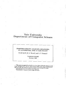
4.3 Routing Reconfiguration with MPLS-ff and Label Stacking With MPLS-ff support, we implement resilient routing reconfiguration. In our implementation, a central server performs precomputation of protection routing p, establishes labels for each protected link, signals of MPLS-ff setup, and distributes p. The central server can be integrated with Routing Control Platform [11] or Path Computation Element (PCE) [10]. Online reconfiguration is distributed, and conducted by each router locally. It has three components: failure detection and notification, failure response, and protection routing update. Below we go over each component. Failure detection and notification: We detect link failure using layer 2 interface monitoring. Upon a local failure event, a notification is generated and flooded to all other routers in the network through ICMP packets with type 42. In operational networks, failure detection and notification can be made more efficient using the deployed network management infrastructure. For example, SRLG failure can be detected by a risk modeling algorithm based on network monitoring [25]. The detection could be conservative (e.g., if any link in a SRLG is down, assume all links in the SRLG are down). Also, the operator can issue preparation notifications to all routers before starting a MLG maintenance operation. Failure response: After a failure is detected, MPLS-ff for the detected failure is activated by label stacking. Figure 2 is a simple example illustrating the failure response. An IP packet of flow (S1,D1) reaches router R1. R1 looks up the packet using the base forwarding table and decides that the nexthop for this packet is R2. Normally, the packet follows the base routing and is sent to R2.
Figure 2: Failure response example: (a) normal - R1 routes flows to R3 through R2; (b) link (R1,R2) fails - R4 and R5 carrying protection traffic by label stacking. If link (R1,R2) fails, R1 activates the protection routing for (R1,R2), looks up the protection label 200 for link (R1,R2) in ILM, and pushes label 200 onto the MPLS stack of the packet. The lookup in ILM indicates that the next-hop neighbor is R4, so R1 forwards the packet to R4. When the packet reaches router R4, R4 looks up the ILM for the incoming label 200. For the protection label 200, R4 has two NHLFEs: 40% of the flows to R2, and 60% to R5. For simplicity, we assume that the outgoing labels of the two NHLFEs are still 200; in practice the signaling may assign different labels. Assume that the hash of flow (S1,D1) on R4 selects R2, then R4 forwards the packet to R2. Similarly, protection traffic for flow (S2,D2) through R4 can be carried by R5. At R2, the protection label of the packet will be popped. The packet will be forwarded to R3 following the remaining base routing of OD pair (R1,R3). When the network recovers from a failure event, the base routing is immediately re-activated and the protection routing is disabled. Protection routing update: After a failure, each router needs to update the protection routing (i.e., reconfiguring next-hop splitting ratios) for other protected links. To facilitate local update, each router stores p in its RIB (routing information base). The storage requirement is O(|E|2 ). Considering that backbone routers already maintain the network topology information (e.g., in Link State Database), this additional storage overhead is acceptable. Due to the order independence of rescaling, when multiple failures happen, different routers can perform rescaling on their local copies of p. When all routers are notified of all failures, the routers will have a consistent protection routing p. During the transition process, different routers may have inconsistent p, which may lead to transient loops. If transient loops are of concern, techniques such as failure-carry packets (FCP) [26] can be integrated with R3.
5.
EVALUATIONS
We now evaluate R3 using both real experiments and extensive simulations based on realistic network topologies and traffic traces.
5.1
Evaluation Methodology
Network topology: For simulations, we use the PoP-level topology of a large tier-1 ISP network, called US-ISP. In addition, we use PoP-level topologies of three IP networks, Level-3, SBC, and UUNet (2003), as inferred by Rocketfuel [35]. We recursively merge the leaf nodes of the topologies with their parents until no nodes have degree one so that we have the backbone of the networks. We use OC192 as the capacity for links in the Rocketfuel topologies. We also generate a large backbone topology using GTITM. For our experimental results, we create the Abilene backbone topology (2006) on Emulab [41]. We scale down the link capacities
# Nodes 11 17 19 47 100 -
12
# D-Links 28 72 70 336 460 -
Table 1: Summary of network topologies used. to be 100 Mbps, and configure link delays to be measured values. Table 1 summarizes the used topologies. The data for US-ISP are not shown due to privacy concerns. Traffic: We obtained real hourly traffic demand matrices of USISP for a one-week period. For Rocketfuel topologies, we use the gravity model [45] described in [30] to generate synthetic traffic demands. To generate realistic traffic during our experiments on Emulab, we extract Abilene traffic matrix from measurement data and scale down the values. Then we generate traffic for each OD pair at the rate encoded in the traffic matrix. We use CAIDA Anonymized 2008 Internet traces [7] for real-time IP packet generation. Failure scenarios: To evaluate the performance under failures, we enumerate all possible single- and two-link failures, and randomly sample around 1100 scenarios of three- and four-link failures. We use random sampling for three- and four-link failures due to the large number of all possible such failures. This sampling is only needed for quantifying the performance under failures and not required for computing protection routing, since R3 does not require enumeration of failure scenarios. In addition, for US-ISP, we obtain real maintenance link groups (i.e., the sets of links that were under maintenance together) for a 6-month period, and treat each maintenance link group as a single failure event. Performance metrics: For simulation results, we use two performance metrics in our simulations: (1) bottleneck traffic intensity, and (2) performance ratio. Bottleneck traffic intensity measures network congestion. The performance ratio of an algorithm is defined as the ratio between the bottleneck traffic intensity of the algorithm and that of optimal flow-based routing, under the same network topology and traffic demand, and measures how far the algorithm is from being optimal under the given network topology and traffic demand. It is always no less than 1, and a higher value indicates that the performance of the algorithm is farther away from the optimal. We further evaluate the router storage overhead and the efficiency of resilient routing reconfiguration using measurement data using Emulab experiments. Algorithms: We consider the following base routing schemes: • OSPF: This is widely used in IP/MPLS networks for traffic engineering. For US-ISP, we use the IGP weight optimization technique in [13] and compute a set of optimized weights for each day during the evaluation period based on the 24 traffic demand matrices of that day. • MPLS-ff: The base routing is computed using the algorithms in Section 3. We consider the following protection algorithms. • CSPF-detour: This algorithm is widely used in fast rerouting. The bypass routing for a set of failed links is computed using OSPF algorithm with the failed links removed. The implementation of the bypass routing is generally based on standard MPLS. • OSPF reconvergence (recon): In this algorithm, the OSPF routing protocol is allowed to re-compute routing for every changed topology. • Failure-Carrying Packet (FCP): This is the algorithm as described in [26]. In this algorithm, individual data packet keeps track of topology changes that have been encountered by the packet, and the packet is routed along the OSPF path in the current snapshot of topology. • Path Splicing (PathSplice): This algorithm is proposed in [29].
OSPF+CSPF-detour OSPF+recon FCP PathSplice OSPF+R3 OSPF+opt MPLS-ff+R3 optimal
10 NormalizedMLU
Aggregation level router-level PoP-level PoP-level PoP-level router-level PoP-level
8 6 4 2 40
45
50
55
60
Interval
Figure 3: Time series of worst-case normalized traffic intensity with one failure during a given day for US-ISP. 7
OSPF+CSPF-detour OSPF+recon FCP PathSplice OSPF+R3 OSPF+opt MPLS-ff+R3
6 Performanceratio
Network Abilene Level-3 SBC UUNet Generated US-ISP
5 4 3 2 1 0
20
40 60 80 100 120 140 Scenariossortedbyperformanceratio
160
180
Figure 4: Summary of one failure: US-ISP. In our evaluation, we compute k = 10 slices with a = 0, b = 3 and W eight(a, b, i, j) = (degree(i)+degree(j))/degreemax , where degreemax is the maximal node degree of the network. When forwarding traffic, if a router detects that the outgoing link for a destination is unavailable, it detours traffic to this destination through other connected slices using uniform splitting. • R3: The protection routing is computed using the algorithms in Section 3. • Flow-based optimal link detour routing (opt): This is the optimal link detour routing for each given traffic and failure scenario. Specifically, for each failure scenario f , this scheme computes an optimal protection plan (i.e., a rerouting for each link in f ). Since the detour routing varies according to each failure scenario, it is challenging to implement in a practical way. Its performance is used to bound the best performance that can be possibly achieved by any practical protection algorithms.
5.2
Simulation Results
US-ISP: To preserve confidentiality of US-ISP, we do not report the absolute traffic intensity on the bottleneck link. Instead, we report normalized bottleneck traffic intensity. Specifically, for each interval in the trace, we compute the bottleneck traffic intensity using optimal flow-based routing when there is no failure. We then normalize the traffic intensity during different intervals by the highest bottleneck traffic intensity observed in the trace. Single failure: We first introduce one failure event (SRLG or MLG). At each interval, we assume that the network topology deviates from the base topology by only one failure event. We identify the worst case performance upon all possible single failure events, and report normalized traffic intensity on the bottleneck link. Figure 3 shows the results. For clarity, we zoom in to a one-day time frame during the evaluation period; thus, there are 24 intervals. We make the following observations. First, R3 based protection (MPLSff+R3 and OSPF+R3) performs close to the optimal, and achieves performance similar to flow-based optimal link detour routing on top of OSPF (OSPF+opt). However, flow-based optimal link detour (opt) requires the computation of optimal protection routing for each individual topology-change scenario, whereas R3 achieves similar performance with only a single protection routing and a simple, light-weight routing reconfiguration. Second, comparing the two R3 schemes, we observe that MPLS-ff+R3 performs better than OSPF+R3 (see intervals 40 to 48). This is expected since OSPF is less flexible than MPLS. Third, without a good protection
4
OSPF+CSPF-detour OSPF+recon FCP PathSplice OSPF+R3 OSPF+opt MPLS-ff+R3
3 2.5
OSPF+CSPF-detour OSPF+recon FCP PathSplice OSPF+R3 OSPF+opt MPLS-ff+R3
2.4 Performanceratio
Performanceratio
3.5
2 1.5
2.2 2 1.8 1.6 1.4 1.2
1
1 0
200
400
600
800
1000
1200
0
Scenariossortedbyperformanceratio
100
2.5
Performanceratio
Performanceratio
3
400
500
600
OSPF+CSPF-detour OSPF+recon FCP PathSplice OSPF+R3 OSPF+opt MPLS-ff+R3
2.4
OSPF+CSPF-detour OSPF+recon FCP PathSplice OSPF+R3 OSPF+opt MPLS-ff+R3
3.5
300
(a) two failures
(a) two failures 4
200
Scenariossortedbyperformanceratio
2
2.2 2 1.8 1.6 1.4 1.2
1.5
1
1 0
200
400
600
800
1000
0
1200
Scenariossortedbyperformanceratio
(b) sampled three failures Figure 5: Sorted performance ratio under multiple failures during peak hour: US-ISP.
200
400
600
800
1000
1200
Scenariossortedbyperformanceratio
(b) sampled three failures Figure 6: Sorted performance ratio: SBC. 2.2 Performanceratio
2
OSPF+CSPF-detour OSPF+recon FCP PathSplice OSPF+R3 OSPF+opt MPLS-ff+R3
Performanceratio
scheme, OSPF+recon, OSPF+CSPF-detour, and FCP all lead to 1.8 higher levels of normalized traffic intensity. In the early part of the 1.6 day, their traffic intensity can be as high as 3 times that of the other routing protection schemes (∼5 vs. ∼1.5). Fourth, starting from 1.4 interval number 49, FCP starts to have better performance than 1.2 OSPF+recon, OSPF+CSPF-detour. But its traffic intensity in the 1 later part of the day can still be as high as 2 times (e.g., during in0 100 200 300 400 500 600 700 terval number 60) that of MPLS-ff+R3, OSPF+R3 and OSPF+opt. Scenariossortedbyperformanceratio Finally, by rerouting traffic to multiple slices in a “best effort” fash(a) two failures ion, PathSplice leads to less congestion and achieves much better OSPF+CSPF-detour 2.2 performance than other existing protection algorithms, though it is OSPF+recon still less efficient than R3 based algorithms. FCP 2 PathSplice The previous evaluation shows the effectiveness of R3 during OSPF+R3 1.8 one day. Next, we summarize the overall performance during the OSPF+opt 1.6 MPLS-ff+R3 entire evaluation period (which lasts seven days). Figure 4 shows 1.4 the performance ratio versus the time interval sorted based on the performance ratio. We make the following observations. First, 1.2 MPLS-ff+R3, OSPF+R3, and OSPF+opt consistently perform within 1 30% of the optimal throughout the entire evaluation period. Sec0 200 400 600 800 1000 1200 ond, OSPF+recon, OSPF+CSPF-detour, PathSplice, and FCP all Scenariossortedbyperformanceratio cause significant performance penalty. The performance of OSPF+recon, (b) sampled three failures OSPF+CSPF-detour, and FCP can be 260% higher than optimal. Figure 7: Sorted performance ratio: Level 3. PathSplice performs better, but it still can be 100% higher than the FCP, and PathSplice reach at least 2.4 times of optimal, while MPLSoptimal while R3 based schemes are within 30%. Thus, the traffic ff+R3 and OSPF+R3 reach only 1.6; thus they are at least 50% intensity of PathSplicing can be 54% higher than R3. higher than R3 based protection. Multiple failure events: Next we evaluate using multiple failure Summary: For US-ISP, R3 based schemes consistently achieve betevents in US-ISP. For clarity of presentation, we fix the interval (a ter performance than OSPF+recon, OSPF+CSPF-detour, FCP, and peak hour) and evaluate the failure events. We report results for PathSplice, outperforming them by at least 50% in all scenarios and two failures and sampled three failures. We report only sampled much higher in some scenarios. three failures because there are too many failure scenarios to enumerate; thus, we use random sampling. Figure 5 shows the perforRocketfuel topologies: Next we evaluate using Rocketfuel topolomance ratio versus the scenario sorted based on the performance gies. For each Rocketfuel topology, we randomly generate one trafratio. To make it easier to read, we have truncated the y-axis of fic matrix using gravity model. Due to lack of SRLG information, Figure 5 at the value of 4. We observe that under two and three we generate all two-link failures and randomly sample around 1100 failures, MPLS-ff+R3 and OSPF+R3 continue to significantly outthree-link failures. We then evaluate the performance of different perform OSPF+recon, OSPF+CSPF-detour, FCP, and PathSplice. algorithms under these failures. From Figure 5(a), we observe that OSPF+recon, OSPF+CSPF-detour, Figure 6 and Figure 7 show the performance ratios for SBC and FCP and PathSplice can cause bottleneck traffic intensity to be Level 3, respectively. We choose these two topologies as they more than 3.7 times of the optimal for two failures. This is 94% give representative results among the Rocketfuel topologies. From higher than the highest of MPLS-ff+R3 and OSPF+R3 (they reach these figures, we make the following observations. First, on SBC, around 1.9). For three failures, OSPF+recon, OSPF+CSPF-detour, MPLS-ff+R3, which jointly optimizes base routing and protection
Penalty envelope: Our R3 formulation introduces a penalty envelope on normal case MLU. The goal is to balance between being robust to topology changes and being optimal when there are no topology changes. We demonstrate the importance of this technique by evaluating network performance under no topology changes. In Figure 9, we show the performance of four algorithms: R3 without penalty envelope, OSPF, R3 with penalty envelope, and optimal. We pick a time period when OSPF performs particularly well with optimized IGP weights. We make the following observations. First, adding the penalty envelope significantly improves normal case performance. The 10% penalty envelope is effective and R3 performs within the envelope during normal operations. Second, R3 without penalty envelope can lead to significant performance penalty in normal cases. Its normalized traffic intensity sometimes goes as high as 200% of the optimal and may perform even worse than OSPF. The reason is that R3 without penalty envelope optimizes exclusively for the performance under failures and only enforces no congestion during normal network topology and traffic. Robustness on base routing: The previous evaluation shows that
R3noPE OSPF R3 optimal
NormalizedMLU
2 1.5 1 0.5 0
20
40
60
80
100
120
140
160
Interval
Figure 9: Time series of normalized traffic intensity with no change during a week for US-ISP. NormalizedMLU
Prioritized R3: We evaluate prioritized R3 using three classes of traffic with different priorities. Specifically, we extract traffic of TPRT and TPP from the US-ISP backbone traffic in a peak interval. For confidentiality, we rescale the traffic volumes of TPRT and TPP. We then subtract these two types of traffic from the total traffic and treat the remaining traffic as IP. For prioritized R3, we set the protection levels of TPRT, TPP, and IP to four failures, two failures, and one failure, respectively. For general R3, all traffic is protected against one failure. We report results for all single failures, top 100 worst-case two-failure scenarios, and top 100 worst-case fourfailure scenarios out of the sampled four failures. Figure 8 shows the normalized bottleneck traffic intensities for the three classes of traffic under R3 with and without priority. We make the following observations. First, both prioritized and general R3 provide congestion-free rerouting under single failures. Comparing the performance between prioritized and general R3, we observe that IP traffic has lower bottleneck traffic intensity under prioritized R3 than under general R3, while the bottleneck traffic intensities of TPP and TPRT under prioritized R3 are slightly higher than under general R3. The reason for the latter is because even though IP traffic has lower priority than TPP and TPRT under multiple failures, prioritized R3 can give IP better treatment under single failures as long as TPP and TPRT traffic are well protected, which is the case (i.e., the bottleneck traffic intensities of TPP and TPRT are always smaller than 0.4 under single failures). Second, under two-link failures, prioritized R3 guarantees no congestion for TPRT and TPP, whereas TPRT and TPP experience congestion under general R3. The bottleneck traffic intensities of IP traffic are higher under prioritized R3 than under general R3, which is inevitable due to limit of resources. Third, under four-link failures, TPRT incurs no congestion using prioritized R3, whereas all traffic experiences congestion using general R3. Even TPP, which is protected up to two-link failures, achieves lower traffic intensities under prioritized R3 than under general R3. As expected, IP traffic experiences congestion under both general and prioritized R3 during four-link failures. These results demonstrate that prioritized R3 is effective in providing differentiation to different classes of traffic.
3 2.5
2.2 2.1 2 1.9 1.8 1.7 1.6 1.5 1.4 1.3
OSPFInvCap+R3 OSPF+R3
0
5
10 15 20 25 30 35 40 ScenariossortedbynormalizedMLU
45
50
(a) one failure 4.5
OSPFInvCap+R3 OSPF+R3
4 NormalizedMLU
routing, significantly out-performs all OSPF based algorithms, including OSPF+opt. This demonstrates the advantage of joint optimization of base routing and protection routing. Second, on Level 3, MPLS-ff+R3 and OSPF+R3 have very similar performance, and consistently out-perform other OSPF based algorithms, except for OSPF+opt. In fact, on Level 3, OSPF+opt performs very close to optimal and slightly better than MPLS-ff+R3 and OSPF+R3. Recall that it is substantially more expensive to implement OSPF+opt, this indicates that on networks with very good OSPF routing, R3 on top of OSPF can be used to achieve most of the gains of R3 while retaining the simplicity of OSPF routing.
3.5 3 2.5 2 1.5 1 0
200 400 600 800 1000 ScenariossortedbynormalizedMLU
1200
(b) two failures Figure 10: Sorted normalized traffic intensity: US-ISP during peak hour. R3, which jointly optimizes base routing and protection routing, out-performs OSPF+R3. So a better base routing leads to better overall performance. To further understand the impact of base routing, we conduct the following evaluation. We compare two versions of OSPF as base routing: (i) OSPFInvCap+R3 and (ii) OSPF+R3, where in the former the IGP weights of the base routing is inverse proportional to link capacity and in the latter IGP weights are optimized. As shown in Figure 10, R3 based on OSPFInvCap is significantly worse than R3 based on an optimized OSPF routing. These results further demonstrates the importance of base routing.
5.3
Implementation Results
We implement R3 on Linux and evaluate its efficiency. Offline computation complexity: We first evaluate the computation complexity of R3. We run R3 offline precomputation for the 6 topologies with different failure guarantees. All computation is done using a single Linux machine with commodity hardware configuration (2.33 GHz CPU, 4 GB memory). We employ ILOG CPLEX 10.0 [8] as the linear program solver. Table 2 summarizes the results. We observe that the precomputation time fluctuates with the number of failures and is typically below half an hour. This is because the complexity of the linear program (7) is independent of the number of failures. In contrast, explicit enumeration of failure scenarios can quickly become prohibitive as the number of failures increases. Storage and MPLS overhead: One concern about R3 protection implementation based on MPLS-ff is router storage overhead (i.e., FIB and RIB size), given that routers need to maintain the protection labels for all protected links and store local copies of the protection routing p. To evaluate the storage overhead, for a given topology, we run R3 MPLS-ff protection assuming that all backbone links are protected
1.2 1 0.8 0.6 0.4 0.2 0 0
5 10 15 20 25 30 35 40 Scenariossortedbynormalizedbottleneckintensity
Normalizedbottleneckintensity
Normalizedbottleneckintensity
Normalizedbottleneckintensity
IP(generalR3) IP(R3withpriority) TPP(generalR3) TPP(R3withpriority) TPRT(generalR3) TPRT(R3withpriority)
1.4
1.4 1.2 1 0.8 0.6 0.4 0.2 0
45
0
10 20 30 40 50 60 70 80 90 Scenariossortedbynormalizedbottleneckintensity
1.4 1.2 1 0.8 0.6 0.4 0.2 0 0
100
10
20
30
40
50
60
70
80
90 100
Scenariossortedbynormalizedbottleneckintensity
0.5
normalcase 1linkfailure 2linkfailures 3linkfailures
0.3%
normalcase 1linkfailure 2linkfailures 3linkfailures
0.4
Averagelossrate
0.09 0.08 0.07 0.06 0.05 0.04 0.03 0.02 0.01 0
Normalizedtrafficintensity
Normalizedthroughput
(a) 1-link failures (b) worst-case scenarios of 2-link failures (c) worst-case scenarios of 4-link failures Figure 8: Sorted bottleneck traffic intensity for prioritized traffic: US-ISP (note that the legend is the same for all three plots).
0.3 0.2 0.1
normalcase 1linkfailure 2linkfailures 3linkfailures
0.2%
0.1%
0 0
10
20
30
40
50
60
70
80
0
ODpairindexsortedbynormalcasenormalizedthroughput
5
10
15
20
25
0
2
4
D-Linkindexsortedbynormalcasenormalizedtrafficintensity
6
8
10
Egressrouterindex
(a) normalized throughput (b) normalized link load (c) aggregated loss rate at egress routers Figure 11: Network performance using R3 under multiple link failures. 1 0.3 1.80 1.46 1010 1388 21.3
2 0.30 1.97 1.76 572 929 21.9
3 0.30 2.56 1.75 1067 1971 21.4
4 0.32 2.71 1.76 810 2001 20.1
5 0.33 2.46 1.92 864 1675 22.1
6 0.29 2.43 1.91 720 2131 21.8
RTT(milisecond)
Network/# failures Abilene Level-3 SBC UUNet Generated US-ISP
Table 2: R3 offline precomputation time (seconds). # ILM 28 72 70 336 460 -
# NHLFE 71 304 257 2402 2116 -
FIB memory