Random Finite Set-based Bayesian Filters Using Magnitude-adaptive Target Birth Intensity Tiancheng Li, Shudong Sun School of Mechanical Engineering Northwestern Polytechnical University Xi’an, 710072, China
[email protected];-
Juan Manuel Corchado
Ming Fei Siyau
BISITE group, School of Science University of Salamanca Salamanca, 37008, Spain
[email protected]
School of Engineering & Design London South Bank University London, SE1 0AA, UK
[email protected]
Abstract—Modelling new-born targets that spontaneously appear in the multi-target tracking scene is an indispensable yet challenging task for any multi-target tracker, which asks for a careful formulation of the target birth intensity (TBI) in random finite set based Bayesian filters. However, the TBI is widely assumed to hold for a constant magnitude that needs to be specified in advance, indicating a constant speculation for the number of new targets to be appeared at all scans. This is not always desirable and can be problematic as the TBI magnitude is generally unknown and varies in time. In this paper, a data-driven approach is proposed to determine the TBI magnitude in real time based on the information contained in the newest observations. Simulations of the sequential Monte Carlo implementation of the probability hypothesis density filter and the multi-Bernoulli filter have demonstrated the validity of our approach. Keywords—Multi-target tracking; random finite set; PHD filter; multi-Bernoulli filter; particle filter
I. INTRODUCTION Multi-target tracking (MTT) refers to online estimating the states of multiple moving targets in the presence of spontaneous appearance/disappearance of targets, which has a variety of applications in both military and commercial realms. Far more complex than just a juvenile sense of single-target tracking, the challenges in MTT consist of at least four parts: 1) The number of targets is both unknown and time-varying due to the spontaneous appearance and disappearance of targets; 2) Clutter exists and can be significant; 3) Targets can be miss-detected; and 4) The states and observations of targets collected are finite-set-valued random variables that are random in both the number of elements and the values of the elements. The idea of modelling the states of targets and observations as random finite sets (RFS) together with the point process theory have been proven to be concise and adequate to formulate the challenging MTT problem. Based on the finite set statistics, the probability hypothesis density (PHD) filter [1] (and its higher order form: cardinalized PHD (CPHD) filter [2]) and the multi-Bernoulli filter [3, 4] afford two efficient solutions which have attracted increasing attentions. As a key prerequisite of tracking, environment formulation is required for setting up close-to-truth models regarding targets (including the target birth function [5, 6] and unknown target [19]) and observations (including detection uncertainty [7], imprecise observation and non-standard observation [4], and clutter [7]). Knowledge of these profile elements are of This work is sponsored by Excellent Doctorate Foundation of NPU and National Natural Science Foundation of China (No.51075337; No. 71271170).
critical necessity and significance in the RFS-based Bayesian filters including the PHD filter and the multi-Bernoulli filter. This paper focuses on modelling new-birth targets for the RFS-based Bayesian filter. ‘Birth’ is a classical model in the theory of branching processes [8]. Generally, the target birth model is indispensable to any multi-target tracker and has to be applied at each filtering step, which corresponds to a target birth intensity (TBI) item in the propagation equations of RFS-based Bayesian filters. The goal of modelling the TBI is to capture the newly appearing targets online, integrating them into the underlying multi-target density and allowing the consequent ‘tracking’. Nevertheless, information about the birth of new targets is often very limited due to the spontaneity of target birth, rendering the problem very challenging. Basically, two critical issues are involved with TBI modeling. One is the birth function (birth area and model) of new targets, which is the main part of TBI. The other is the number of new targets to appear (or the appearing probability of one target) that is modelled as the magnitude of TBI. For the birth area of new targets, a typical case is that it is known a priori. For example, targets appear around the fixed area such as airports [9] or most likely from the edges of the field of view [10]. In these cases, the appearance area of new-birth targets can be built efficiently by using the known profile. In more common cases, where the targets can appear anywhere, it will require to cover the entire state space. To overcome this computational inefficiency, observation-driven birth intensities were independently proposed in [5, 11] and [17] to improve tracking performance as well as to obviate exact knowledge of the birth intensity for the particle filter implementation and for the GM implementation of the PHD filter. The idea has been extended to the Cardinality Balanced Multi-target Multi-Bernoulli (CBMeMBer) filter [15]. In the SMC implementation, new particles are positioned around observations to represent newborn targets. In the closed-form implementation, observations are classified into two parts that correspond to newborn targets and survival targets respectively in [12, 13] and a detector based on the continuity of observations was used to generate intensities of new targets. Furthermore, Doppler information might be useful to initialize a more realistic target/track velocity [14]. All of these works show that observation is useful for system parameter setting. In contrast, lesser works have been devoted to adapting the magnitude of TBI. Previous works as aforementioned proposed adaptive target birth functions, yet offered little clue about how the TBI magnitude is determined. In current studies, the TBI is
manually assigned with a constant magnitude, i.e. a blind and fixed speculation of the number of targets is applied. This can be problematic as it is often unclear how to specify the TBI magnitude offline, let alone the TBI magnitude varies in time. This paper proposes a data-driven mechanism to adapt the TBI magnitude by using the newest observations in the RFS-based Bayesian filter. An earlier version of the idea is given in [20] with its application on SMC-PHD filter. To narrow the scope of the illustration, this paper primarily investigates the case of the SMC implementation of the PHD filter and the CBMeMBer filter, which are two typical RFS-based Bayesian filters. A brief summary of the idea of SMC-PHD/Multi-Bernoulli filters and the TBI modeling problem is given in section II. The observation-driven online TBI magnitude adaptation approach is presented in section III. Simulation is given in section IV and the conclusion in section V. II. BACKGROUND AND PROBLEM STATEMENT A. RFS formulation of multi-target tracking In order to model the MTT problem, let define the and define the space of finite subsets of targets . Suppose that space of finite subsets of observations at time , the collections of the states of targets are a RFS where is the number of targets, and , ,…, , the observations are a RFS , ,…, , is the number of observations. where at time 1 , each Given a multi-target state either continues to exist at time with survival and to move to a new state with a probability , | or dies with transition probability density | probability 1 . At time , a given target is , and either detected with detection probability , generates an observation with likelihood | or miss-detected with probability 1 . We have ,
X k = ( U Sk k −1 ( x))( U Bk k −1 (x)) ∪ Rk x∈Xk −1
x∈Xk −1
(1)
and | are the RFS of targets that where | , and is survive and spawn at scan from target states the RFS of targets that appear spontaneously at scan .
Zk = ( U Gk ( x)) ∪ Ck x∈Xk
(2)
where is the random set of observations of target is the set of clutter observations at scan . and Let | and | be the multi-target posterior and the | : , multi-target prior, namely | | | | , where , … . The Bayesian | : : RFS filter evolves in time via the following recursions
... → π k −1 k −1 → π k k −1 → π k k → ... which consists of two basic steps: prediction and update. B. The PHD filter General multi-target trackers as well as the basic RFS-based filter require the following assumptions:
(A.1) Each target is assumed to evolve and generate observations independently of others; (A.2) The clutter distribution is assumed to be Poisson and independent of the observations; (A.3) One target is assumed to generate no more than one observation at each scan; In addition, the PHD filter assumes that (A.4 Poisson): Target birth is assumed to be Poisson [16]. Proposition 1 (PHD Prediction) the time-update step is
π k k −1 ( x) = ∫ φk k −1 ( x u)π k −1 k −1 (u)du + γ k ( x)
(3)
χ
where the following abbreviation is used
φk k −1 ( x u) = pS ,k (u) f k k −1 ( x u) + bk ( x u) | denotes the intensity function of the RFS of targets spawned from the previous state , and is the birth intensity function of new targets at scan k. The TBI may be integrated into the PHD updater [17] rather than integrated into the predictor as above. where |
Proposition 2 (PHD Update) the data-update step is ⎡
π k k ( x ) = ⎢ (1 − p D , k ( x )) + ⎣
where
pD ,k ( x ) g k ( z x ) ⎤ ( x ) (4) ⎥π κ k ( z ) + C k ( z ) ⎦ k k −1
∑
z∈Z k
is the clutter intensity at time Ck ( z ) = ∫ pD , k (u ) g k ( z u )π k k −1 (u )du
(5)
To note, the clutter intensity function can be slimmed down due to gating of clutter [23]. C. The multi-Bernoulli filter Contrary to the classical PHD filter, the forth assumption required by the CBMeMBer filter is that (A.4 Bernoulli): Target birth is multi-Bernoulli, while assumptions (A.1-3) still hold. Different assumptions derive different equations of the PHD filter and the CBMeMBer filter; see [3]. The multi-target Multi-Bernoulli (MeMBer) filter that was proposed by Mahler [3] and partly corrected by Vo [4], approximates the Multi-target Bayes recursions by using multi-Bernoulli RFSs. To be consistent with the previous ·| : denotes the multi-target posterior denotation, density at time . The corrected MeMBer filter as called Cardinality Balanced MeMBer filter can be summarized as in the following two propositions: Proposition 3 (MeMBer Prediction) if at time 1 , the posterior multi-target density is a multi-Bernoulli of the form:
{
}
π k −1 = ( rk(−i )1 , pk(i−)1 )
M k −1
Then, the predicted multi-target multi-Bernoulli and is given by
{
}
π k |k −1 = ( rP(i, k) |k −1 , pP(i,)k | k −1 ) where
M k −1
i =1
(6)
i =1
density
{
is
}
∪ ( rΓ(,ik) , pΓ(i,)k )
M Γ ,k
i =1
also
a (7)
rP( i, k) |k −1 = rk(−i )1 pk( i−)1 , pS , k
(8)
f k |k −1 ( x | ⋅), pk(i−)1 pS , k
pP(i,)k |k −1 =
(9)
pk( i−)1 , pS , k
f k |k −1 (⋅ | ζ ) : single target transition density at time k , given previous state ζ pS , k (ζ ) : probability of target existence at time k , given state ζ
{( r
(i ) Γ,k
}
, pΓ(i,)k )
M Γ ,k
i =1
: parameter of the multi-Bernoulli
RFS of births at time k Proposition 4 (Cardinality balanced MeMBer Update) if at time , the predicted multi-target density is a multi-Bernoulli of the form
{
}
π k|k −1 = ( rk(|ik)−1 , pk(i|k) −1 )
M k|k −1
(10)
i =1
then, the posterior multi-target density can be approximated by a multi-Bernoulli with unbiased cardinality as follows:
{
}
π k = ( rL(,ik) |k −1 , pL(i,)k |k −1 )
M k|k −1
i =1
{
}
∪ ( rU( z, k) , pU( z,)k )
z∈Zk
(11)
where
rL(,ik) = rk(|ik)−1
1 − pk(i|k) −1 , pD, k
pL( i,)k |k −1 ( x) = pk( i|k) −1 ( x) M k |k −1
∑
(z) U ,k
r
=
i =1
pk(i|k) −1 , pD, k
M k|k −1
rk(|ik)−1 pk(i|k) −1 ,ψ k , z
(i ) k | k −1
∑ 1− r
M k|k −1
( x) =
1 − pk( i|k) −1 , pD , k
(1 − r
(i ) k | k −1
i =1
p
1 − pD , k ( x)
(13)
rk(|ik)−1 (1 − rk(|ik)−1 ) pk(i|k) −1 ,ψ k , z
κ k ( z) +
(z) U ,k
(12)
1 − rk(|ik)−1 pk( i|k) −1 , pD , k
rk(|ik)−1
∑ 1− r i =1
M k|k −1
∑ 1− r i =1
2
(14)
pk(i|k) −1 , pD , k
( x)ψ k , z ( x)
(i ) k | k −1 (i ) k |k −1 (i ) k | k −1 (i ) k | k −1 (i ) k |k −1
r
)
p
p
(15)
conditions that specify the initial distributions of the numbers of targets and clutter [8]. Furthermore, amplitude information and Doppler information of the observation can be further considered to provide initial target velocities [18]. In contrast, the magnitude of TBI has not attracted sufficient is widely applied with a constant attention as e.g. 20% [9, 23], 20% (10% each in two regions) magnitude [18], 5% [24], 25% [5], 10% and 1% [17] (separately in two regions) and 2%, 3%, 2% and 3% (separately in four regions) [4]. That is, in the SMC implementation, the same number of new particles of a fixed weight mass are generated at each scan. This ad-hoc approach for determining the magnitude of TBI is not always desirable and can be problematic. If given the knowledge that new targets are more likely to be born at special steps, the magnitude of TBI should be large. Otherwise, it should be small or even naught. To employ a magnitude that matches the background is strongly required to build a realistic TBI model. Based on this, we propose an observation-driven method that adapts the magnitude of TBI by using the newest observations, called magnitude-adaptive TBI. It is worth noting that the proposed approach is not specific to any . particular The PHD recursions can be approximately implemented via particles [9] or finite GM (Gaussian mixture) [18], as can the CBMeMBer equations [4]. Specifically, the particle filter that uses a set of weighted samples to approximate the density distribution of interest is a powerful statistical method that is free of linearity and Gaussian assumption and is thereby able to meet general MTT requirements. A key difference between them is that all particles belong to the same joint distribution and so are treated the same in the SMC-PHD filter while they belong to different Bernoulli, and should be handled separately in the SMC-CBMeMBer filter. As such, the weights of particles are correlated with each other in the SMC-PHD filter while the weight of particles of different Bernoulli distributions are independent of each other (only the one in the same set are correlated) in the SMC-CBMeMBer filter. For each target birth model, the TBI magnitude is represented as the weight mass of new particles in the former while it is the model parameter , in the latter. This difference will produce a slight difference of calculation in the implementation of our approach.
,ψ k , z
where ψ k , z ( x ) = g k ( z | x ) p D , k ( x )
D. Modeling of TBI In the PHD/CBMeMBer filter, the birth target density can where indicates be written as models the magnitude and different TBI model, the birth function. and correspond to two reflects critical issues that need to be considered separately. the average number of new targets and provides is information of target birth area and function. addressed to be observation-driven target birth position/function [5, 11-13], uniform birth function [21], or entropy distribution [22] etc. Mathematically, the target birth and death problem was formulated for arbitrary boundary
III. MAGNITUDE-ADAPTIVE TBI Standard implementations of the SMC-PHD filter and the SMC-CBMeMBer filter can be found in [9, 4]. In this section, we will first present the magnitude-adaptive TBI methodology for the SMC-PHD filter and then discuss its implementation in the SMC-CBMeMBer filter. A. Methodology: Adapting TBI in the SMC-PHD filter Since the target birth is spontaneous, the assumption that new targets may appear at any step must still be applied. Proposition 5 (Tentative TBI Magnitude) A tentative TBI is assumed with magnitude ̃ e.g. ̃ 0.2 for each step. As common a fixed number of particles are used for each target.
That is,
̃
new particles
,
,…,
(as
called new-born particles) is assigned where the state of them is
determined according to a specified birth function the homogenous weight can be determined as ̃
while (16)
|
Then, traditional steps of the SMC-PHD prediction and updating can be processed as follows. Given the importance ·| , ·| and assuming that there are densities original particles in time step 1 and new-born particles are allocated for possible new-born targets as above. According to (3), the particle approximation of the PHD predictor (realizing Proposition 1) can be written as
π k k −1 ( xk ) =
Lk −1 + J k
∑ i =1
where
wk(ik) −1δ x ( i ) ( xk )
⎧⎪qk (⋅ xk(i−)1 , Z k ), i = 1,..., Lk −1 xk(i ) ~ ⎨ ⎪⎩ pk (⋅ Z k ), i = Lk −1 + 1,..., Lk −1 + J k φk k −1 ( xk( i ) xk(i−)1 ) wk( i−)1 wk( ik) −1 = , i = 1,..., Lk −1 qk ( xk( i ) xk(i−)1 , Z k ) wk( ik) −1 =
(17)
k
(18)
(19a)
γ k ( xk( i ) )
(19b) , i = Lk −1 + 1,..., Lk −1 + J k J k pk ( xk( i ) Z k ) The particle approximation of the PHD updater (realizing Proposition 2) is
π k k ( xk ) =
Lk −1 + J k
∑ i =1
where
wk( ik) δ x( i ) ( xk )
(20)
k
⎡ pD ,k ( xk(i ) ) g k ( z xk(i ) ) ⎤ (i ) ⎥w wk(ik) = ⎢1 − pD ,k ( xk(i ) ) + ∑ (21) κ k ( z ) + Ck ( z ) ⎥ k k −1 ⎢⎣ z∈Zk ⎦ Ck ( z ) =
Lk −1 + J k
∑ j =1
( j)
pD, k ( xk( j ) ) gk ( z x k )wk( jk)−1
(22)
The next step is to calculate the required TBI magnitude based on the assumed ̃ and the underlying observation . Proposition 6 (Confirmed TBI magnitude) Given the flow of (16) to (22), the updated weight mass of these new-born particles is Jk
rˆk = ∑ wk( ik)
(23)
i =1
which can be interpreted as an estimate of the average number of new targets in the assigned TBI region, i.e. a Bayesian estimate of the magnitude of TBI. However, the TBI magnitude might be overestimated via (23), since clutter can fall into the target birth area to pull up the weight of new-born particles; this is a drawback of the PHD filter where, the number of targets will be overestimated. In order to avoid the overshoot that a large value would be obtained from (23) due to dense clutter or existing targets, the magnitude can be further hard-limited to not exceed an upper (other remedy strategies might also work). Then, threshold the modified magnitude for the TBI is given as follows
̃
∑
|
,
(24)
Now that the required TBI magnitude can be obtained via (24). The next step is to incorporate the result into the filter to perform the formal filtering. One straightforward way is to update ̂ in (16) and then repeat all the calculations from (16) to (22), which consist of both the PHD predictor and updater. This will work without any problem but is computationally intensive. To save computation, calculations that have already been done (in the tentative stage to obtain the required ̂ ) can be used directly to avoid duplicated computation. Based on the obtained magnitude of TBI in (24), there are two possible ways as described in Proposition 7 and 8: Proposition 7 (Formal PHD Filtering) Based on (24), reproduce new-born particles to replace the tentative one and then re-process the calculation given in (19b) and (21~22). Proposition 8 (Formal PHD Filtering) Use the previous tentative particles but re-associate their weights as (16) based on (24) and recalculate (21~22). Remark 1 In Proposition 7, all calculations based on the original particles in (21~22), which take a large part of the computation for PHD updating, do not need to be repeated but instead, the results obtained in the tentative step can be directly used for formal PHD updating. Proposition 8 can save more computation as it does not need to re-generate new-born particles and update their states. What needs to be re-produced is the initialization of the weight of these particles according to the estimated magnitude of TBI. In this case, only very few calculations related to the weight of new-born particles i.e. Eq. (19b) and (21) need to be redone at the formal filtering stage. Specifically, the following computationally intensive part of (21) does not need to be recalculated.
⎡ pD , k ( xk(i ) ) g k ( z xk(i ) ) ⎤ (i ) ⎢1 − pD , k ( xk ) + ∑ ⎥ κ k ( z ) + Ck ( z ) ⎥ ⎢⎣ z∈Z k ⎦ B. Implementation with multiple TBI model In cases that new targets have multiple birth models e.g. new targets appearing at different areas; they need to be modelled as separate functions with individual magnitudes. In this case, the magnitude of each TBI function can be modelled separately as described in the single TBI model, which is independent of each other. This means, in each TBI model, an assumed number of tentative particles are used to process the tentative PHD updating independently without interaction. The estimated TBI magnitude shall be used separately in each TBI model. We call this the independency of the magnitude of the TBI. This will be demonstrated in our simulation. It is worth noting that, it will be still difficult to handle the case where different TBI functions are highly overlapped and hence their birth PHDs are highly correlated in close proximity. In this case, the calculation (23) is no longer straightforward or may even be inapplicable. Intuitively speaking, it is not straight to clearly distinguish whether a new target is generated by model A or by model B if they share a common target birth area (although sometimes it is unnecessary to do so). As our suggestion, the estimated TBI magnitude shall be shared proportionally between TBIs owning the common area.
C. Adapting TBI in the SMC-CBMeMBer filter The TBI magnitude parameter , , 1, … , , required by the CBMeMBer filter represents the probability of the underlying track that belongs to a new target and can be calculated online in a very similar way to the application in the SMC-PHD filter. The following Propositions 9-10 aim to obtain the required TBI magnitude and Proposition 11 states the formal SMC-CBMeMBer filtering. Predicting step (realizing Proposition 3): 1 the multi-Bernoulli posterior Suppose that at time multi-target density is given as (6) and each , 1, … , comprises a set of weighted particles
,
,
,
Suppose that at time the predicted multi-Bernoulli multi-target density | is given as (10) (where | , 1, … , | comprises a , ) and each |
(i ) k | k −1
p
p ( x) = M k |k −1
∑
k −1
Proposition 9 (Tentative CBMeMBer Filtering) Assume ̃ (a specified parameter) for the ith target birth model , of particles per target are used, i,e, and a fixed number
new-born particles
,
,
,
,
, ,…,
wΓ( i,,kj ) = wΓ( i,,kj ) /
L(Γi ,)k −1
∑ j =1
(i , j ) Γ,k Γ,k (i) (i, j ) k k Γ, k
p
(x
)
b (x
Then the multi-Bernoulli distribution
,
,
,
,
(7) is represented by these new-born particles, where parameter of interest and , is defined as rΓ( i,k)
pΓ( i,)k = ∑ wΓ( i,,kj )δ x ( i , j ) ( x )
,
p
L(ki−)1
∑w j =1
(i , j ) L,k
(i, j ) k −1
pS , k ( x
(i, j ) k −1
)
L(ki−)1
( x) =
(i ) L,k
=
(i ) M k|k −1 Lk|k −1
xP(i,,kj|)k −1 ∼ qk(i ) (⋅ | xk(i−,1j ) , Zk ), j = 1,..., L(ki−) 1 L(ki−)1
wP( i,,kj|)k −1 = wP( i,,kj|)k −1 / ∑ wP( i,,kj|)k −1
(30) (31)
j =1
wk( i−, 1j ) f k |k −1 ( xP( i,,kj|)k −1 | xk( i−, 1j ) ) p S , k ( xk( i−, 1j ) ) qk( i ) ( xP( i,,kj|)k −1 | xk( i−, 1j ) , Z k )
Updating step (realizing Proposition 4):
(32)
(35)
( z)
)
(36)
( z)
∑ ∑w
( z )δ x( i , j ) ( x)
(i , j ) U ,k
k |k −1
j =1
L(ki|k) −1
∑w
(i , j ) k | k −1
j =1
(i, j ) L,k
w
(37)
(i, j ) L,k
=w
(38)
p D , k ( xk( i|k, j−)1 ) L(ki|k) −1
∑w
/
(39)
(i, j ) L,k
j =1
wL(i,,kj ) = wk(i|k, j−)1 (1 − pD, k ( xk(i|k, j−)1 )) (i ) U ,k
(z) =
(i, j ) U ,k
w
L(ki|k) −1
∑w
(i , j ) U ,k
( z) = w
ψ k , z ( xk( i| k, j−)1 )
( z) /
wU( i ,, kj ) ( z ) = wk( i| k, j−)1
(40) (41)
(i, j ) k | k −1
(i) M k |k −1 Lk |k −1
∑ ∑w
( z)
(42)
ψ k , z ( xk( i| k, j−)1 )
(43)
i =1
rk(|ik)−1 1 − rk(|ik)−1
(i , j ) U ,k
j =1
In particular, we define the component of (36) with regard to the ith predicted Bernoulli (including the tentative Bernoulli of births) as rk(|ik)−1 (1 − rk(|ik)−1 ) rU( z, k, i ) =
where
( x)
where
(29)
P , k |k −1
j =1
(i, j ) k |k −1
∑ 1− r
j =1
(28)
δx
r
i =1
is the
(27)
p P( i,)k |k −1 ( x ) = ∑ wP( i,,kj|)k −1δ x ( i , j ) ( x )
wP( i,,kj|)k −1 =
(z) U ,k
(34)
(i ) (i ) k | k −1 U , k (i ) (i ) k | k −1 L , k
M k |k −1 i =1
given in
·| , for the In addition, given importance densities particle propagation, the predicted multi-Bernoulli density (7) can be calculated as follows =r
∑w
Γ ,k
j =1
r
L(ki|k) −1
(1 − r
κk ( z) +
(26)
|Z )
(33)
1− r
(i ) U ,k (i ) (i ) 2 k | k −1 L , k
i =1
rU( z, k) =
(25)
wΓ( i,,kj )
( x)
(i ) L,k (i ) (i ) k | k −1 L , k
rk(|ik)−1 (1 − rk(|ik)−1 )
are
created, where the state is determined according to the birth , model , ~ ·| , 1, … , and the weight can be determined as follows
, i.e.
1−
j =1
j =1
(i ) k −1
δ
(i, j ) k | k −1 x ( i , j ) k |k −1
j =1
(i ) L,k
pk( i−)1 ( x ) = ∑ wk( i−, 1j )δ x ( i , j ) ( x )
(i ) P , k | k −1
∑w
( x) =
|
|
L(ki|k) −1
rL(,ik) = rk(|ik)−1
, i.e.
wΓ( i,,kj ) =
,
,
Then, the updated multi-Bernoulli density (11) can be calculated as follows
L(ki−)1
̃
, |
set of weighted particles
(i ) U ,k 2 (i ) (i ) k | k −1 L , k
(1 − r
κ k (z) +
M k |k −1
∑
j =1
(z)
)
rk(| kj )−1
( j) U ,k ( j) ( j) k | k −1 L , k
(z)
(44)
1− r
which corresponds to the confirmed probability of the ith Bernoulli distribution representing a true target that generates observation . For the ith Bernoulli of births 1, … , , the , can be interpreted as the confirmed largest , for all z magnitude of the ith TBI. More strictly, we have
Proposition 10 (Confirmed TBI Magnitude) parameter , can be adapted at time by
(
(i ) rˆΓ(,ik) = min max rU( z, k,i ) , rmax z ∈Z k
)
The
(45)
where is the specified parameter to avoid overshoot for each TBI model. Eq. (45) indicates that the magnitude of TBI is determined by the model with the most likely observation (further solutions can be added here to find the observations that are likely to be generated by targets). To incorporate the confirmed TBI magnitude into the filter, we adopt Proposition 11 for formal filtering Proposition 11 (Formal Filtering) Re-calculate Eq. (34) (for the new birth model 1, … , , ) and (36) for all Bernoulli based on the updated ̂ , given in (45). Remark 2 Proposition 11 uses the same new-generated particles for TBI in the formal filtering as in the tentative stage. Except for eq. (34) and (36), all the other calculations executed in the tentative stage are not related to , and their results can then be stored for use in the formal filtering stage. Both the state and weight of new-born particles do not need to be re-calculated (different from the case of the PHD filter).
D. Extension to the GM implementations and beyond The proposed approach can be viewed as a look-ahead step where newest observations are employed to shape the desired magnitude of TBI in a rehearsal trial. Very similar work has been done in the observation-driven birth intensities [5, 11, 17] where the observation information is used to determine the most possible target birther area. This is also similar to the auxiliary variable idea [25] in the particle filter that employs knowledge about the next observation to ensure that particles which are more likely to have high likelihood have a good chance of surviving. As a matter of fact, our approach requires no additional assumption of the system. If the birth intensity function is adapted in accordance with observations, the PHD or CBMeMBer equation must be applied in a different form [5]. This is because these equations are derived by strictly following the assumption (A.4). Here in our approach, owning to the independence of the TBI magnitude in conjunction with assumptions (A.1-4), the proposed magnitude-adaptive mechanism will not trigger any modification of the general Bayesian RFS equations. This critical point guarantees the generality and convenience of our approach. The proposed approach to determine the magnitude of TBI is also potentially applicable to other RFS-based Bayesian filters. The following are some of the examples. (1) Integrating with the adaptive target-birth function e.g. [5, 11, 15] for complete adaptive TBI. In this case, both the form (function) and the magnitude of TBS are adapted online based on observations rather than ad-hoc/blind assumption (2) Applying to advanced extensions of the PHD filter for higher order, e.g. the CPHD filter or applying to the GM implementation of RFS-based Bayesian filters including PHD filter, CPHD filter and multi-Bernoulli filters.
However, we leave out a full demonstration of all of them due to space constraints. In what follows, the validity of our approach is only demonstrated in the context of the SMC-PHD and SMC-CBMeMBer filter. IV. SIMULATION In the simulation, new targets spontaneously appear from four different areas and each target moves according to the following Markov transition dynamics
⎡1 ⎢0 xk = ⎢ ⎢0 ⎢ ⎣0
Δ 0 0⎤ ⎡ Δ2 / 2 0 ⎤ ⎢ ⎥ ⎥ 1 0 0⎥ 0 ⎥ ⎡ wk ,1 ⎤ Δ ⎢ xk −1 + ⎢ ⎥ ⎢ 0 0 1 Δ⎥ Δ2 / 2⎥ ⎣wk ,2 ⎦ ⎢ ⎥ ⎥ 0 0 1⎦ Δ ⎥⎦ ⎢⎣ 0
(46)
where the sampling time ∆=1, , , , , , , , , , , is the position while , , is the velocity at , , , , and are mutually time . The process noise , , independent zero-mean Gaussian white noise with a standard deviation of 15, respectively. The range-and-bearing observation region is the half disc of radius 2000m. If any target is detected, the observation is a noisy range and bearing vector given by
⎡ xk2,1 + xk2,3 ⎤ ⎥ + vk zk = ⎢ ⎢⎣arctan( xk ,1 / xk ,3 )⎥⎦
(47)
, with diag , ,σ 5m, where ~ ·; 0, σ /180rad/s. Clutter is Poisson with intensity κ=1.6×10⁻³ that is an average rate of 10 points per scan over the region [0, 2000]m ×[0, ]rad. The trajectories of targets simulated are plotted in Fig.1 where the color distinguish different birth model and each trajectory starts from ‘∆’ and ends at ‘□’. The scenario covers cases in which single or multiple births of targets occur at positions being far or close to existing targets and exist for a period of short or long. For the SMC-PHD filters, the target birth process follows a Poisson RFS with intensity ∑ ·; , , where 1500,0,250,0 , , 250,0,1000,0 , 250,0,750,0 , 1000,0,1500,0 , =diag 50,50,50,50 and 0.02 , , 0.02 , , 0.03 , , 0.03 . For the , SMC-CBMeMBer filters, the target birth process is a multi-Bernoulli RFS with density , , where 0.02, 0.03, ·; , . The simulation uses the survival probability of a target 0.99 , the detection probability of a target , ; 0, 6000 / 0; 0, 6000 . For the 0.98 , , , SMC implementation, 1000 particles per expected target are used. The optimal sub-pattern assignment (OSPA) metric is used to evaluate the estimation accuracy. The cut-off parameter used is 100, the order parameter is 1; see [26]. Specifically, we adopt the MEAP estimator for multi-estimate extraction [27], which has been demonstrated be to computationally faster, more reliable and accurate than clustering methods. Three SMC-PHD filters and three SMC-CBMeMBer filters are designed to be different from one another only on the
30
500
180
0
Fig. 1 Trajectories of targets which are generated according to four different target birth models
rk,1 rk,2 rk,3
1 0.5 0
rk,4
1 0.5 0
Fig. 2
0
0
0
60
80
100
20
40
60
80
100
20
40
60
80
100
20
40
60
80
100
Magnitudes of TBI used in different PHD filters
rk,1
0.5 0 0
20
40
60
80
100
60
80
100
60
80
100
60
80
100
Step rk,2
0.5 0 0
20
40
Step rk,3
0.5 0 0
20
40
Step 0.5 0 0
20
40
Step
Fig. 3 Magnitudes of TBI used different CBMeMBer filters (the legend of this figure is the same with Fig. 2)
60
1000
40
Step
Computing time (s)
150
20
Step
2000
1500
0
Step
90 120
1 0.5 0
rk,4
The mean OSPA, estimated number of targets and computing time of different filters with an average of 100 trials for each step, are separately plotted in Fig. 4 for the three SMC-PHD filters and in Fig. 5 for three SMC-CBMeMBer filters. Compared to the TBI model with fixed magnitude, the adaptive approach and the magnitude-known TBI strategy have increased the computing time by an average 27.63% and 14.15% respectively and have reduced the OPSA by an average 8.22% and 13.56% respectively in the SMC-PHD filters, and they have increased the computing time by an average 1.11% and 2.54% respectively, and have reduced the OPSA by an average 4.51% and 30.33% respectively in the SMC-CBMeMBer filters. Comparably, the filter using the exactly-known TBI magnitude yields the best performance, while the adaptive approach performs moderately and is better than the filter that uses the constant magnitude for TBI. The accuracy advantage of the proposed approach is more obvious in the PHD filter than in the CBMeMBer filter where in the latter it costs lesser additional time.
M. of TBI: fixed M. of TBI: adaptive M. of TBI: known
Step
Mean OSPA
The average magnitudes of four TBI , are given in Fig. 2 for three SMC-PHD filters and in Fig. 3 for three SMC-CBMeMBer filters. The magnitude obtained in our approach is larger than the constant assumption only at the step when target birth occurs and the following one/two steps when new targets are still around the target birth area, or at the stage when other moving target pass by. Results confirm that the proposed magnitude-adaptive mechanism could yield a proper estimation of the magnitude of TBI that is close to the truth. By comparing the results in the SMC-PHD filter and the SMC-CBMeMBer filter, the proposed approach works better in the former rather than in the latter as the TBI magnitude tends to be overestimated several times.
1 0.5 0
100 50 0
Number of targets
magnitude of TBI in each group. The basic implementations of the SMC-PHD/CBMeMBer filter use the constant 0.02 , , 0.02 , , 0.03 , , 0.03 at parameter , all scans (the closest parameters to the truth). We have found that the TBI magnitude should be maintained in a relatively low level in the CBMeMBer filter. In the exactly-known TBI approach, the time and area of target birth is exactly known and 1 in the PHD filter and , 0.5 in the the filter uses , CBMeMBer filter at scans when new targets appear in area otherwise , 0, where 1, 2, 3, 4. The proposed adaptive ̃, ̃, ̃, 0.1 to approach applies the tentative ̃ , calculate the required magnitude. The SMC-PHD filter uses the upper threshold 0.6 while the SMC-CBMeMBer filter 0.2. uses the upper threshold
0
20
40
60
80
100
80
100
80
100
Step 6 4 2 0
Truth 0
20
40 M. of TBI:60fixed
M.Step of TBI: adaptive M. of TBI: known
0.1 0.05 0
0
20
40
60
Step
Fig.4 Mean OSPA, estimated number of targets and computing time used in different PHD filters
Computing time (s)
[6]
50 0
Number of targets
Mean OSPA
[5] 100
0
20
40
60
80
100
Step 8 6 4 2 0
[7]
[8]
0
20
40
60
80
100
[9]
Step 0.2
[10]
0.1 0
0
20
40
60
80
100
[11]
Step
Fig.5 Mean OSPA, estimated number of targets and computing time used in different CBMeMBer filters (the legend of this figure is the same with Fig. 4)
In summary, the use of the magnitude-adaptive mechanism, whether in the SMC-PHD filter or in the SMC-CBMeMBer filter, shows advantages over the traditional approaches that employ constant assumptions on estimation accuracy. Although the benefit of the design of the magnitude of TBI might not be as significant as one would expect, the proposed approach certainly provides a reliable solution that avoids ad-hoc specification of the magnitude of TBI. V. CONCLUSION Modelling new-born targets in the MTT scenario is critical for multi-target trackers, which aims at capturing the new-appearing targets and integrating them into the tracking system. In this paper, a magnitude-adaptive TBI approach has been developed for RFS-based Bayesian filters including the PHD filter and the CBMeMBer filter, which adapts the TBI magnitude online with respect to the newest observations in exchange for very little additional computation. Using the information contained in observations for better understanding of the background profile is a critical methodology in Bayesian filtering. The proposed magnitude-adaptive TBI does not need redesign of the propagation equation of particles, which is free of ad-hoc assumptions and provides a reliable solution for real-life problems. Simulations of the SMC implementation of the PHD filter and the CBMeMBer filter have demonstrated the validity of our approach.
[12] [13]
[14]
[15]
[16]
[17]
[18]
[19] [20]
[21]
[22]
[23] [24]
REFERENCES [1]
[2] [3] [4]
R. Mahler, “Multi-target Bayes filtering via first-order multi-target moments,” IEEE Trans. Aerosp. Electron. Syst., vol. 39, no. 4, pp. 1152–1178, 2003. R. Mahler, “PHD filters of higher order in target number,” IEEE Trans. Aerosp. Electron. Syst., vol. 43, no. 4, pp. 1523–1543, 2007. R. Mahler, Statistical Multisource-Multitarget Information Fusion. Artech House, 2007. B.T. Vo, B.N. Vo and A. Cantoni, “The cardinality balanced multi-target multi-Bernoulli filter and its implementations,” IEEE Trans. Signal processing, vol. 57, no. 2, pp. 409–423, 2009.
[25]
[26]
[27]
B. Ristic, D. Clark, and B.-N.Vo, “Improved SMC implementation of the PHD filter” in Proc. 13th Annual Conf. Information Fusion, Edinburgh, UK, 2010. B. Ristic, D. Clark, B.-N. Vo and B.-T. Vo, “Adaptive target birth intensity for PHD and CPHD filters,”IEEE Trans. Aerosp. Electron. Syst., vol. 48, no. 2, pp. 1656-1668, 2012. R. Mahler, B.-T. Vo, and B.-N. Vo, “CPHD filtering with unknown clutter rate and detection profile,” IEEE Transactions on Signal Processing, Vol. 59, No. 8, Aug. 2011, pp. 3497-3513. R. Streit, “Birth and death in multitarget tracking filters,” 2013 Workshop on Sensor Data Fusion: Trends, Solutions, Applications (SDF), p.1-6, Bonn, Germany, 9-11 Oct. 2013. B.-N. Vo, S. Singh, and A. Doucet, “Sequential Monte Carlo methods for multi-target filtering with random finite sets,” IEEE Trans. Aerosp. Electron. Syst., vol. 41, no.4, pp. 1224–1245, 2005. M. Tobias and A. D. Lanterman “Techniques for birth-particle placement in the probability hypothesis density particle filter applied to passive radar,” IEE Proc. Radar Sonar Navig., vol. 2, no. 5, pp. 351–365, 2008. E. Maggio, M. Taj and A. Cavallaro, “Efficient multi-target visual tracking using random finite sets,” IEEE Trans. Circuits and Systems for Video Technology., vol. 18, no. 8, pp. 1016– 1027, 2008. Y. Wang, Z. Jing, S. Hu, and J. Wu, “Detection-guided multi-target Bayesian filter,” Signal Processing, vol. 92, no. 3, pp. 564– 574, 2012. X. Zhou, Y.F. Li, and B. He, “Entropy distribution and coverage rate-based birth intensity estimation in GM-PHD filter for multi-target visual tracking,” Signal Processing, vol.94, pp. 650 -660, 2014. J. H. Yoon, D. Y. Kim, S. H. Bae, and V. Shin, “Joint initialization and tracking of multiple moving objects using Doppler information,” IEEE Transactions on Signal Processing, Vol. 59, no. 7, 3447-3452, July 2011. S. Reuter, D. Meissner, B. Wilking, and K. Dietmayer, “Cardinality balanced multi-target multi-Bernoulli filtering using adaptive birth distributions” FUSION 2013: 1608-1615. R. Mahler, ““Statistics 102” for multisource-multitarget detection and tracking,” IEEE Journal of Selected Topics in Sig. Processing, vol. 7, no. 3, pp. 376–389, 2013. J. Houssineau, and D. Laneuville, “PHD filter with diffuse spatial prior on the birth process with applications to GM-PHD filter,” Proc. 13th Int. Conf. Information Fusion, Edinburgh, 2010. B.-N. Vo, and W.-K. Ma, “The Gaussian mixture probability hypothesis density filter,” IEEE Trans. Signal Process., vol. 54, no. 11, pp. 4091–4104, 2006. J. L. Williams, “Hybrid Poisson and multi-Bernoulli filters,” FUSION 2012, pp. 1103-1110, Singapore, 9-12 July 2012. T. Li, and S. Sun, “Online Adapting the magnitude of target birth intensity in the PHD filter,” Advances in Distributed Computing and Artificial Intelligence Journal, vol.1, no.7, pp. 31-40, 2013. M. Beard, B.-T. Vo, B.-N. Vo, and S. Arulampalam, “Gaussian mixture PHD and CPHD filtering with partially uniform target birth,” Proc. 15th Int. Conf. Information Fusion, Singapore, July 2012. X. Zhou, Y.F. Li, B. He, and T. Bai, “GM-PHD-based multi-target visual tracking using entropy distribution and game theory,” IEEE Trans. on Industrial Informatics, vol. 99, no. PP, pp. 1-12, 2013. T. Li, S. Sun and T. Sattar, “High-speed sigma-gating SMC-PHD filter,” Signal Processing, vol.93, no.9, pp. 2586-2593, 2013. M. Tobias and A. D. Lanterman, “Probability hypothesis density-based multitarget tracking with bistatic range and Doppler observations,” IEE Proc., Radar Sonar Navig., vol. 152, no. 3, pp. 195–205, 2005. N. Whiteley, S. Singh, and S. Godsill, “Auxiliary particle implementation of probability hypothesis density filter,” IEEE Trans. Aerosp. Electron. Syst., vol. 46, no. 3, pp. 1437–1454, 2010. D. Schuhmacher, B.-T. Vo, and B.-N. Vo, “A consistent metric for performance evaluation in multi-object filtering,” IEEE Trans. Signal Process., vol. 56, no. 8, pp. 3447– 3457, 2008. T. Li, S. Sun, M. F. Siyau and J. M. Corchado, “Multi-EAP: approximately optimal estimate extraction method for the SMC-PHD filter,” Information fusion, submitted.[Online]: https://sites.google.com/ site/tianchengli85/publications/current-work/preprint.