Random Keys Genetic Algorithm with Adaptive Penalty Function for Optimization of Constrained Facility Layout Problems Bryan A. Norman and Alice E. Smith Department of Industrial Engineering University of Pittsburgh 1048 Benedum Hall Pittsburgh, PA 15261 e-mail:
[email protected] Abstract This paper presents an extended formulation of the unequal area facilities block layout problem which explicitly considers uncertainty in material handling costs by use of expected value and standard deviations of product forecasts. This formulation is solved using a random keys genetic algorithm (RKGA) to circumvent the need for repair operators after crossover and mutation. Because this problem can be highly constrained depending on the maximum allowable aspect ratios of the facility departments, an adaptive penalty function is used to guide the search to feasible, but not suboptimal, regions. The RKGA is shown to be a robust optimizor which allows a user to make an explicit characterization of the cost and uncertainty trade-offs involved in a particular block layout problem. I. INTRODUCTION TO THE FACILITY LAYOUT PROBLEM Facility Layout Problems are a family of design problems involving the partition of a planar region into departments or work areas of known area, so as to minimize the costs associated with projected interactions between these departments. These costs may reflect material handling costs or preferences regarding adjacencies among departments. There are problems which are strongly related to the facility layout problem that arise in other engineering design contexts such as VLSI placement and routing. All of these combinatorial problems are known to be NP-hard [5]. The problem primarily studied in the literature has been “block layout” that only specifies the placement of the departments, without regard for aisle structure and material handling system, machine placement within departments or input/output locations. Block layout is usually a precursor to these subsequent design steps, termed “detailed layout.” The problem was originally formulated by Armour and Buffa [1] as follows. There is a rectangular region, R, with fixed dimensions H and W, and a collection of n required departments, each of specified area aj and dimensions (if rectangular) of hj and wj, whose total area, ∑ a j = A = H×W. There is a material flow F(j,k) associated j
with each pair of departments (j,k) which generally includes a traffic volume in addition to a unit cost to transport that volume. The objective is to partition R into n subregions
representing each of the n departments, of appropriate area, in order to: n
n
min ∑ ∑ F( j , k )d( j, k , Π )
(1)
j =1 k =1 j≠ k
where d(j,k,Π) is the distance (using a pre-specified metric) between the centroid of department j and the centroid of department k in the partition Π. A. NON-INTERCHANGEABLE DEPARTMENTS The locations of the department centroids depend on the exact configuration selected, making formulations of the unequal area problem less tractable, but also much more realistic, than their equal area counterparts. The best known large test problem for the unequal area facility layout problem is that of Armour and Buffa [1], who devised a 20 department problem with a symmetrical flow matrix using the rectilinear (Manhattan) distance metric. They approached this problem by requiring all departments to be made up of contiguous rectangular “unit blocks,” and then applied departmental adjacent pairwise exchange. A related, but more restrictive formulation than slicing trees [13, 14], is the flexible bay structure used by the authors [15]. This structure first allows slices in a single direction, creating bays, which are then sub-divided into departments by perpendicular slices. Although the flexible bay formulation is slightly more restrictive than the slicing tree formulation, it does allow a natural aisle structure to be inherently created in the layout design (see Figure 1) and strictly enforces departmental areas and shapes. C
G B
L
J
A M F
E D
H
K
I
Figure 1. Typical Flexible Bay Layout. B. PAST WORK CONSIDERING UNCERTAINTY
Most work in facility layout has assumed that projected material handling costs are known with certainty. This is an unrealistic assumption given that a layout will probably be operational for years if not decades. The first work considering stochastic parameters in the layout design problem was that of Shore and Tompkins [12] who studied four possible scenarios based on product demand. They optimized each scenario separately using the unit block approach to unequal area problems, and then selected the layout which had the lowest penalty when considering the likelihood of each scenario. The idea of multiple discrete scenarios caused by uncertainty is central to the research on stochastic plant layout. Other papers using uncertainty in product forecasts include Rosenblatt and Lee [11], Rosenblatt and Kropp [10], Kouvelis et al. [6] and Cheng et al. [3]. II. RANDOM KEYS GENETIC ALGORITHM We use an encoding that is based on the flexible bay representation and is similar to that found in Tate and Smith [15]. For this representation the GA determines two things: a sequence for the departments and where the bay divisions will occur. For example, the department sequence G
A
F
H
B
E
K
C
L
M
I
J
D
with bay divisions at 4, 7, and 11 would generate the flexible bay layout in Figure 1. The width of each bay is determined by considering the sum of the area for all of the departments in the bay. There are two potential difficulties with this representation. First, since the department sequence represents a permutation vector there is the potential for the crossover operation to produce infeasible sequences. Second, depending on the location of the bay divisions the resulting bay structure may create departments shapes that violate the aspect ratio constraints. Tate and Smith used a repair operator to fix strings that were not valid permutations as a result of crossover or mutation. To overcome potential feasibility problems in the department ordering problem, we have enhanced the representation through use of the random keys (RK) encoding of Norman and Bean [2, 7-9]. This encoding assigns a random U(0,1) variate, or random key, to each department in the layout and these random keys are sorted to determine the department sequence. Consider the thirteen department example of Figure 1. The chromosome of random keys given below, when sorted in ascending order, would create the sequence depicted in Figure 1. A B C D E F G H I J K L M .16 .28 .49 .93 .37 .19 .07 .24 .74 .81 .43 .55 .66
The random keys encoding eliminates the need for special purpose crossover and mutation operators to maintain encoding integrity for permutations because crossover always results in a set of random keys which can be sorted to determine a feasible permutation. It also adds no computational overhead to the GA search. Bay divisions can be determined on a separate chromosome as in Tate and Smith [15] or included in the random keys encoding by adding an integer to each random key. The integer
indicates the bay number for the department (a similar idea was used for resource allocation in [9]). Consider the chromosome presented below which would decode to the layout shown in Figure 1. A B C D E F G H I J K L M 1.16 2.28 3.49 4.93 2.37 1.19 1.07 1.24 3.74 4.81 2.43 3.55 3.66
The feasibility of the crossover mechanism for the random keys encoding is demonstrated by the following example. Consider two chromosomes that will serve as the parents: Parent 1 A B C D E F G H I J K L M 1.16 2.28 3.49 4.93 2.37 1.19 1.07 1.24 3.74 4.81 2.43 3.55 3.66
Parent 2 A B C D E F G H I J K L M 2.87 3.12 1.19 1.91 2.23 4.32 1.67 3.96 4.87 1.02 2.29 3.71 2.56
If single point crossover is performed on these two parents between the genes for departments E and F the following offspring result: Offspring 1 A B C D E F G H I J K L M 1.16 2.28 3.49 4.93 2.37 4.32 1.67 3.96 4.87 1.02 2.29 3.71 2.56
Offspring 2 A B C D E F G H I J K L M 2.87 3.12 1.19 1.91 2.23 1.19 1.07 1.24 3.74 4.81 2.43 3.55 3.66
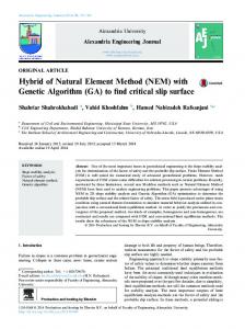
The random keys for these offspring can be sorted and the resulting bay assignments and ordering within the bays readily determined. The chromosomes of the offspring will always maintain encoding integrity for permutations. The problem of infeasibility due to violation of the aspect ratio constraints is handled using the adaptive penalty approach of Coit, Smith and Tate [4]. This approach permits infeasible solutions initially but penalizes infeasibility more as the search continues. The penalty imposed on infeasible layouts is a function of both the number of generations and the relative fitness of the best feasible and infeasible solutions yet found. This permits a broad range of search paths initially but drives the RKGA to find feasible solutions at the conclusion of the search process. The proposed random keys encoding has been compared with the encoding of Tate and Smith [15] for problems with deterministic flows and found to perform better on average. III. OPTIMIZATION APPROACH The basic objective is the minimization of a statistical bound of total material handling costs (see Figure 2 for example of an upper bound) subject to constraints on departmental shapes given a fixed total rectangular area A with fixed H and W, and fixed departmental areas, aj. There are p independent products each with an expected demand or production volume and a standard deviation per unit of time (e.g., day, week or month). Invoking the central limit theorem of sums, the probability distribution of the total material handling costs is Gaussian, even when only a few products are involved. α can be in the optimistic range (α > 0.50), or at the
expected value (α = 0.50) or in the pessimistic range (α > 0.50). To clarify this, a layout which is optimized for a small α value will have a low cost even if the quantity actually produced of products is on the high side of the forecast (where there is variability in the forecast). A layout for a large α value would perform the best when production was on the low side of the expected value of the forecast. A user would probably select a layout which performed well for production both in excess and less than the expected value of the forecast.
f( C )
C 1-α
α
M a te ria l T r a n s p o rt C o s ts (C )
Figure 2. The Objective Function can be an Upper Bound on Material Handling Costs. For each product, it must also be known which departments will be included in the product manufacture, assembly or handling. For example product 1 could be routed through departments a, c, d and g while product 2 is routed through departments c, d, e, f and g. With this formulation, the variability of the forecasts of each product can be considered separately. An established product might have low variability of forecast while a new or future product may have high variability. The product volumes, variability and routings along with unit material handling costs and departmental areas and constraints are the required information prior to the design phase. This formulation using products and their individual characteristics is very natural for managers and engineers, and averts specifying probabilities or random variable distributions. Although they are not included here, fixed costs of locating a department or of transport could also be included. Mathematically the problem formulation, using a rectilinear distance metric, is: n n p min ∑vi∑∑δijk cxj−cxk + cyj−cyk j =1 k =1 i =1 (2) j ≠k
(
)
n n ∑ σ vi∑∑δijk j =1 k =1 i =1 j ≠k p
+ z1−α
r ≤R
s.t.
j
j
2
(
− + − cxj cxk cyj cyk
∀j
where
r maximum aspect ratio of dept j R maximum allowable aspect ratio of dept j j
j
v
i
expected volume for product i per unit time where i = {1, 2, ... , p}
)
σ
2
δ
ijk
c
variance of volume of product i per unit time
vi
xj
1 if product i is transported from dept j to dept k = 0 if product i is not transported from dept j to dept k
x coordinate of dept j centroid
c
yj
z
1−α
y coordinate of dept j centroid
standard Gaussian z value for level 1- α
Since this formulation is unique, four test problems were developed using from 2 to 16 products and the 20 department areas of the Armour and Buffa problem [1]. A significant amount of routing overlap between products was included and the product mix was a diverse set of expected values and coefficients of variance (σ/µ) for each test problem. A full factorial design of experiments was conducted using the four problems to test the performance of the methodology considering alterations in the following parameters: population size (10, 25, 50), mutation rate (0.25, 0.50), random number seed (5 seeds), maximum aspect ratio (3, 5, 10), and risk level (z1-α = 0, 1, 2, 3). The first two items are GA specific parameters, the third tests pure stochastic sensitivity and the last two change the problem being solved. The maximum aspect ratio varies from very constrained (3) to hardly constrained (10) and the uncertainty ranges from expected value (0) to very optimistic (3). This full factorial experiment totaled 1440 design procedures. IV. RESULTS The results have demonstrated the effectiveness of the RKGA optimization. Its performance is relatively insensitive to parameter settings, random number seed and problem instance. More importantly, the research shows the effect of explicit consideration of uncertainty. Figure 3 shows the layout for the most constrained (maximum aspect ratio = 3) version of the 16 product problem when an implicit assumption of certainty is made (z1-α = 0) as opposed to the layout when an explicit consideration of uncertainty (z1-α = 1, 2, or 3) is made. Table 1 shows the results of when each z1-α value is used in the objective function. It can be seen that as z1-α changes, the relative contribution of the expected value and the standard deviation of total material handling costs changes. For an expected value (z1-α = 0) objective function, variance is ignored and the standard deviation of costs is large. Furthermore, where the objective function does not properly reflect the uncertainty (i.e., where z1-α of the objective function differs from that of the actual uncertainty), the designs are uniformly sub-optimal. Figure 4 shows the dominance of each of the four plant layouts as uncertainty (α) changes from expected to the optimistic side of the forecast. It can easily be seen that the design resulting from traditional methods (implicitly assumed certainty) is clearly sub-optimal when
z1-α = 0 20
13
1
19
7
9
8
2
5
4
3 12
z1-α = 2 10 1 11
3
18 6
15
17
16
14
7
14
4
12
6
2
17
8
5
6
16
20 19
13
18
1
8 7
18
15 11
17
15 10 6
2
13
2
9 7 8
5
4
3 20
16
1
9 19
19 11
4
20 13
z1-α = 3
14 5
10
11
9
z1-α = 1 3
15
16 12
10
17
12
18 14
Figure 3. Even Highly Constrained Optimal Plant Layout Design is Dependent on Uncertainty Level. Table 1. Components of Objective Function of Optimal Solutions as z1-αα Changes. Equation Equation Equation 5 Mean Standard Equation Risk Attitude 5 Value 5 Value Value for Costs Deviation 5 Value (z1-α) of Costs for z1-α=1 for z1-α=2 z1-α=3 for z1-α=0 0 (risk neutral) 14703 9733 14703 24436 34169 43901 1 (mildly risk averse) 15809 6327 15809 22136 28463 34791 2 (risk averse) 17176 5191 17176 22367 27557 32748 3 (acutely risk averse) 18788 4476 18788 23263 27739 32215 almost any degree of uncertainty is considered. This type of graph is extremely useful for an analyst to quickly ascertain the cost/uncertainty trade-offs of any particular layout design problem. Robust layouts which perform well over a variety of production scenarios can be identified. Recall that these results are for the most constrained problem as constraint lessens, even greater disparity in optimal plant designs will be observed over the studied uncertainty levels. For the less constrained versions of the problem (aspect ratio = 5 or 10), the results were similar. Table 2 shows the optimal solution of the median of five GA runs for each aspect ratio and each value of z1-α. Two trends can be easily observed. First, as the maximum allowable aspect ratio is relaxed, the material handling costs become smaller since departments can assume a longer, narrower shape which reduces centroid to centroid distance. Second, as z1-α increases, the mean costs increase while the standard deviations of costs decrease. This is the effect of optimizing an upper bound rather than simply a mean value. Only the layouts for aspect ratio = 3 and z1-α = 2 or 3 depart from this trend, where the solution identified for z1-α = 3 actually
dominates that of the solutions for z1-α = 2. Note that the values in Table 2 are somewhat different from those in Table 1. This is because the solutions in Table 2 were the result of increased length runs. V. CONCLUDING REMARKS Facility layout design is a problem that when solved properly improves the efficiency, responsiveness and profitability of an organization. Conversely, if the layout is poor, operations suffer daily until the layout is corrected, a step which is costly and time consuming. In most previous approaches, uncertainty in forecasts over the life of the layout design (which can be long) is not considered. The approach described in this paper enables the identification of physically reasonable block layouts which properly and explicitly reflect both product forecast variability and user attitude towards production uncertainty. The identification of robust layouts can be easily made through graphs such as Figure 4.
45000 z=0 z=1
40000 objective function value
z=2 z=3
35000 30000 25000 20000
crossover points
15000 10000 0.5
0.4
0.3
α v alu e
0.2
0.1
0
Figure 4. Cost Performance of Optimal Designs as Optimistic Uncertainty Increases. Table 2. Components of Objective Function as z1-αα and Aspect Ratio Change. Aspect Ratio = 3 Aspect Ratio = 5 Aspect Ratio = 10 Mean Costs Standard Mean Costs Standard Mean Costs Standard Uncertainty Level Deviation Deviation Deviation (z1-α) 0 (expected value) 13983 8741 12667 7176 10164 7631 1 (mildly optimistic) 14532 5814 14099 5474 10800 5778 2 (fairly optimistic) 15970 4562 15350 4513 12607 4681 3 (very optimistic) 15832 4562 15629 4415 14831 3778 References [1] Armour, G.C. and E.S. Buffa, “A heuristic algorithm and simulation approach to relative allocation of facilities.” Management Science, 1963 9, 294-309. [2] Bean, J.C., “Genetics and random keys for sequencing and optimization,” ORSA Journal on Computing, 1994 6, 154-160. [3] Cheng, R., M. Gen, and T. Tozawa, “Genetic search for facility layout design under interflows uncertainty.” Japanese Journal of Fuzzy Theory and Systems, 1996, to appear. [4] Coit, D.W., A.E. Smith, and D.M. Tate, “Adaptive penalty methods for genetic optimization of constrained combinatorial problems.” INFORMS Journal on Computing, 1996 8, 173-182. [5] Garey, M.R. and D.S. Johnson, Computers and Intractability: A Guide to the Theory of NP-Completeness. 1979, New York: W. H. Freeman and Company. [6] Kouvelis, P., A.A. Kurawarwala, and G.J. Gutierrez, “Algorithms for robust single and multiple period layout planning for manufacturing systems.” European Journal of Operational Research, 1992 63, 287-303. [7] Norman, B.A. and J.C. Bean, “Operation scheduling for parallel machine tools,” Department of Industrial Engineering, University of Pittsburgh Technical Report 95-9, 1995, under revision for IIE Transactions. [8] Norman, B.A. and J.C. Bean, “A random keys genetic algorithm for job shop scheduling,” Department of Industrial Engineering, University of Pittsburgh Technical Report 96-5, 1996, accepted for publication in Engineering Design and Automation. [9] Norman, B.A. and J.C. Bean, “A genetic algorithm methodology for complex scheduling problems,” Department of Industrial Engineering, University of Pittsburgh Technical Report 96-7, 1996, under review at Naval Research Logistics Quarterly. [10] Rosenblatt, M.J. and D.H. Kropp, “The single period stochastic plant layout problem.” IIE Transactions, 1992 24, 169-176. [11] Rosenblatt, M.J. and H.L. Lee, “A robustness approach to facilities design.” International Journal of Production Research, 1987 25, 479486. [12] Shore, R.H. and J.A. Tompkins, “Flexible facilities design.” AIIE Transactions, 1990 12, 200-205.
[13] Tam, K.Y., “Genetic algorithms, function optimization, and facility layout design.” European Journal of Operational Research, 1992 63, 322-346. [14] Tam, K.Y., “A simulated annealing algorithm for allocating space to manufacturing cells.” International Journal of Production Research, 1992 30, 63-87. [15] Tate, D.M. and A.E. Smith, “Unequal-area facility layout by genetic search.” IIE Transactions, 1995 27, 465-472.