Randomization tests in language typology 1
Dirk P. Janssen , Balthasar Bickel2 and Fernando Zúñiga
3
1
Psychology Department, University of Kent, Canterbury, UK Linguistics Department, University of Leipzig, Leipzig, Germany 3 Centro de Estudios Públicos, Santiago, Chile 2
[ version 21; 08 September 2005 ]
Abstract
Two of the major assumptions that statistical tests make (random sampling, distribution of the data) are not tenable for most typological data. We suggest to use randomization tests, which avoid these assumptions. Randomization is applicable to frequency data, rank data, scalar measurements and ratings, so most typological data can be analyzed with the same tools. We provided a free computer program, which also includes routines that help determine the degree to which a statistical conclusion is reliable or dependent on a few languages in the sample. Keywords statistics; randomization; fisher exact test; chi-square test; interval data
Address for Correspondence: Balthasar Bickel, Institut fuer Linguistik, Beethovenstrasse 15, D-04107, Leipzig, Germany Email:
[email protected],
[email protected],
[email protected]
Randomization tests
-1-
1.1. Random sampling Most statistical tests make a number of assumptions which are not always tenable for typological data. The two most important assumptions concern random sampling and the distribution of the data. We will discuss these two points in turn. The assumption of random sampling means that the cases under study (the sample) are randomly drawn from the cases that we want to make a statement about (the population). Random sampling is ideally done with a random number generator, which generates a number between 1 and the number of languages we have available. This way, the sample is constructed in a truly random fashion. The requirement of random sampling has also been called ‘independence of selection of cases’, because in a truly random sampling procedure, whether we sample language A does not influence the chance of sampling language B. The term ‘random sampling’ is preferable, because it makes it clear that sampling does not require ‘independence of cases’ in the sense that each and every case in the sample is independent of all the others. Independence of cases cannot be a requirement of any type of sampling, as the languages in the sample could never be representative of the population under such a restriction. In a truly random sample of African languages, it is very likely to encounter a number of Bantu languages. This is correct because the chance of having sampled Zulu should not influence the chance of sampling Luganda. Of course, these two languages are not independent cases for comparative purposes, but that does not matter for sampling procedures. Random sampling implies that all cases in the population must have the same chance of being included in the sample. A statistical test can therefore never make a statistical conclusion about ‘all possible human languages’ or ‘all human languages that ever existed’, as only a very tiny fraction of languages actually has a chance of
Randomization tests
-2-
being sampled at all: those spoken now or known from written records. Random sampling is the hallmark of statistics, because it makes it very unlikely that there is any systematic bias in the sample. But what about accidental biases: What if in a randomly drawn sample of language of Europe, Basque happens to be not included? Does this restrict our population to ‘The languages of Europe, excluding Basque’? Or, if in a randomly drawn sample of Europe, we happen to end up with five Germanic and only one Romance language, does this change the population? Luckily, it does not — if all languages, including Basque, all Romance and all Germanic languages, had the same a priori chance of being included in the sample. In that case, the conclusions are still valid for the languages in Europe. 1.2. Strata Such a conclusion might be statistically valid, but many typologists will be unhappy with it. In typology one generally wants to be able to tell genealogical factors apart from structural or areal factors (at least as far as the genealogy is known from historical linguistics). So, if a sample of European languages lacks Basque, or if contains many more Germanic than Romance languages, any distributional pattern that we find is likely to be influenced as much by genealogical relatedness (IndoEuropean, Germanic) as by the typological (structural, areal) factors of interest. In this situation, it is impossible to determine the relative contribution of each factor. Genealogical relatedness is what is called a confounding factor and the standard statistical solution for this is stratification: We randomly sample languages but ensure that the same number of languages is taken from each stratum. This is very similar to the way in which opinion polls ensure that the same number of men and women are included in order to avoid any gender bias in sampling. The statistical conclusion based on a stratified sample of languages has the same population as a conclusion based on a random sample: all European languages. The
Randomization tests
-3-
only difference is whether the researcher thinks that the influence of the strata (genera) should be controlled for. Stratification is common statistical practice; it works well for large and welldescribed families. When it comes to smaller families, however, stratification may lead to samples that are no longer random within the stratum: many genera are so small (or only a small number of their languages is sufficiently documented) that a random choice cannot be made. In the case of isolates like Basque, only one language can be chosen. 1.3. The level of sampling It has independently been argued (Dryer 1989, 2000) that the correct level of analysis in quantitative typology is not the level of the language, but that of the genus. If the genus is the correct level of sampling, genera should be sampled at random and the population would be 'all genera’ (in the world, in area X, etc.). This way, the problem of random selection within very small strata is avoided. Each genus is one data point in the sample. In most cases, the typological features of this data point will be represented simply by the single language of the genus that is at all described. If more than one language from a genus is known, the data point can be inferred from what is judged to be representative of the genus, or simply from what is the best described language, or from a random choice of the described languages of the genus. The latter solution would be more popular among statisticians, as it avoids any researcher bias in selecting the 'most representative' language, but the other solutions are far more reasonable in typology because they allow one to better control for genealogical information and to favor better descriptions. An alternative, which results in a richer sample, is to add more than one language per genus. But since each genus would have to be represented by the same number
Randomization tests
-4-
of languages, and many genera include only one (isolates), or only one sufficiently described language, this alternative is impractical for most purposes. 1.4. Complete sampling When sampling genera, or similar genealogical units, one will want to include as many genera as possible, so as to make the sample ever more representative. The most representative sample will include a data point for each genus in the area of interest (e.g. the languages of Eurasia, of Africa, etc). In statistical terms, taking all genera amounts to a complete sample. What happens to our statistical test in this case? The surprising answer is that classical statistical tests are not valid for complete samples. A statistical test is a means to draw conclusions about the population from properties of the sample. More concrete, a statistical test answers the question whether a difference observed between the sample groups is likely to hold for the population groups. If the sample groups and the population groups are identical, classical statistical tests simply do not apply and any statistical result will be mathematically meaningless. 1.5. Possible solutions However, in many cases in language typology, it is both possible and desirable to create complete, or near-complete, samples of genera. This is especially true in smaller-scale areal typology where the number of genera is small. How can we proceed? Drawing random subsamples for statistical purposes would be one solution. But chosing, say, 10 out of 15 genera in an area would mean throwing out valuable information. What other options are there? One option is to deny the use of statistical testing altogether or take the perspective that because the populations are sampled completely, statistical testing is not necessary. There are two problems with this position. First, if in one region 8 out of 10 genera prefer the verb to occur in sentence final position and in the other Randomization tests
-5-
region 7 out of 10 genera prefer this, who can decide whether this a meaningful difference (cf. Cysouw, in press)? Secondly, this approach disregards the arbitrariness of selecting languages from each genus: If other languages were taken, would the difference in word order still be the same or would it disappear? A better solution is to use a different type of statistical test, one that does not try to make predictions about the population but speaks only of the cases included in the sample. There are a number of statistical test that have this property, like the chisquare test. These tests are often called non-parametric tests, because they do not aim to estimate population parameters. We will advocate the use of randomization tests here, which are not only non-parametric but also distribution-free. 2.1. The distribution of the data The second major assumption that statistical tests make is that of a certain distribution of the data. For tests like the t-test or the Anova, these requirements are quite strict and researchers are trained to always first establish the validity of the test by testing the distribution requirements. For other tests, the requirements on the distribution are less well-described. The commonly used chi-square test (officially known as the Pearson chi-square test) is a non-parametric test that considers the numbers in a table of counts. For each cell, the actual number that was observed is compared to a prediction based on the row and column totals, i.e. on what one would expect if the row and column labels had no influence on the cells. A summation over all cells results in the Pearson chi-square quantity (see Formula 1).
Randomization tests
-6-
[formula 1] The Pearson chi-square quantity
2.2. The chi square test How can we decide whether the observed counts are significantly different from the expected counts? Pearson observed that, for large enough numbers, the distribution of the Pearson chi-square quantity is quite similar to that of the independently known χ2 distribution. (To avoid confusion, we will use chi-square for the quantity and the symbol χ2 for the distribution). Only with help of the χ2 distribution can a Pearson chi-square quantity be mapped to a probability level (e.g., p = 0.12) and a significance value (e.g., not significant).1 This means that the Pearson chi-square is non-parametric, because it does not extrapolate from a sample to a population, but it is not distribution-free, because the χ2 distribution is needed to compute p-values. The estimate based on the χ2 distribution is perfect as long as the numbers in the cells are large enough. Regrettably, there is no strict definition of 'large enough'. The rule of thumb that is usually given is that no cell should have an expected count smaller than five (Howitt & Cramer, 2005). An alternative version of this rule states that at least 80 percent of the expected numbers must be larger than five and all should be at least one (Cochran, 1954). Finally, how close the χ2 distribution and the Pearson chi square quantity are also depends on the total number of data points and on their distribution over the table. These are all highly problematic restrictions in typology, because empty cells and cells with small values are particularly interesting. They suggest heavy biases in the data.
Randomization tests
-7-
2.3. Fisher exact test For the specific case of a 2-by-2 table of counts, a non-parametric and distributionfree test has been proposed by R.A. Fisher in the 1930s. The Fisher Exact test can be run in all major statistics packages and in various other tools, and is preferable to the Pearson chi-square in all cases of 2-by-2 tables. Similar to the randomization tests we will advocate below, the Fisher Exact considers all possible ways in which a 2-by-2 table can be constructed without changing the margin totals. In a standard typological table used for an areal comparison of a certain feature, the margins totals are the number of languages in the two regions and the total number of languages that have or do not have the feature under study, see Table 1.
[Table 1] Example 2-by-2 table: Number of languages which have Multiple Possessive Classes (Bickel & Nichols 2003, Nichols & Bickel 2005)2 Multiple Possessive Classes (Observed) No Yes Total 10 4 14
Expected Area No Yes Total A: Caucasian and 12.8 30.2 14 Himalayan Enclaves B: Rest of Eurasia 33 0 33 1.2 2.8 33 Total 43 4 47 43 4 47 Fisher Exact Test: Columns are not independent of rows, p=0.00561 (two-sided) Chi-square Test: Invalid test due to two expected values lower than five, p=0.00832 (two sided) Randomized Chi-square Test (see 3.1 below): Columns are not independent of rows, p=0.0054 (two-sided)
The number of languages taken from each area is pre-determined by the researcher. The total number of languages with the feature ‘has multiple possessive classes’ is the result of research. The total number of languages without the feature is fixed, as the total number of languages is known from summing areas A and B. Taken together, the assumption of fixed margin totals seems typologically justified. As said, the Fisher Exact test will consider all possible other 2-by-2 tables with the same margin totals as the observed table. There are usually several hundreds or
Randomization tests
-8-
several thousand such tables, depending on the number of data points. The more exceptional the observed table is compared to the range of other possible tables, the less likely it is that the observed table occurred by chance. If, on the other hand, the observed table is very similar to a large number of other possible tables, it is likely that it is chance and not some areal distribution that caused the observed table. We will return to the issue of chance given a range of possibilities below, but first we will consider what happens if we are not interested in counts alone.3 2.4. Nominal, rank and interval data The typology shown in Table 1 assigns one of two labels to each language (the language has or does not have multiple possessive classes). Other typologies distinguish three or more labels. For example, Östen Dahl's typology of the words for 'tea' has ‘derived from cha’; ‘derived from te’; and ‘other’ (Dahl 2005). In these cases, a statistical analysis can best consider the frequency with which each label occurs. For other typologies the labels can be ordered in some way, leading to a rank measurement. Consider Ian Maddieson’s consonant inventories entry (Maddieson, 2005) in the World Atlas of Language Structures (WALS), which uses the labels small; moderately small; average; moderately large; and large. Running frequency statistics on rank measurements is not incorrect, but such an analysis is insensitive to the fact that moderately large and large are much closer to each other than small and large are. It is important for rank-based analyses that all labels can be ordered. If there is an 'other' label that cannot be compared to the others because it is a mixed bag of cases, we can either only use frequency statistics, or we have to exclude all languages of the 'other' type. In WALS, David Gil's typology of 'Genitives, adjectives and relative clauses' (Gill, 2005) shows another type of incomplete ranking (see Table 2). It is probably
Randomization tests
-9-
impossible to objectively rank labels 2 to 5. To use rank-statistics for these data, one would create a three-way distinction between weakly, moderately and highly differentiated. Of course, this would mean loss of precision in the data, as we no longer distinguish between different types of moderately differentiated languages. An ideal analysis would therefore consider both a frequency based analysis of all data and a rank-based analysis of the collapsed data.
[Table 2] David Gil's typology of Genitives, adjectives and relative clauses, from Gil (2005) Original label 1. weakly differentiated 2. genitives and adjectives collapsed 3. genitive and relative clauses collapsed 4. adjectives and relative clauses collapsed 5. moderately differentiated in other ways 6. highly differentiated
Ranked label 1. weak 2. moderate 2. moderate 2. moderate 2. moderate 3. strong
Rank data can be analyzed with classical non-parametric tests like the MannWhitney U-test (for 2 groups) or the Kruskal-Wallis test (for more than 2 groups). These tests are supplied in statistical packages and are described in textbooks like Howitt and Cramer (2005). Finally, there are interval measurements (including so-called ratio measurements, which can be treated as interval measurements for all statistical purposes). The crucial difference between a rank and an interval measurement is that, for interval measurements, the distance between all values is the same. There are currently only few typological interval measurements, but there are a number of typologies that come close enough to be analyzed as interval measurements. An example is Bickel & Nichols’ (2005) typology of verbal inflectional synthesis. However, one can also use interval statistics on typologies that use a rating scale to express how much each languages exhibits a feature, if the rating scale has at least 5 (preferably 7) levels.
Randomization tests
-10-
Maddieson's (2005) consonant classification into 5 ranks could therefore also be analyzed as interval data, which brings several benefits in terms of data analysis.
3.1. Randomization tests Considering the variety of measurement types that typologists can encounter and the problems with sampling and distribution that were mentioned above, we suggest using randomization tests (also called Monte-Carlo tests or permutation tests) throughout in typology. These tests are non-parametric and distribution-free, and they can handle frequency, rank and interval data in similar ways. The statistical question that underlies all randomization testing is whether the obtained data could have been generated by chance. Consider the frequency tables in Table 3, of which the first is the observed table and the others are two of the alternative tables with the same margin totals. We assume that, if chance has it, the values of the feature (F1 to F3, these could be the three labels for 'tea' or any other classification) are randomly distributed and each area therefore has about the same number of languages with each label. The alternative table 2 shows what a chance distribution of the feature labels might look like. Clearly, the observed distribution is unlike a chance distribution, as F1 is relatively common in Area A, F2 in Area B and F3 in Area C. The Pearson chi-square quantity is a sum of the differences between expected and observed values. The expected values are derived from the margin totals under the assumption that there is no systematic pattern in the data. This means that we can measure how far removed a table is from a pure chance distribution by looking at its Pearson chi-square quantity. For the three tables in Table 3, the chi-square quantities are 10.6, 2.9 and 1, which corresponds with the idea that the observed table is furthest removed from chance.
Randomization tests
-11-
In a classical Pearson chi-square test, we determine the probability of the chisquare value of 10.6 (for the observed table) from the χ2 distribution. A randomization test will instead look at about 10,000 alternative tables with the same margin totals. For each of these tables, a Pearson chi-square quantity is computed. If the observed chi-square value is much higher than most of the values that are found in the alternative tables, the observed table is unlikely to be due to chance. In the example in Table 3, the observed value of 10.6 is indeed higher than the two alternative values (2.9 and 1) and compared to another 9998 tables, it will turn out to be significantly higher.4
[Table 3] Example of randomization testing: Observed data and two alternatives that will be considered by a randomization test
Observed Table Feature value F1 F2 F3 Area A 2 0 1 Area B 0 2 0 Area C 1 0 3 3 2 4
3 2 4 9
Alternative Table 1 Feature Value F1 F2 F3 Area A 1 1 1 Area B 0 1 1 Area C 2 0 2 3 2 4
3 2 4 9
Alternative Table 2 Feature Value F1 F2 F3 Area A 1 1 1 Area B 1 0 1 Area C 1 1 2 3 2 4
3 2 4 9
3.2. Comparing classical and randomized chi square A standard test for the observed table returns a Pearson chi-square value of 10.6 which (using the χ2 distribution with 4 degrees of freedom) has p = 0.03195. The statistical software warns us that the result cannot be trusted, as the rule-of-thumb criterion for a classical Pearson chi-square test are violated (many cells with expected value under five). A randomized test based on 10,000 replications results
Randomization tests
-12-
in p = 0.0209, more than a full percent point less, and this test is valid. Even though the difference between the p-values in this example is not very large, there are a number of advantages of the randomized chi-square test over the classical one: First, the classical test is not applicable because its assumptions (expected values all five or larger) are violated. Second, the classical test gives a conservative estimate which results in too few tables being significant. Third, the randomized chi-square test does not make any assumptions about the population or the distribution of the data, which makes it universally applicable. The randomized test also has drawbacks. These tests are, for example, not yet as widely used as classical tests. Statisticians use randomization (and its relative, bootstrapping) routinely, but, with the notable exception of genetics and a few other sciences, other fields have not caught up yet. Furthermore, not all statistical software packages support these tests. Again, this is changing rapidly (SPSS now provides a related module for the Windows platform), and we have created some easy-to-use scripts for the free statistical software called 'R'. It used to be the case that computing statistics on 10,000 random tables required a lot of computer power and a lot of patience. With modern computers, this is no longer an issue. Our scripts used less than a second to compute the randomized chi-square values mentioned above. Finally, because the significance is the result of a simulation, a slightly different result will be obtained if the same test was run again. With 10,000 replications, the significance level will be precise at the 0.001 level and any further variation is harmless. Further discussion of the benefits and drawbacks of randomization tests can be found in Edgington (1995), Manly (1991) and Sprent (1998).
Randomization tests
-13-
3.3. Randomized Anova We will now briefly consider how the randomization method can be used for interval data. Table 4 shows the distribution of inflectional verbal synthesis over two areas, the Causasian and Himalayan enclaves versus the rest of Eurasia (Bickel and Nichols, 2003, 2005). Two things are obvious from looking at these data: The Enclaves seem to have overall higher values for synthesis than the Rest of Eurasia, but the counts for the Enclaves are very small. [Table 4] Inflectional Synthesis of the Verb, data for Caucasian and Himalayan Enclaves (Enclaves) versus the rest of Eurasia (R.Eurasia) (from Bickel & Nichols 2003, 2005)
Enclaves R.Eurasia Total
Observed 0 2 0 0 1 1 1 1
values of synthesis 3 4 5 6 0 0 3 3 1 3 3 9 1 3 6 12
7 1 5 6
Enclaves R.Eurasia Total
Expected 0 2 0.3 0.3 0.7 0.7 1 1
values of 3 4 0.3 1 0.7 2 1 3
derived from column 7 8 9 10 2.1 0.7 0.7 1.7 3.9 1.3 1.3 3.3 6 2 2 5
synthesis, 5 6 2.1 4.1 3.9 7.9 6 12
8 1 1 2
9 0 2 2
10 1 4 5
11 0 2 2 and 11 0.7 1.3 2
12 5 0 5
13 0 2 2
14 0 1 1
row totals 12 13 14 1.7 0.7 0.3 3.3 1.3 0.7 5 2 1
15 1 0 1
18 1 0 1
20 1 0 1
22 1 1 2
25 1 0 1
15 0.3 0.7 1
18 0.3 0.7 1
20 0.3 0.7 1
22 0.7 1.3 2
25 0.3 0.7 1
Descriptive statistics Enclaves: 19 cases, mean 11.5, median 12, standard deviation 6.1 R.Eurasia: 36 cases, mean 7.5, median 6.5, standard deviation 4.0 Total: 55 cases, mean 8.9, median 7, standard deviation 5.1
A classical Anova (analysis of variance) would be a good test for these data, as it can tell us whether there is a difference between the values of synthesis in each region and, if so, which regions differ from each other. However, the data are not even close to normally distributed and certainly not randomly sampled, which would make any application of a classical Anova flawed. Because this is a complete sample of the Enclaves, the results of this test would be, as argued in Section 1.4, mathematically meaningless. Still, if we compare the observed counts with the expected counts, it is clear that Randomization tests
-14-
the number of enclave languages with a synthesis value of 12 is much higher than is expected (5 observed, 1.7 expected). Also, both mean and median synthesis value for the Enclaves are much higher than for the Rest of Eurasia, which is partly due to the fact that the Rest of Eurasia has consistently fewer languages at the high end of the synthesis scale (0 observed, 0.7 expected) and more languages at the lower end of the scale (1 observed, 0.7 expected). This observation can be made more statistically precise using a randomization method. A randomized Anova works like the randomized chi-square test described above. For each alternative table, languages are assigned to cells of the table at random, with the constraint that the margin totals stay the same. For each table, an Anova Fvalue is computed. The F-value expresses how large the differences between the groups are, relative to the differences within the groups. The assumption is that the F-value for each alternative table might not be fully accurate because of the low numbers in the Enclaves, but the ordering of F-values is correct. If the observed F-value is much higher than what is routinely found among random alternative tables, the observed table is significant because it is unlikely to be due to chance. For the comparison between the Enclaves and the rest of Eurasia, the randomized Anova with 10,000 alternatives yields p=0.0054, which is significant and (in this case) only marginally different from the result of the classical Anova: Thus, we can safely conclude that languages in the Enclaves tend to have higher synthesis degrees than those in the rest of Eurasia. 4.1. Reliability and misclassification After any successful statistical analysis has been done, one may wonder what would have happened if a problematic language had been classified or analyzed differently. Additionally, what would have happened if we had chosen other languages from each
Randomization tests
-15-
genus? To some extent, this is an empirical problem that cannot be solved by any statistical procedure. However, what statistics can do is estimate the degree to which our data is sensitive to the issue of misclassification and thereby help us determine how reliable our findings are. We propose a method for this, which involves computing the statistics on all alternative scenarios that are one or more misclassifications away from our observed data and graphing the results. If there are many ways in which one misclassified languages changes the significance of the results, we have to be careful when interpreting the data. If one or a few misclassified languages do not make any difference, we can be more certain of our case. The reliability graph is closely related to randomization testing. Recall that randomization testing is based on finding alternative tables with the same margin totals. If, instead, we alter the margin totals in such a way that only the total number of languages (the sample size) stays the same, we can explore the issue of misclassification. As an example, we examine the data on possessive classes (POSSCL) from Table 1. The two categories are again languages with or without possessive classes. For the 2-by-2 count table created by looking at this dichotomization for the Enclaves versus the Rest of Eurasia, a reliability landscape is produced as shown in Figure 1.
Randomization tests
-16-
8 7 6 5 4 3 2 1
9
8
7
6
5
4
3
2
1
0
0
Positive cases for Group2 (Area=R.Eurasia)
9
Positive cases for Group1 (Area=Enclaves)
[Figure 1] Reliability Landscape for a 2-by-2 table, with increasing levels of cross-hatching indicating significance at or below 0.10, 0.05 and 0.01 levels. White squares are not significant, p>0.10.
The bold-faced square on the bottom row of the figure symbolizes the observed data point. This point has coordinates (4,0), that is, there are 4 POSSCL languages in the Enclaves (plotted from left to right) and zero in the rest of Eurasia (plotted updown). The shading of this square signals a significance level of p


![[PDF] Randomization Tests, Fourth Edition - Google Sites](https://m.moam.info/img/260x300/pdf-randomization-tests-fourth-edition-google-site_64780f3b097c474b228cc55a.jpg)