Rank Based Binary Particle Swarm Optimisation for Feature Selection in Classification Majdi Mafarja
Nasser R. Sabar
Department of Computer Science, Birzeit University Birzeit
[email protected]
Department of Computer Science and Information Technology, La Trobe University Melbourne, Australia
[email protected]
ABSTRACT Feature selection (FS) is an important and challenging task in machine learning. FS can be defined as the process of finding the best informative subset of features in order to avoid the curse of dimensionality and maximise the classification accuracy. In this work, we propose a FS algorithm based on binary particle swarm optimisation (PSO) and k-NN classifier. PSO is a well-known swarm intelligent algorithm that have shown to be very effective in dealing with various difficult problems. Nevertheless, the performance of PSO is highly effected by the inertia weight parameter which controls the balance between exploration and exploitation. To address this issue, we use an adaptive mechanism to adaptively change the value of the inertia weight parameter based on the search status. The proposed PSO has been tested on 12 well-known datasets from UCI repository. The results show that the proposed PSO outperformed the other methods in terms of the number of features and classification accuracy.
CCS CONCEPTS • Computing methodologies → Feature selection;
KEYWORDS Feature Selection, Classification, Particle Swarm Optimisation ACM Reference Format: Majdi Mafarja and Nasser R. Sabar. 2018. Rank Based Binary Particle Swarm Optimisation for Feature Selection in Classification. In Proceedings of The International Conference on Future Networks and Distributed Systems (ICFNDS 2018). ACM, New York, NY, USA, Article 4, 6 pages. https://doi.org/10.475/ 123_4
1
INTRODUCTION
Machine learning techniques have been widely used in various fields, e.g., image classification, pattern recognition, and disease classification [4]. Many fields involve huge datasets due to the advanced data collection tools and technologies. These fields suffer from the curse of dimensionality [14] and thus data reduction becomes a mandatory step to process them in a moderate amount of time. Feature Selection (FS) is a primary dimensionality reduction Permission to make digital or hard copies of part or all of this work for personal or classroom use is granted without fee provided that copies are not made or distributed for profit or commercial advantage and that copies bear this notice and the full citation on the first page. Copyrights for third-party components of this work must be honored. For all other uses, contact the owner/author(s). ICFNDS 2018, June 2018, Amman, Jordan © 2018 Copyright held by the owner/author(s). ACM ISBN 123-4567-24-567/08/06. . . $15.00 https://doi.org/10.475/123_4
form that aims to select the most informative subset of features from the original dataset (or set) to reduce the dimensionality of data. Over the years several FS tools have been proposed. A traditional FS tool consists of two components: evaluation criterion and selection (search) algorithm. The evaluation criterion is used to assess the quality of the selected subset of features. It can be either filter, wrapper or embedded [29]. Filter approaches are simple and require light computational time since they depend on the relations between data itself when evaluating the selected subset, without employing an external evaluator [27]. Wrapper approaches are considered more efficient than filters but they may suffer from high computational cost. The main role of the selection (search) algorithm is select the most infomrative subset of features from the given set. Various search strategies have been used as a selection (search) algorithm [13]. They can be categorised into: complete, random, and heuristic search. In complete search, all possible feature subsets should be generated and evaluated to select the best feature subset. With the curse of dimensionality, this approach becomes impractical option. Random search selects feature subsets randomly. This approach may find a subset faster than the complete search, but at the worst case, it may perform worst than the complete search without finding the best subset. Heuristic search or meta-heuristics algorithms have been widely used in FS as they are very efficient, easy to implement and can handle large scale data. A branch of meta-heuristics algorithms is the Swarm Intelligence (SI). SI algorithms mimic the natural behaviour of some creatures that live in folks or groups like folks of birds and ants [10]. Various SI algorithms have been utilised to tackle the FS problem in the literature such as GA [8], PSO [30], Ant Colony Optimization (ACO) [9], DE [31], Artificial Bee Colony (ABC) [32], Grasshopper Optimisation Algorithm (GOA) [20] and Particle Swarm Optimisation (PSO) [3], [28]. For more FS approaches, readers can refer to [1, 6, 15–19, 21, 24]. The PSO [5] is a primary SI algorithm that inspired from the self-organisation behaviour of birds. PSO is a population-based algorithm that maintains a swarm of particles. Each particle represents a complete solution to the problem at hand. PSO uses the so called velocity and position update equations to search for better solutions. In PSO, the optimisation process is accomplished in two phases: exploration and exploitation. In exploration, the whole feature space is searched to find new subsets in a different areas whereas in exploitation phase the already existing subsets are further improved. However, to get high quality solutions (subset of features) PSO need to adaptively alternate between these two
phases. This is because having more exploitation than exploration, the PSO will get stuck at the local optima. At the same time, the PSO will lose some best solutions if it went far in exploration. In PSO, the exploitation and exploration phases are controlled by the inertia weight parameter. That is at the early stages of the optimisation process, PSO should explore many areas in the search space to find candidate solutions of the fittest attraction basins. Then at the later stages, the exploitation occurs around the discovered solutions in the previous space. However, the key challenging is how to have a proper inertia weight parameter that can cope with various problem characteristics. Several strategies were proposed to adaptively change this parameter. Harrison et al. [7] provided a comprehensive study about the used updating strategies for the inertia weight parameter. In this work, we use an adaptive update strategy to adjust the value of the inertia weight parameter based on the search state. Instead of using static inertia values for all solutions, each solution will have a different inertia weight value based on its rank in the swarm. To assess the performance of the proposed PSO, twelve benchmark datasets were used and the result are compared with three similar approaches from the literature. The results showed the influence of having a proper control strategy on enhancing the performance of PSO algorithm. The rest of this paper is organised as follows: Section 2 presents the methodology which consists the basic PSO algorithm and the proposed FS tool. In Section 4, the experimental results are presented and analysed. Finally, in Section 5, conclusions are given.
2
j
j
j
j
j
(1)
j
j
vi (t + 1) = ω 1vi (t) +c 1r 1 (pBesti −x i (t)) +c 2r 2 (дBest j −x i (t)) (2)
2.2
Binary Particle Swarm Optimization
Binary PSO (BPSO) was proposed to deal with discrete optimisation problems. In BPSO, a solution (particle position) is represented by zeros and ones. Hence, the personal best (pBest) and global best (дBest) are restricted into "0" and "1". According to Kennedy and Eberhart [11], Mirjalili and Lewis [25], PSO can be converted into a binary version by using a transfer function that maps the velocity values to a real number between 0 and 1 as can be seen in Figure 1. In BPSO, the particle’s velocity and particle’s position are updated using Equation (3) and Equation (4). 1 1 + e −v(t ) where rand is a random number ∈ [0, 1]. ( 1 If rand < S (v(t + 1)) x(t + 1) = 0 Otherwise S (v(t)) =
(3)
(4)
where S(v(t)) is the Sigmoid function as depicted in Figure 1 1 0.9
METHODOLOGY
0.8
In this section, we first present the basic PSO algorithm, followed by the binary PSO and the the proposed FS approach.
0.7 0.6
T(V)
2.1
j
x i (t + 1) = x i (t) + vi (t + 1)
Particle Swarm Optimisation (PSO)
0.5 0.4
The PSO algorithm [5] is a population-based optimisation algorithm that operates on a swarm of particles. In PSO, each particle has two components known as the particle position and particle velocity. Particle’s position represents a solution to given optimisation problem. Each solution is represented by vector of N real numbers, where N is the size (dimensionality) of the given problem. Particle’s velocity represents the speed and direction that a particle should move in the search space. Both particle position and particle velocity are updated using Equation (1) and (2). In these equations, x represents the particle position and v is the particle velocity. pBest is the best personal position found by the i t h particle and дBest is the global best position found by the whole swarm. c 1 and c 2 are the acceleration parameters. r 1 and r 2 are two random variable in the interval [0, 1]. ω 1 is the inertia weight which controls the balance between exploration and exploitation phases. The main steps of PSO are as follows:
0.3 0.2 0.1 0 -10
-5
0
5
10
V
Figure 1: Sigmoid Transfer function
3
THE PROPOSED APPROACH
In this section, we discuss the main part of the proposed approach for FS. It consists of two parts: FS algorithm and the evaluation criterion. In the following subsections, the details of both parts will be presented.
(1) (2) (3) (4)
Initialise PSO parameters. Evaluate the fitness value of the swarm. Update the personal best (pbest) and global best (дbest). Update the velocity and position of each particle using Equation (1) and Equation (2). (5) Check the stopping condition; if satisfied stop and return the best particle (solution); otherwise go to Step 2.
3.1
FS algorithm
In this work, we use BPSO to search for the best subset of features from the given dataset. BPSO is well suited to deal with discrete problems such as FS. Similar to a traditional PSO, BPSO needs to find the proper value of the inertia weight parameter (ω). ω has 2
to ωmax will be given to the worst solution. In rank based BPSO (RBPSO), each solution is represented as a binary vector with N elements, where N is the number of features in a dataset. If a vector’s element value is 1, then the corresponding feature is selected, otherwise, not selected.
crucial impact on the performance of BPSO. In basic PSO and BPSO, ω is fixed for all particles regardless of the search performance. This indicates that particle positions will be updated without considering their fitness value, i.e., the low-quality solutions will be treated as the high-quality ones. This can lead to low quality solutions as the search performance is often miss-leaded by bad quality ones. Thus, there is a need for a proper updating strategy for ω that takes into account the fitness values of all particles. To address this issue, in this work, we use an adaptive updating strategy for ω, originally proposed in Panigrahi et al. [26]. In this strategy, all particles (solutions) will be ranked based on their fitness values. The solutions with high fitness values will have small ω values, while high values of ω will be given to the low-quality solutions. A small value of ω implies low-velocity value, i.e., more exploitation and slowly moves towards the global optimum compared to the solutions with large ω values. To achieve this, the value of ω will be adjusted using solution rank in the swarm, where the best solution will be ranked one while worst one will be ranked the last as calculated by Equation (5). ! R(i) (5) w(t) = wmin + (wmax − wmin ) N
3.2
The second important part in designing FS tools is the evaluation criterion. The evaluation criterion examines how good the selected subset of features. In this work, the evaluation criterion is implemented as a wrapper approach. When designing a wrapper FS algorithm, two perspectives should be taken into account: the performance of the learning algorithm (e.g., classification accuracy), and the number of selected features. We therefore used a fitness function that considers both criteria as in Equation (6). |n| (6) |N | where Err r at e represents the classification error rate, |n| and |N | are the number of selected features and the number of original features in the dataset respectively, α and β are the weights of the classification error rate and selection ratio, α ∈ [0, 1] and β = (1 − α) adopted from [23]. In this work, we use the k-NN classifier ( [2]) to calculate the accuracy of the selected subset of features. From the above equation, its evident that the designed fitness function balances between the classification accuracy, which is the complement of the classification error rate, and the number of selected features in the tested solution. Fitness = α · Err r at e + β
where R(i) indicates the rank of the i t h particle (solution) in the swarm (population), N represents the swarm size. ωmin and ωmax are the minimum and maximum values of ω. In Figure 2, it can be seen that the rank-based ω is oscillating during the search process, while the linear decreasing strategy gives a value to a solution regardless its fitness value. In this figure, two solutions from the rank based PSO were used in addition to a linear based PSO to show that each solution has a different ω values depending on its fitness value.
4
EXPERIMENTAL RESULTS
0.75
In this work, Matlab is used to implement the proposed approach and all experiments were executed on a PC with Intel Core i5 processor, 2.2 GHz CPU and 4 GB of RAM. A wrapper approachbased on the K-NN classifier (where K = 5 [22]) is used to generate the best reduct. In the proposed approach, each dataset is divided randomly using different seeds according to the Train/Test model; where 80% of the samples were used for training purposes, and the remaining samples for testing. The parameter settings of the proposed approach are listed in Table 1.
0.7
Table 1: The parameters settings
0.9 0.85 0.8
Inertia Weight Value
Evaluation criterion
0.65
Parameter 0.6 0.55
Population size
20
Number of iteration
200
Dimension
0.5
Number of runs for each technique
0.45 0.4 0
20
40
60
80
100
Iteration Number
Figure 2: Inertia Weight Values Over the Iterations
Number of features 30
α in fitness function
0.99
β in fitness function
0.01
wmin wmax
0.4 0.9
k
From the above equation, the best solution (ranked one), will be given a value that is very close to ωmin , while a big value close
Value
5 [23]
In this paper, twelve well-known datasets from the UCI data repository [12] were utilised to assess the efficacy of the proposed 3
Table 3: Comparison between BPSO and RBPSO in terms of classification accuracy
approaches as in Table 2. For comparison purposes, a BPSO version that uses a linear updating strategy (see Equation 7) is implemented and tested. Moreover, the results of three well-known FS algorithms that were applied on the same datasets were adopted and a comparison with the proposed approach is conducted. t w(t) = wmax − (wmax − wmin ) (7) T where w represents the inertia weight, t and T represent the current iteration and the max number of iterations respectively. Table 2: Benchmark datasets Dataset name Abalone Glass Iris Letter Shuttle Spambase Tae Vehicle Waveform Wine Wisconsin Yeast
No. of classes
No. of features
No. of samples
11 6 3 26 7 2 3 4 3 3 2 9
8 9 4 16 9 57 5 18 21 13 9 8
3842 214 150 20000 58000 4601 151 846 5000 178 683 1484
Dataset
LBPSO
RBPSO
Abalone Glass Iris Letter Shuttle Spambase Tae Vehicle Waveform Wine Wisconsin Yeast
0.253 0.956 0.966 0.955 0.998 0.900 0.580 0.727 0.775 0.254 0.960 0.522
0.222 0.998 0.982 0.955 0.988 0.918 0.599 0.695 0.775 0.359 0.966 0.523
Table 4: Comparison between BPSO and RBPSO in terms of average number of selected features Dataset Abalone Glass Iris Letter Shuttle Spambase Tae Vehicle Waveform Wine Wisconsin Yeast
The results were analysed in two phases; in the first one, a comparison between the linear-based BPSO (denoted LBPSO) and the rank-based BPSO is conducted. Then, three FS approaches (i.e., PSO, GA and ACO) where obtained from the literature and compared with the proposed RBPSO. The means of fitness values, classification accuracy, the number of selected features and the computational time for each approach were reported as shown in Table 3, Table 4 and Table 5. Inspecting the results in Table 3, it can be seen that the RBPSO clearly performs better than LBPSO in term of the classification accuracy. RBPSO was able to obtain the best results in 75% of the datasets, while LBPSO obtained the same results of RBPSO for 2 datasets and the best results were recorded to LBPSO for 3 datasets only. From the Table 4, it can be seen that both approaches nearly have the same performance in term of the number of selected features. LBPSO obtained the best results for 7 datasets while RBPSO obtained the best results for 5 datasets. At the same time, the difference between the results is not big, and the reduction rate made by RBPSO is bigger than that by LBPSO in few datasets. The fitness values of both approaches are also presented in Table 5. RBPSO obtained the best results in 8 datasets, while LBPSO recorded the minimum fitness values for 4 datasets only. Since the fitness function considers both classification accuracy and reduction ration, it can be concluded that the overall performance of RBPSO is better than LBPSO. As both approaches were implemented and tested using the same environment, a comparison between them in terms of running time is also conducted. Table 6 shows the required time for each approach to converge (averaged on 30 runs). From the table, it can be observed that both approaches required nearly the same running times to converge in most of the datasets.
LBPSO
RBPSO
4.22 2.99 1.12 12.38 2.69 29.52 3.00 9.12 13.98 5.73 4.95 6.14
4.48 1.82 2.01 12.27 2.49 30.29 3.05 9.13 14.38 5.03 4.27 6.22
Table 5: Comparison between BPSO and RBPSO in terms of average fitness value Dataset Abalone Glass Iris Letter Shuttle Spambase Tae Vehicle Waveform Wine Wisconsin Yeast
4
LBPSO
RBPSO
0.729 0.003 0.037 0.051 0.005 0.093 0.391 0.248 0.190 0.743 0.025 0.442
0.753 0.002 0.007 0.052 0.005 0.081 0.378 0.271 0.189 0.639 0.030 0.435
Table 6: Comparison between BPSO and RBPSO in terms of average running time Dataset
LBPSO
RBPSO
Abalone Glass Iris Letter Shuttle Spambase Tae Vehicle Waveform Wine Wisconsin Yeast
2.740 0.330 0.300 33.460 22.870 6.820 0.340 0.500 4.370 0.620 0.400 0.900
2.700 0.330 0.300 35.700 22.570 6.910 0.360 0.500 4.450 0.610 0.400 0.900
high quality, then PSO will have the chance to search its local area, otherwise, if the solution is weak, then the PSO will explore other regions in the search space hoping to find promising areas with better solutions.
5
We now present the comparison between RBPSO and three FS algorithms that were tested on the same datasets. The results were obtained from [9] and a comparison in term of the classification accuracy is conducted because its the only measurement that was reported in that paper. Observing the results in Table 7, LBPSO and RBPSO obtained the best results in 75 % of the datasets while ACO was not able to obtain the best results in any dataset except on the Shuttle dataset where LBPSO has the same result. BGA outperformed other approaches in 25% of the datasets and BPSO outperformed other approaches in one dataset and obtained the same results as LBPSO in another dataset.
REFERENCES [1] Subhi Ahmad, Majdi Mafarja, Hossam Faris, and Ibrahim Aljarah. 2018. Feature selection using salp swarm algorithm with chaos. (2018). [2] Naomi S Altman. 1992. An introduction to kernel and nearest-neighbor nonparametric regression. The American Statistician 46, 3 (1992), 175–185. [3] Yonggang Chen, Lixiang Li, Jinghua Xiao, Yixian Yang, Jun Liang, and Tao Li. 2018. Particle swarm optimizer with crossover operation. Engineering Applications of Artificial Intelligence 70 (2018), 159–169. [4] Miao Cheng, Bin Fang, Jing Wen, and Yuan Yan Tang. 2010. Marginal discriminant projections: An adaptable margin discriminant approach to feature reduction and extraction. Pattern Recognition Letters 31, 13 (2010), 1965–1974. [5] Russell Eberhart and James Kennedy. 1995. A new optimizer using particle swarm theory. In Micro Machine and Human Science, 1995. MHS’95., Proceedings of the Sixth International Symposium on. IEEE, 39–43. [6] Hossam Faris, Majdi M Mafarja, Ali Asghar Heidari, Ibrahim Aljarah, Al-Zoubi AlaâĂŹM, Seyedali Mirjalili, and Hamido Fujita. 2018. An Efficient Binary Salp Swarm Algorithm with Crossover Scheme for Feature Selection Problems. Knowledge-Based Systems (2018). [7] Kyle Robert Harrison, Andries P Engelbrecht, and Beatrice M Ombuki-Berman. 2016. Inertia weight control strategies for particle swarm optimization. Swarm Intelligence 10, 4 (2016), 267–305. [8] Md Monirul Kabir, Md Shahjahan, and Kazuyuki Murase. 2011. A new local search based hybrid genetic algorithm for feature selection. Neurocomputing 74, 17 (2011), 2914–2928. https://doi.org/10.1016/j.neucom.2011.03.034 [9] Shima Kashef and Hossein Nezamabadi-pour. 2015. An advanced ACO algorithm for feature subset selection. Neurocomputing 147 (2015), 271–279. [10] James Kennedy. 2006. Swarm intelligence. In Handbook of nature-inspired and innovative computing. Springer, 187–219. [11] James Kennedy and Russell C Eberhart. 1997. A discrete binary version of the particle swarm algorithm. In Systems, Man, and Cybernetics, 1997. Computational Cybernetics and Simulation., 1997 IEEE International Conference on, Vol. 5. IEEE, 4104–4108. [12] M. Lichman. 2013. UCI Machine Learning Repository. (2013). http://archive.ics. uci.edu/ml [13] Huan Liu and Hiroshi Motoda. 2012. Feature selection for knowledge discovery and data mining. Vol. 454. Springer Science & Business Media. [14] Huan Liu and Lei Yu. 2005. Toward integrating feature selection algorithms for classification and clustering. IEEE Transactions on knowledge and data engineering 17, 4 (2005), 491–502. [15] Majdi Mafarja and Salwani Abdullah. 2011. Modified great deluge for attribute reduction in rough set theory. In Fuzzy Systems and Knowledge Discovery (FSKD), 2011 Eighth International Conference on, Vol. 3. IEEE, 1464–1469. [16] Majdi Mafarja and Salwani Abdullah. 2013. Investigating memetic algorithm in solving rough set attribute reduction. International Journal of Computer Applications in Technology 48, 3 (2013), 195–202. [17] Majdi Mafarja and Salwani Abdullah. 2013. Record-to-record travel algorithm for attribute reduction in rough set theory. J Theor Appl Inf Technol 49, 2 (2013), 507–513.
Table 7: Comparison with other approaches from literature based on classification accuracy Dataset Abalone Glass Iris Letter Shuttle Spambase Tae Vehicle Waveform Wine Wisconsin Yeast
LBPSO
RBPSO
ACO
BGA
BPSO
0.253 0.956 0.966 0.955 0.998 0.900 0.580 0.727 0.775 0.254 0.960 0.522
0.222 0.998 0.982 0.955 0.988 0.918 0.599 0.695 0.775 0.359 0.966 0.523
0.238 0.713 0.963 0.806 0.998 0.901 0.578 0.718 0.768 0.938 0.968 0.509
0.241 0.733 0.967 0.837 0.997 0.906 0.556 0.737 0.776 0.957 0.975 0.513
0.241 0.734 0.965 0.825 0.998 0.9 0.567 0.722 0.792 0.941 0.968 0.507
CONCLUSIONS
This paper proposed a feature selection approach for data classification. The proposed approach uses the particle swarm optimisation algorithm to search for the best subset of features and the k-NN classifier as an evaluator. To improve the performance the particle swarm optimisation algorithm, we used a rank based updating strategy to adaptively change the exploration and exploitation parameter. The proposed approach was tested on twelve benchmark datasets from UCI repository and its performance was compared with three wrapper FS approaches that were tested on the same datasets. The experimental results showed that the rank based updating strategy performs better than the linear based strategy and better than the other approaches. As a future direction, we would like to apply the proposed approach on other hard optimisation problems.
From the above results, we can conclude that performance of BPSO algorithm is highly sensitive to the values of the inertia weight parameter, i.e., using different updating strategies of inertia weight parameter can highly affect the performance of BPSO algorithm. Moreover, the linear updating strategy that has been widely used in literature is not good as RBPSO. In RBPSO, different ω value will be assigned to each solution based on its fitness value. By using this strategy, the RBPSO can effectively alternates between exploration and exploitation phases. If the solution has a 5
[18] Majdi Mafarja and Salwani Abdullah. 2015. A fuzzy record-to-record travel algorithm for solving rough set attribute reduction. International Journal of Systems Science 46, 3 (2015), 503–512. [19] Majdi Mafarja, Ibrahim Aljarah, Ali Asghar Heidari, Abdelaziz I. Hammouri, Hossam Faris, AlaâĂŹM. Al-Zoubi, and Seyedali Mirjalili. 2018. Evolutionary Population Dynamics and Grasshopper Optimization approaches for feature selection problems. Knowledge-Based Systems 145 (2018), 25 – 45. https://doi. org/10.1016/j.knosys.2017.12.037 [20] Majdi Mafarja, Ibrahim Aljarah, Ali Asghar Heidari, Abdelaziz I Hammouri, Hossam Faris, Al-Zoubi AlaâĂŹM, and Seyedali Mirjalili. 2017. Evolutionary Population Dynamics and Grasshopper Optimization Approaches for Feature Selection Problems. Knowledge-Based Systems (2017). [21] Majdi Mafarja, Derar Eleyan, Salwani Abdullah, and Seyedali Mirjalili. 2017. S-Shaped vs. V-Shaped Transfer Functions for Ant Lion Optimization Algorithm in Feature Selection Problem. In Proceedings of the International Conference on Future Networks and Distributed Systems. ACM, 14. [22] Majdi Mafarja and Seyedali Mirjalili. 2017. Hybrid Whale Optimization Algorithm with simulated annealing for feature selection. Neurocomputing (2017). [23] Majdi Mafarja and Seyedali Mirjalili. 2017. Whale Optimization Approaches for Wrapper Feature Selection. Applied Soft Computing 62 (2017), 441–453. [24] Majdi M Mafarja, Derar Eleyan, Iyad Jaber, Abdelaziz Hammouri, and Seyedali Mirjalili. 2017. Binary dragonfly algorithm for feature selection. In New Trends in Computing Sciences (ICTCS), 2017 International Conference on. IEEE, 12–17. [25] Seyedali Mirjalili and Andrew Lewis. 2013. S-shaped versus V-shaped transfer functions for binary particle swarm optimization. Swarm and Evolutionary
Computation 9 (2013), 1–14. [26] BK Panigrahi, V Ravikumar Pandi, and Sanjoy Das. 2008. Adaptive particle swarm optimization approach for static and dynamic economic load dispatch. Energy conversion and management 49, 6 (2008), 1407–1415. [27] Hanchuan Peng, Fuhui Long, and Chris Ding. 2005. Feature selection based on mutual information criteria of max-dependency, max-relevance, and minredundancy. IEEE Transactions on pattern analysis and machine intelligence 27, 8 (2005), 1226–1238. [28] SP Rajamohana and K Umamaheswari. 2018. Hybrid approach of improved binary particle swarm optimization and shuffled frog leaping for feature selection. Computers & Electrical Engineering (2018). [29] Razieh Sheikhpour, Mehdi Agha Sarram, Sajjad Gharaghani, and Mohammad Ali Zare Chahooki. 2017. A survey on semi-supervised feature selection methods. Pattern Recognition 64 (2017), 141–158. [30] Xuyang Teng, Hongbin Dong, and Xiurong Zhou. 2017. Adaptive feature selection using v-shaped binary particle swarm optimization. PloS one 12, 3 (2017), e0173907. [31] Ezgi Zorarpacı and Selma Ayşe Özel. 2016. A hybrid approach of differential evolution and artificial bee colony for feature selection. Expert Systems with Applications 62 (2016), 91–103. [32] Ezgi Zorarpacı and Selma Ayşe Özel. 2016. A hybrid approach of differential evolution and artificial bee colony for feature selection. Expert Systems with Applications 62 (2016), 91–103.
6