Rapport 67 - CiteSeerX

STATENS GEOTEKNISKA INSTITUT SWEDISH GEOTECHNICAL INSTITUTE

On Bayesian Decision Analysis for Evaluating Alternative Actions at Contaminated Sites

Rapport 67

JENNY NORRMAN

LINKÖPING 2004

STATENS GEOTEKNISKA INSTITUT SWEDISH GEOTECHNICAL INSTITUTE

Rapport No 67 On Bayesian Decision Analysis for Evaluating Alternative Actions at Contaminated Sites JENNY NORRMAN

Doktorsavhandlingar vid Chalmers tekniska högskola Ny serie nr 2202 ISSN 0346-718X Department of GeoEngineering Chalmers University of Technology SE-412 96 Göteborg Sweden Telephone + 46 (0)31 772 1000 http://www.geo.chalmers.se

LINKÖPING 2004

Rapport/Report

Swedish Geotechnical Institute (SGI) SE-581 93 Linköping

Order

SGI Information service Tel: +46 13 201804 Fax: +46 13 201909 E-mail: [email protected] Internet: www.swedgeo.se

ISSN ISRN

0348-0755 SGI-R--04/67--SE

Project number SGI Dnr SGI

10819 1-9912-717

On Bayesian Decision Analysis for Evaluating Alternative Actions at Contaminated Sites JENNY NORRMAN Department of GeoEngineering Chalmers University of Technology

ABSTRACT Today, contaminated land is a widespread infrastructural problem and it is widely recognised that returning all contaminated sites to background levels, or even to levels suitable for the most sensitive land use, is not technically or financially feasible. The large number of contaminated sites and the high costs of remediation, are strong incentives for applying cost-efficient investigation and remediation strategies that consider the inherent uncertainties. This thesis presents an approach based on Bayesian decision analysis for handling uncertainties and evaluating alternative actions at contaminated sites. These actions include remediation, investigation and protection strategies for contaminated soil and groundwater. The expected utility decision criterion for individual decision-makers is used, where utilities are expressed in monetary terms. The main idea of the working approach is to focus on decision-making and risk valuation at a much earlier stage of the project than in contemporary practice. The evaluated approach allows for: explicit economic valuation and comparison of alternatives, identifying factors that are important for the optimal decision, data worth analysis, including model uncertainty and alternative hypotheses, and, it requires the use of expert judgement. This thesis has resulted in a decision framework, which was developed from applying the approach in a number of case studies including remediation of a landfill, design of reclaimed asphalt storage, design of a road stretch situated on mine tailings, and remediation of a part of an industrial site. The framework is believed to provide a logical structure for the proposed working approach, provide a structure for documentation such that the work process becomes traceable, and thereby provide a basis for communication between project participants. The major tasks in applying the approach are delimiting the decision problem, finding a reasonable level of complexity in the analysis, and effectively communicating the results. Keywords: Bayesian decision analysis, decision analysis, risk analysis, data worth analysis, influence diagrams, contaminated sites, groundwater.

iii

On Bayesian Decision Analysis for Evaluating Alternative Actions at Contaminated Sites JENNY NORRMAN Department of GeoEngineering Chalmers University of Technology

ERRATA Page Location v Paper IV 2 2 2 24 27 29 42

48 98 99 111

Printed Submitted to …

Corrected Accepted with minor changes by … row 4 …site. …site (see further Chapter 4). row 5 (see further Chapters 4 and 5) row 6 …as well as… …such as… row 3 …heads or tails. …heads or tails (Fonseca and Ussher, 2004). Table 3.1. Efficiency of remediation technology row 18 The value of this… The value of the additional… row 3 …outset. …outset. It should be noted however, that the iterative loop may in practice be difficult to achieve due to budget and time restrictions. last row …probabilistic cost… …expected cost… row 7 …of the decision variable… …of failure… nd 2 last row …the expected utility… …the expected value… Suèr, … pp-pp 415-425

References Fonseca, L. G. and L. Ussher. 2004. Subjective Expected Utility. Department of Economics of the New School for Social Research. 04-07-09. http://cepa.newschool.edu/het/essays/uncert/subjective.htm.

LIST OF PAPERS This thesis includes the following papers, referred to by Roman numerals in the text: I.

Norrman, J. 2000. Risk-based Decision Analysis for the Selection of Remediation Strategy at a Landfill. In Groundwater: Past Achievements and Future Challenges. Proceedings of the XXX IAH Congress on Groundwater, Cape Town, 26 november – 1 december 2000, 797-802. Eds. O. Sililo et al. A.A. Balkema. Rotterdam.

II.

Norrman, J., L. Rosén and M. Norin. 2004. Decision Analysis for Storage for Reclaimed Asphalt. Submitted to Environmental Engineering Science (revised version).

III.

Norrman, J. and L. Rosén. 2004. On the Worth of Advanced Modeling for Strategic Pollution Prevention. Submitted to Ground Water.

IV.

Norrman, J., P. Starzec, P. Angerud and Å. Lindgren. 2004. Decision Analysis for Limiting Leaching of Metals from Mine Waste along a Road. Submitted to Transportation Research Part D: Transport and Environment.

V.

Norrman, J. 2004. Influence Diagrams as an Alternative to Decision Trees for Calculating the Value of Information at a Contaminated Site. Technical note. Submitted to Soil & Sediment Contamination.

VI.

Norrman, J. 2004. Decision Model Using an Influence Diagram for Cost Efficient Remediation of a Contaminated Site in Sweden. Submitted to Soil & Sediment Contamination.

Division of work between authors: Norin initiated the study in Paper II. Norrman performed the 1D simulations and the decision analysis. The paper was originally written by all authors and revised by Norrman and Rosén. In Paper III, Rosén carried out the 3D simulations in GMS. Norrman performed the decision analysis. Both authors wrote the paper. In Paper IV, Starzec carried out the simulations for leachate prediction and Angerud performed the surface calculations in ArcView. Norrman performed the decision analysis. Norrman and Starzec wrote the paper.

v

J. Norrman

vi

ACKNOWLEDGEMENTS The Swedish Geotechnical Institute (SGI) is gratefully acknowledged for the financial support. Bo Berggren at SGI is thanked for initiating this project. The Swedish National Road Agency is acknowledged for financially supporting one of the case studies. My supervisor, Ph. D. Lars Rosén at the Department of GeoEngineering at Chalmers University of Technology, has been a great source of inspiration and an endless source of support throughout the work. In addition, I would like to thank the following persons: Prof. Lars O. Ericsson, Chalmers, for his wise comments; Claes Alén, SGI, for believing in me; Pär-Erik Back, Chalmers, for many good discussions; Prof. Finn V. Jensen, Aalborg University, for helping me understand and use influence diagrams, and being so enthusiastic about it; co-author Peter Starzec for his brilliant input and comments on the decision framework; coauthor Malin Norin for initiating the first asphalt study; the personnel at the municipality of Gullspång, especially Per-Arne Olofsson; Maria Gustavsson and Per Olsson at Västra Götalands läns county administration for supporting the work in Gullspång; Lennart Blom, Yvonne Andersson-Sköld, Helena Helgesson and Bo Lind, SGI, for sharing their practical experience with me; the reference group consisting of Tomas Gell, the Swedish Rescue Services Agency, Dea Carlsson, the Swedish Environmental Protection Agency, Göran Sällfors, Chalmers, and Per Olsson at Västra Götalands läns county administration; Tommy Norberg, Chalmers, for fruitful discussions; colleagues at SGI, both because it is so instructive to work with you and for the exciting discussions during the coffee breaks; old and new colleagues at Chalmers for support; Hans Jonsson, SGI, for his never-ending patience with my computer problems; Gullvi Nilsson and Lora Sharp-McQueen for language editing; and Mattias Dahl for helping me with the lay-out. Finally, I want to thank my friends and my family for support and encouragement.

Göteborg, September, 2004 Jenny Norrman

vii

J. Norrman

viii

TABLE OF CONTENTS ABSTRACT ............................................................................................................................... III LIST OF PAPERS .....................................................................................................................V ACKNOWLEDGEMENTS ....................................................................................................VII 1

INTRODUCTION ............................................................................................................1 1.1 Background ...................................................................................................1 1.2 Objectives......................................................................................................3 1.3 Scope of the work.........................................................................................4

2

UNCERTAINTIES IN THE PHYSICAL SETTING....................................................7 2.1 Contaminated sites.......................................................................................7 2.2 Transport processes ...................................................................................10 2.3 Multi-phase flow and transport ................................................................16 2.4 Heterogeneity and anisotropy ..................................................................18

3

THEORETICAL BACKGROUND ............................................................................ 23 3.1 Uncertainty .................................................................................................23 3.2 Introduction to decision theory ................................................................24 3.3 The normative decision process ...............................................................25 3.4 Bayesian decision analysis.........................................................................26 3.5 The value of information or data worth analysis....................................28 3.6 Risk analysis................................................................................................29 3.7 Starting points and terminology used ......................................................32

4

GENERAL WORKING APPROACH ...................................................................... 33 4.1 Phases of the general remediation project ..............................................33 4.2 The participants and their perspectives...................................................33 4.3 Risk valuation and communication..........................................................37

5

DECISION FRAMEWORK ........................................................................................ 41 5.1 The proposed decision framework...........................................................41 5.2 Problem identification ...............................................................................46 5.3 Problem structuring ...................................................................................47 5.4 Identification of alternatives.....................................................................53 5.5 Conceptual models.....................................................................................56 5.6 Parameter uncertainty model ...................................................................57 5.7 Probabilistic model.....................................................................................58 5.8 Consequence model ...................................................................................59

ix

J. Norrman

5.9 Decision model ...........................................................................................62 5.10 Decision analysis ........................................................................................64 5.11 Data worth analysis....................................................................................65 6

APPLICATIONS AND RESULTS............................................................................. 69 6.1 Overview of the case studies.....................................................................69 6.2 Paper I: Aardlapalu....................................................................................70 6.3 Paper II: Asphalt 1 .....................................................................................73 6.4 Paper III: Asphalt 2....................................................................................77 6.5 Paper IV: Falun ..........................................................................................81 6.6 Paper V: Gullspång 1 .................................................................................85 6.7 Paper VI: Gullspång 2................................................................................88

7

DISCUSSION AND CONCLUSIONS.................................................................... 93 7.1 Fulfilling the objectives..............................................................................93 7.2 Comparison with the general working approach ...................................95 7.3 Dealing with the uncertainties in decision analysis................................98 7.4 Theoretical limitations...............................................................................99 7.5 Conclusions ...............................................................................................101

REFERENCES......................................................................................................................103 PAPERS I - VI

x

1. Introduction

1

INTRODUCTION

The first chapter provides the background to the doctoral project, defines the main objective and outlines the work involved in fulfilling this objective. Brief reading instructions are provided and some limitations of the thesis and the approach used are described.

1.1 Background Today, contaminated land is a widespread infrastructural problem causing increasing pressure on greenfield sites and hindering sustainable development in brownfield areas. In Europe, there are some 750,000 suspected contaminated sites (Ferguson et al., 1998). In the US, the Superfund program, which responds to sites posing a direct danger to public health and the environment, has assessed nearly 44,418 sites since 1980 (U.S. EPA, 2004b). The Swedish Environmental Protection Agency (SEPA) estimates that there are approximately 40,000 contaminated sites in Sweden, and the work to remediate the 1,500 worst affected sites is estimated to approximately 45 billion SEK (SEPA, 2004). These inventories have been performed at different times using different methods, but the main point is that there are many sites where contamination is a problem. It is widely recognised today that returning all contaminated sites to background levels, or even to levels suitable for the most sensitive land use, is not technically or financially feasible (Ferguson and Kasamas, 1999a). The Swedish EPA has published a number of recommendations to guide investigation, remediation and inspection of contaminated sites (SEPA, 1994a; 1994b; 1996a; 1997b; 1997c; 1999b; 2003b; 2003a). Similar guidelines have been issued in all countries where contaminated sites are a problem (e.g. Ferguson and Kasamas (1999b); U.S. EPA (2004a). The underlying principles of the Swedish guidelines (and those of most other countries) are the precautionary principle, human health and ecological risk assessment, best available technology (BAT) and the polluter pays principle (PPP). The Swedish environmental code (1998), which came into force on January 1, 1999, states that the environmental value of remediation should be greater than the remediation costs in order to ensure proper prioritisation of resources and to achieve sustainable land and water use. However, the available guidelines provide little information on how to evaluate the cost-efficiency of investigations and remediation alternatives, i.e. the risk

1

J. Norrman

valuation phase is currently not described in a satisfactory manner. The contemporary general working approach for remediation projects includes risk valuation as a part of the Main study, which is the last phase of investigation and assessment at a site. Due to the rather late focus on risk valuation, it may obstruct an explicit trade-off between risks and costs (see further Chapters 4 and 5). Environmental projects, as well as projects concerning remediation and management of contaminated sites, are associated with a fair amount of complexity and high economic risks (MacDonald and Kavanaugh, 1995; Powell, 1994; Al-Bahar and Crandall, 1990; Moorhouse and Millet, 1994; Jeljeli and Russell, 1995; Petsonk et al., 2002). The large number of contaminated sites and the high costs of remediation are strong incentives for applying cost-efficient investigation and remediation strategies. Complex and heterogeneous geological and hydrogeological conditions at contaminated sites make it more or less impossible to obtain complete information and characterise a site with a high degree of certainty. Investigations of contaminated areas are therefore typically associated with large uncertainties regarding e.g. type and extent of contamination and possible future spreading of contaminants. Publicly and privately funded projects related to contaminated sites face difficulties in applying cost-effective investigations and remedial actions, and both public and private site-owners need to take decisions under conditions of uncertainty. Protective actions and policy decisions related to future activities that are potential sources of environmental disturbance have to be made on the basis of predictions based on uncertain geological and hydrogeological data. Decision-making in the area of protective actions, investigation strategies and remedial actions is characterised by a complex web of different kinds of hard and soft information and data, all of which are inherently uncertain. Intuitively, human beings are able to take many different factors into account when making decisions. However, in order to ensure that these decisions are scientificallybased and communicable, the information with its inherent uncertainties must be structured in a consistent manner and clear criteria for decision-making established, thus improving the chances for informed decision-making. Explicitly accounting for uncertainties when taking management decisions is often recommended (e.g. Morgan and Henrion, 1990) although there is a lack of practical examples of such analyses for decision-making (Bonano et al., 2000; Norrman, 2001).

2

1. Introduction

1.2 Objectives The overall objective of this thesis is to develop, apply and evaluate an approach based on decision analysis for handling uncertainties and evaluating alternative actions at contaminated sites. These actions include remediation, investigation strategies and protection in cases where the soil or groundwater is contaminated or may become contaminated as a result of future activities. The approach should be described as a decision framework, developed from practical applications. These applications allow for practical and theoretical evaluation of the approach, which should be based on existing decision theory and in line with contemporary practice. A precondition of this thesis is that it is exclusively concerned with normative decision theory, using the expected utility (EU) decision model for individual decisionmakers, where utilities are expressed in monetary terms (for further details see Chapter 3). The specific objectives are: •

To structure the phases of a decision framework;

•

To suggest a collection of tools and methods for working with the different parts of the decision framework;

•

To evaluate the use of influence diagrams as a tool for structuring and modelling problems pertaining to decision-making at contaminated sites;

•

To evaluate the approach as a method for investigating the importance of different factors to a specific decision; and

•

To apply the approach in a number of case studies in order to gain practical experience, thus enabling the achievement of the abovementioned objectives.

3

J. Norrman

1.3 Scope of the work The overall objective of the thesis is achieved by theoretical studies and by applying the approach in six case studies. These are presented as papers in this thesis and listed below. Paper I (Aardlapalu):

Risk-Based Decision Analysis for the Selection of Remediation Strategy at a Landfill.

Paper II (Asphalt 1):

Decision Analysis for Storage for Reclaimed Asphalt.

Paper III (Asphalt 2):

On the Worth of Advanced Modeling for Strategic Pollution Prevention.

Paper IV (Falun):

Decision Analysis for Limiting Leaching of Metals from Mine Waste along a Road.

Paper V (Gullspång 1):

Influence Diagrams as an Alternative to Decision Trees for Calculating the Value of Information at a Contaminated Site.

Paper VI (Gullspång 2):

Decision Model Using an Influence Diagram for Cost Efficient Remediation of a Contaminated Site in Sweden.

The tasks involved in fulfilling the specific objectives are presented as follows: •

The proposed decision framework is presented in Chapter 5;

•

Each part of the decision framework and the suggested tools and methods are described in Chapter 5;

•

Influence diagrams are described in Chapter 5 and applied in five cases, which are presented as papers: Papers II, III, IV, V and VI;

•

The use of decision analysis as a method for investigating the importance of different factors to the decision is primarily discussed in Paper III & IV, but is also an important part of all papers; and

•

The case studies are presented in the papers, and Chapter 6 summarises the work and findings from each of the cases.

Further, Chapter 2 outlines the conditions forming the basis of this thesis by introducing the physical setting and inherent uncertainties related to the work, i.e. contaminated sites, contaminants, transport processes, and the effect of heterogeneities. Chapter 3 introduces the theoretical background of the thesis:

4

1. Introduction

theory of decision analysis and risk analysis. Chapter 4 describes the contemporary implementation of projects, identifies participants and issues for communication. Finally, Chapter 7 summarise the work carried out and the experiences gained within this doctoral project, by means of a discussion and the main conclusions. In addition to the work presented in the thesis, the following activities have taken place within this project: •

A literature review (Norrman, 2001);

•

Field investigations, calculation of site-specific guideline values, and screening of in-situ remediation technologies at the Gullspång site (SGI, 2003; Samuelsson and Hardarsson, 2004; Carlsson and Petersson, 2004; Lindquist and Engqvist, 2004); and

•

A report to the Swedish National Road Administration on the study in Falun (SGI, 2004).

The limitations of this thesis are partly given by the chosen decision model, i.e. the expected utility approach (see Chapter 3). Furthermore, some important aspects of the proposed approach have only been treated superficially, e.g. economical valuation of environmental quality, traditional baseline environmental and health risk assessment, sampling uncertainty and sampling strategies, reliability of remediation technologies, and contaminant transport in air and surface water. Contaminated structures at sites and the legal and political aspects have not been treated at all.

5

J. Norrman

6

2. Uncertainties in the physical setting

2

UNCERTAINTIES IN THE PHYSICAL SETTING

This chapter introduces some typical physical features of contaminated sites: types of contaminants for branch-specific activities, the exposure pathways by which contaminants reaches humans and eco-systems, and the complexity of characterising sites. Finally, flow and transport processes are briefly described for the purpose of introducing uncertainties that are present when predictions are made and used in risk and decision analysis.

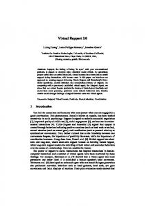
2.1 Contaminated sites According to the Swedish EPA (SEPA, 1999b), a contaminated site is defined as any site, landfill, area, groundwater or sediment that is contaminated from one or more local point sources to the extent that the concentrations substantially exceed the local or regional background concentrations.1 The high number of contaminated sites has a historical background in the industrial revolution, where new techniques and processes were developed without any knowledge regarding the health and environmental impact of various substances. The substances present at sites that are classified as contaminated, can typically be of a wide variety, see Table 2.1. SEPA (1995) classifies industrial branches into four general risk classes according to e.g. branch-typical processes, handling of material, raw material, waste products, and harmfulness. For example, the paper and pulp industry is placed in the highest risk class (1), and chemical laundries and dry cleaners in risk class 2. Such general lists and inventories are useful for the assessment of potential contaminants that may be present at a site. Humans and eco-systems are exposed to contaminants in several ways. The potential exposure pathways are considered when developing national generic guideline values for concentration of substances in soil. For example in Sweden, seven exposure pathways have been included in the human exposure model (SEPA, 1996b): direct intake of contaminated soil, dermal contact with contaminated soil and dust, inhalation of dust, inhalation of vapours, intake of contaminated drinking water, intake of vegetables grown on the site, and intake of fish from nearby surface water (Figure 2.1). However, e.g. swimming in 1

Other types of sites with a contamination potential, but that do not follow the definition by SEPA, have been investigated in the case studies as well.

7

J. Norrman

Table 2.1. Industries and related polluting substances. From ISO/FDIS (2003). TYPE OF INDUSTRY

TYPICAL CONTAMINANTS

Petroleum industry

Volatile aromatics: benzene, toluene, xylenes and ethylbenzene; alkanes C5 to C20, gasoline lubricants, methyl ethyl ketone, methyl tert-butyl ether, polyaromatic hydrocarbons, acid tars, Pb, As, B, Cr, Cu, Mo, Ni

Petrol stations and other Volatile aromatics: benzene, toluene, xylenes and ethylbenzene; alkanes sites for storage, C5 to C20, methyl ethyl ketone, methyl tert-butyl ether (MTBE), Pb treatment and handling of petrol, oil, and gas. Gasworks

Phenols and alicyclic phenols, polyaromatic hydrocarbons, volatile aromatics, cyanides, thiocyanates, ammonia, sulphur compounds

Asphalt and tar production and products

Volatile aromatics: benzene, toluene, xylenes; phenols, naphthalenes, polyaromatic hydrocarbons and other hydrocarbons

Wood, wood fibre and laminate industries

Toluene, xylene, trichloroethene, methyl methacrylate, other solvents

Impregnation of wood

Phenols, As, B, Cr, Cu, Hg, Sn, Zn, flourides, polyaromatic hydrocarbons, creosote, chlorophenols, pesticides, dinitrophenol, PCCD/F

Paper and pulp industry

Chlorophenols, organic solvents, metals

Printing industries

Chlorinated solvents, benzene, toluene, xylenes, acetone, isopropanol, other solvents, Ag, As, Cr, Cu, Hg, Pb, Sb, Zn

Foundries, metal works, etc.

Al, As, Cd, Cu, Cr, Fe, Mn, Ni, Pb, Sb, Zn, phenols, formaldehyde, acids, cyanates, carbamides, amines, B, Ba, Hg, Se, Sn

Metal industry

Al, B, Cd, Cu, Cr, Fe, Mn, Ni, Pb, Sn, Zn, fluorides, PCBs, PCTs, hydrocarbons, chlorinated hydrocarbons, solvents, glycols, turpentine, paraffins, cyanides, phosphorus, acids, ethers, silicates, polyaromatic hydrocarbons, Sb, As, Co

Galvanising industry

Solvents, Ag, As, Cd, Cr, Cu, Ni, Pb, Zn, cyanides, hydrocarbons

Manufacturing of paint, lacquer and enamel

Solvents: petrol, turpentine, volatile aromatics, alcohols, ketones, esters, glycol ethers and esters, chlorinated hydrocarbons, acrylamides; As, Cr, Cu, Cd, Pb, Zn, Sb, B, Ba, Co, Mn, Hg, Mo, Ni, Se

Rubber and synthetics industries

Volatile aromatics: benzene, toluene, xylene and ethylbenzene; chlorinated solvents, other solvents, butadiene, Sb, B, Cd, Cr, Hg, Pb, Se, Te, Zn

Textile and tanneries

Sulphides and sulphates, chlorophenols, solvents, cyanides, acids, Al, As, B, Cd, Co, Cr, Pb, alcohols, esters, ketones, xylenes

Chemical laundries and dry cleaners

Trichloroethene, tetrachloroethene, turpentine, carbon tetrachloride

Auto repair

Aliphatic hydrocarbons, volatile aromatics, polyaromatic hydrocarbons, styrene, chlorinated hydrocarbons, other solvents, amines, isocyanates, methyl tert-buthyl ether (MTBE), glycols, toluene di-isocyanate (TDI), Al, Cu, Pb

8


contaminated surface water or intake of products from grazing animals could also be included. In Sweden, exposure to eco-systems are considered both as on-site and off-site effects (SEPA, 1996b). The on-site effects are associated with the soil function, while the off-site effects are concerned with the protection of freshwater aquatic life and the aquatic life cycles in nearby surface water.

Soil →

CONTAMINATED SITE

Soil → Soil → (Outdoor) Dust → Soil → Uptake in vegetables → Soil → Vapour → Indoor air → Soil → Groundwater → Soil → Groundwater → Surface water →

Exposure processes Intake of soil Dermal contact with soil Inhalation of dust Intake of vegetables Inhalation of vapour

HUMANS

Transport processes

Intake of drinking water Intake of fish

Figure 2.1. Transport and exposure pathways included in the human exposure model, which together with an eco-system exposure model, is used for deriving the Swedish generic guideline values.

Typical contaminated sites are characterised by complex contamination situations with mixed composition of contaminants due to the long history of activities at many sites. Contaminants which have been in the soil for many years may be biologically and/or chemically altered and exhibit a different toxicity than newly applied substances, and the combined effect of varying contaminants on humans and eco-systems is difficult to predict. In addition, the natural geological and hydrogeological conditions at contaminated sites in urban areas are often disturbed by anthropogenic activities, i.e. excavation and redistribution of natural materials, presence of filling material from other sites, and installations such as pipes and drainage systems. Redistributed and filling materials are usually difficult to characterise due to the unknown content, and pipes and drains may

9

J. Norrman

cause water to flow in unexpected directions. At sites in rural areas, anthropogenic influences may be less significant and the geological and hydrogeological conditions relatively undisturbed. The exposure of humans and eco-systems to contaminants and the recipient to be protected vary from site to site, as does the economic and environmental value of protecting the recipients. The distribution of contaminants between soil particles, vapour and water, and the spread of contaminants to ground- and surface water are governed by site-specific conditions, e.g. type of contaminants present, soil type, soil material, soil water content, groundwater recharge, hydraulic conductivity and hydraulic gradient. A summary of typical factors to consider for the characterisation of contaminated sites is presented in Figure 2.2. For qualitative and quantitative prediction of the spread of contaminants from a site, an understanding of the governing processes and the models by which these are described is necessary. The following sections provide a brief introduction to flow and transport processes.

2.2 Transport processes In the following sections (2.2 – 2.4), additional references to those given in the text, are Fetter (1993) and Selker et al. (1999). Transport and dilution Groundwater flows as a result of differences in energy potential, from a high potential to a low potential, as summarised by Darcy’s law. Certain forces resist the movement of the fluid through the soil matrix: external forces or “friction”, and internal forces such as the viscosity of the fluid. The hydraulic conductivity, K [m/s], is a measure of the ability of water to flow through a specific medium, and is a parameter that combines both the characteristics of the medium (intrinsic permeability) and of the fluid itself, i.e. water. The basic transport processes are advection, dispersion and diffusion. Advection is the process by which moving groundwater carries solutes, and by which contaminants travel at the same rate as the average linear velocity of the groundwater.

10


?

CONTAMINATED SITE ? ?

? ?

? ? PROTECTED AREA

? ?

HOUSING

FACTORS:

ISSUES:

Site history

History of the industrial activity on site.

Contaminants

Contaminants present, properties, toxicity, amounts.

Exposure to humans

Land-use, accessibility to site, transport of contaminants.

Exposure to eco-systems

Recipients, vulnerable areas.

Geology

Geological history, soil material, anthropogenic activities, e.g. excavations.

Hydrology

Precipitation and evaporation, land surface and infiltration.

Hydrogeology

Geological history, transport conditions, anthropogenic activities, e.g. pipes and drains.

Physical boundaries

Geological units, hydrogeological boundaries, man-made boundaries.

Administrative boundaries

Landowner, environmental legislation, responsibility.

Time

Will conditions change over time?

Figure 2.2. Summary of typical factors to consider for the characterisation of contaminated sites.

Mechanical dispersion dilutes the solute as it is carried through the porous media. Dispersion along the streamline of fluid flow is called longitudinal dispersion, as opposed to lateral and vertical dispersion normal to the pathway of fluid flow, and is a microscopic level phenomenon. The velocity of fluid varies as fluid moves more quickly through the centre of a pore than along the edges (Figure 2.3a), where the maximum fluid velocity varies according to the size of the pore. In addition, because of the shape of the interconnected pore-space, some fluid travels in longer pathways than other fluid (Figure 2.3b). Thus, lateral and

11

J. Norrman

vertical dispersion are caused by flow paths splitting and branching out to the side. The mechanical dispersion is obtained by the combination of the average linear velocity and the dynamic dispersivity.

B

A Friction in pore

Long path

Short path Figure 2.3. Microscopic scale mechanical dispersion processes.

Diffusion causes molecules in areas of high concentration to move to areas of lower concentration, as described in Fick’s law. In porous media, diffusion will not be as fast as in free water because ions need to move round the grains blocking their passage. An effective diffusion coefficient is used for transport in groundwater, which is dependent on the tortuosity. Tortuosity is the actual length of the migration path divided by the straight-line distance between the ends of the path. Diffusion can take place even if the hydraulic gradient is zero, i.e. a solute can move in more or less still-standing water. Molecular diffusion and mechanical dispersion are together represented by hydrodynamic dispersion, since these two processes cannot be separated in flowing groundwater. The dominant process can be estimated by means of the Peclet number, which is a combination of the average linear velocity, the average particle diameter and the effective diffusion coefficient. In principle, the higher the velocities, the more dominant the dispersion processes and vice versa. Retardation and degradation There are two broad classes of solutes; conservative and reactive. Conservative solutes do not react with the aquifer material, nor do they degrade. Retardation of a reactive solute is caused by chemical and physical processes which slow down the solute movement. Reactive solutes interact with the soil by e.g. adsorption, i.e. charged ions in the water may be adsorbed to electrically charged surfaces. The adsorption can be in a weak form, resulting from the physical process caused by van der Waals forces, or in a stronger form, due to chemical bonding between

12


the surface and the ion. Adsorption is dependent on the amount of charged surfaces in the porous medium - clays, organic substances, iron-oxides and hydroxides, and aluminium oxides are especially rich in negatively charged surface positions. Positively charged surface positions are not as abundant, causing cations commonly to be more strongly adsorbed than anions. Adsorption of cations can be seen as a competition with protons for available negative surface positions, thus under acid conditions (i.e. many protons) cation adsorption is minimal, and anions may be adsorbed instead. Some substances are strongly influenced by the redox conditions: in general, reduced conditions increase the solubility of metals. Adsorption also depends on the size of the ion: smaller ions fit more easily than larger ions, and are in general more easily adsorbed. Adsorption is usually given as an isotherm when included in calculations. An isotherm is a graphical plot of the adsorbed mass per unit weight of soil as a function of the equilibrium concentration of the solute remaining in solution. There are three different types of physical adsorption models: the linear, the Freundlich and the Langmuir isotherm, see Figure 2.4. The linear isotherm is the most commonly used. Here, the relation between the adsorbed mass and the concentration of the solute is constant, i.e. all ions will distribute similarly between the soil particles and in the water. The constant distribution coefficient is usually referred to as Kd. However, the number of surface positions is in reality limited and therefore the two other models were developed to account for slower adsorption at higher concentrations. The Langmuir isotherm additionally takes the total concentration of surface positions into account. Isotherms are commonly fitted experimentally and the shape of the plot is not only dependent on the specific solute but on the actual material and any other species present. Groundwater usually contains several solutes, which during the transportation moves through porous or fractured media with different mineral surfaces and a varying organic content. Thus, the simplified Kd-concept can be rather misleading, see e.g. Bethke and Brady (2000). Surface complexation models are another way of describing the adsorption of inorganic species on mineral surfaces, see e.g. Dzombak and Morel (1990). The basic principles are: (1) adsorption takes place at surface-specific positions with varying electrical charges and different shapes and sizes; (2) adsorption reactions can be described quantitatively by equilibrium equations in the same way as for solutions; (3) The electrical charge of the surface is a result of adsorption reactions, i.e. the charge changes due to complexation; and (4) the effect of the electrically charged surface is included in the equilibrium equations. In general,

13

J. Norrman

this is a more detailed and accurate way of modelling adsorption. The uncertainties related to using complexation models are associated with the specification of the amount and properties of the adsorption substrates rather than the actual choice of model.

Concentration adsorbed

Freundlich isotherm Total concentration of sites Langmuir isotherm

Linear isotherm (Kd ) Concentration in solution

Figure 2.4. The linear, Freundlich and Langmuir isotherms.

In general, organic compounds are hydrophobic, i.e. they tend to partition into an organic phase such as octanol rather than into water. Hydrophobicity is measured by the octanol-water partition coefficient, KOW, which is the ratio of a compound’s concentration in the octanol phase to that in the aqueous phase. It is a good predictor of adsorption behaviour and bio-accumulation. High KOW values correspond to low solubility and tend to accumulate in fat, whereas low KOW values, correspond to high solubility and are in general more biodegradable. Because of their limited solubility, non-polar organic liquids often form a separate phase in the subsurface; such liquids are referred to as NAPLs (nonaqueous phase-liquids), see section 2.3. When dissolved in water, non-polar molecules tend to be attracted to surfaces that are less polar than water. There is a small but limited amount of adsorption of organics on pure mineral surfaces, but the primary adsorptive phase is the fraction of organic solids in the soil or aquifer. Dilution and retardation processes are mass-conserving, although causing a detainment of mass transport in time. Degradation processes, on the other hand, cause the total mass to decrease due to, for example, chemical and radioactive decay and biodegradation (Figure 2.5). Radio-nuclides will undergo radioactive

14


Concentration in solution

decay, both in the dissolved and the sorbed phase. The rate of decay is commonly measured as the half-life of the radio-nuclide. Micro-organisms require nutrients and electron acceptors (e.g. oxygen, nitrate, iron and sulphate) in order to degrade organic substances. The organic substance acts as an energy source for the organisms. In general, microbial degradation is faster in aerobic than in anaerobic environments. However, the rate is dependent on the specific contaminant. The microbial activity consumes electron acceptors while degrading the organic substances: this often causes different redox zones in shallow plumes contaminated by organic substances (Lovley et al., 1994; Vroblesky and Chapelle, 1994; Skubal et al., 2001), see Figure 2.6. The terminal electron accepting processes are oxic, nitrate- and Mn(IV)-reducing, Fe(III)-reducing, sulphatereducing, and methanogenic, ranging from aerobe to reduced conditions. Biodegradation can be modelled in the same way as radioactive decay by using half-life constants, which is a rather simplified approach.

(a) (c) (b) (d)

Distance Figure 2.5. Spreading of a solute slug (an instantaneous point injection) at time t1 due to advection, dispersion, and: (a) no retardation and no decay, (b) no retardation but decay, (c) retardation but no decay, and (d) retardation and decay.

Organic contaminant Methanogenic Direction of groundwater flow

Fe(III)reducing

Oxic

Sulphate-reducing Nitrate- and Mn(IV)-reducing

Figure 2.6. Principle of different redox zones in shallow plumes contaminated by organic substances. Aerobic processes take place along the fringes of the plume while anaerobic processes take place in the plume core.

15

J. Norrman

2.3 Multi-phase flow and transport The unsaturated zone

Pressure head

Water flow in the unsaturated zone is a multi-phase flow situation: two-phase flow with water and air. Unsaturated soils have a lower hydraulic conductivity than saturated soils, due to the fact that some pores are filled with air and the soil moisture travels only through the wetted cross-section of the pore space. In unsaturated flow, the pore water is under a negative pressure caused by surface tension, termed the capillary potential. It is a function of the volumetric water content of the soil, known as a soil-water retention curve, which is dependent on whether the soil has undergone wetting or drying (hysteresis), see Figure 2.7. In simple terms, the total soil moisture potential is the sum of the capillary and the gravitational potentials. The flow of water in the unsaturated (or vadose) zone is described by the Richards equation, where the unsaturated hydraulic conductivity is a function of the water content (or capillary potential). Solutes in soil water will be subject to mechanical dispersion and adsorption in the same way as solutes in the saturated zone. There are both equilibrium and nonequilibrium models of mass transport in the vadose zone.

Main drainage curve

Main wetting curve Water content Figure 2.7. A soil-water retention curve.

Preferential flow causes an acceleration of water and contaminant transport through unsaturated soil, and gives rise to a rate of flow which is highly variable within units of soil that are homogeneous on the meter scale. Macro-pores in the root-zone, due to plant roots, shrinkage cracks, animal burrows or soil

16


subsidence, forms preferential pathways for the movement of water and solute, both horizontally and vertically, causing short-circuiting of the infiltrating water as it moves faster through the macro-pores. For water to flow along these “large” open channels, capillary forces must not pull it into the finer surrounding pores. Thus, the flow is dependent on the water content of the surrounding pores. Macro-pore flow can occur under two conditions: the surrounding pores are already water filled, or the flow through the macro-pores exceeds the rate of loss to the surrounding soil. A second type of preferential flow, fingering, occurs when a uniformly infiltrating solute front is split downwards in “fingers”, due to instability caused by pore-scale permeability variations. Instability typically occurs when water enters dry, coarse-textured, and unstructured soils. Funneling is a third type of preferential flow in unsaturated stratified soil, where water tends to move in fine-sand layers on top of a sloping coarse-sand layer. When the water reaches the end of the layer, it can vertically percolate again, albeit in a concentrated volume. These preferential flow processes are governed by smallscale heterogeneities and the structure of the soil, and are usually difficult to predict by means of analytical or numerical models. Non-aqueous phase liquids Liquids that are immiscible with water are often called non-aqueous phase liquids. They may have densities greater than that of water (dense non-aqueous phase liquids, DNAPLs) or less than water (light non-aqueous phase liquids, LNAPLs). Two-phase flow occurs below the groundwater table with water and a DNAPL, whereas three-phase flow occurs in the unsaturated zone with air, water, and a NAPL. The flow is dependent on the densities, viscosities, and interfacial tensions of the liquids. In addition to dispersion and diffusion, compounds can undergo adsorption and degradation. The NAPL can partition into the air as a vapour phase, and it may be partially soluble in water leading to both a dissolved phase and a non-aqueous phase. Finally, NAPLs may consist of multiple compounds, implying that the properties of the fluid may change with time as some compounds dissolve in water. LNAPL travels vertically in the vadose zone and for large spills, the LNAPL eventually rests on top of the water table, see Figure 2.8 (top). The mobile LNAPL can further migrate in the vadose zone following the slope of the water table. If it is a small spill, only residuals will remain in the vadose zone, acting as a source of contamination in terms of vaporisation and dissolution in percolating water. The most widespread LNAPLs are petrol, diesel and kerosene. DNAPLs will travel vertically in the vadose zone under the influence of gravity. Fingering

17

J. Norrman

may occur when DNAPL migrates through a water-wet unsaturated zone. When the DNAPL reaches the groundwater table, it continues to migrate downwards, see Figure 2.8 (bottom). Once the percolating DNAPL reaches an impermeable layer, it can begin to move sideways, even in the absence of a hydraulic gradient, following the slope of the aquitard. DNAPLs can spread vertically and horizontally in fracture systems and are extremely unpredictable with regard to spreading (Kueper and McWhorter, 1991). Examples of DNAPLs are halogenated organic solvents such as trichloroethene (TCE) and 1,1,1trichloroethane (TCA), substituted aromatics, phthalates, PCB mixtures, coal and process tars, and some pesticides.

Spill area Residual LNAPL

Vadose zone

Pooled LNAPL Saturated zone

Direction of groundwater flow Spill area Residual DNAPL Vadose zone Saturated zone Pooled DNAPL

Dissolved DNAPL

Impermeable layer

Direction of groundwater flow

Figure 2.8. Principles of the transport of LNAPL (top) and DNAPL (bottom).

2.4 Heterogeneity and anisotropy A number of variables that influence the contaminant migration from a contaminated site, with regard to spatial and temporal variation, are summarised in Table 2.2.

18


Table 2.2. Variables influencing contaminant migration. Modified from Mackay (1990). VARIABLE

DISTRIBUTION Spatial

Temporal

Geological Aquifer and soil media

X

Form of porosity

X

Aquifer geometry

X

Low-permeability layers

X

Hydrogeological / Hydraulic Effective porosity

X

X

Hydraulic conductivity

X

X

Storage coefficient

X

X

Infiltration mechanisms

X

X

Discharge mechanisms

X

X

Surface water/aquifer interactions

X

X

Precipitation

X

X

Evapotranspiration

X

X

Surface flow distribution

X

X

Hydrological

Contaminants Advection

X

Hydrodynamic dispersion

X

Adsorption

X

Degradation

X

X

Contaminated fluid density

X

X

19

J. Norrman

Several variables are scale-dependent, e.g. the hydraulic conductivity at a small scale has a very large variation, although when the volume measured is sufficiently large, the variation is significantly less. The “sufficiently large volume” is commonly referred to as the representative elementary volume (REV) of a system; it is much larger than the grains of the porous medium, although smaller than the distance between similar regions. However, measurements are not always performed on a representative scale, and therefore large-scale predictions based on assumptions of homogeneity are likely to deviate from observations, unless the observations are large enough to incorporate many heterogeneities. Heterogeneities in geological materials originate from changes in time and space of factors governing geological processes, meaning that the properties of the geological media change spatially. Anisotropy means that the properties of the geological media change between directions. The concepts of heterogeneity and anisotropy are illustrated in Figure 2.9.

A

B

C

D

Figure 2.9. The concepts of heterogeneity and anisotropy: A) homogeneous isotropic material, B) homogeneous anisotropic material, C) heterogeneous isotropic material, and D) heterogeneous anisotropic material.

The impact of heterogeneity and anisotropy on transport predictions can be considerable. The processes that govern the transport of substances are on a much smaller scale than those of flow, thus transport is more strongly influenced by heterogeneity. This is described in the above sections which discuss the multiphase flow. Dispersion, diffusion, adsorption, and degradation in the saturated zone are also small-scale processes, thus influenced by small-scale heterogeneities. Predictions that incorporate the uncertainty associated with heterogeneity and measurements can be performed by stochastic calculations or simulations, which are important tools for risk analysis, see e.g. de Marsily et al. (1998).

20


Transport conditions at contaminated sites are thus dependent on the geological processes that formed the deposits and any other anthropogenic activities that may influence the hydrogeological conditions. For example, in Sweden the geology is characterised by Quaternary deposits directly overlying a Precambrian crystalline bedrock, thus with no significant zone of weathered rock, except for some sedimentary outliers. The glacial and post-glacial deposits have been reformed by isostatic uplift and subsequent wave-washing of the shores. The geological processes have formed a landscape that has somewhat varying geological and hydrogeological features: the composition of deposits varies due to the origin of the material; the thickness of deposits varies due to local topographic and surrounding conditions; and the surface configuration of deposits varies due to the specific processes, e.g. glacio-fluvial or glacial. The latitude of Sweden, sorts the country into a boreal forest climate with large seasonal changes in temperature. However, local variations such as sea currents, the distance to the coast and large lakes, as well as altitude, affect the temperature and the amount of precipitation, and consequently, the typical seasonal variation of the groundwater table (Fredén, 1994). As an aid for conceptualising typical settings of hydrogeological features, work has been done to characterise the settings in order to describe the diverse conditions (Stejmar Eklund, 2002; SEPA, 1999a). At contaminated sites however, the natural conditions are often disturbed by anthropogenic activities. The difficulty in characterising the transport conditions, especially at sites where the conditions have been disturbed, makes it even more important to consider the uncertainties pertaining to transport predictions and, consequently, to risk assessment.

21

J. Norrman

22

3. Theoretical starting points

3

THEORETICAL BACKGROUND

This chapter presents a classification of uncertainties and introduces the reader to decision theory, Bayesian decision analysis, data worth analysis and risk analysis, which form the theoretical setting for this thesis. The chapter ends with a short discussion on the theoretical basis of the used method and the chosen terminology.

3.1 Uncertainty Sources of uncertainty may vary, and some authors argue that the sources are important to distinguish, as the uncertain quantities should be treated differently when included in risk and policy analysis, e.g. NRC (1996). A typical distinction is that between aleatory and epistemic uncertainty. Aleatory uncertainty arises because of fundamental or inherent variability or randomness in natural phenomena, sometimes referred to as type 1 uncertainty. Epistemic uncertainty (epistemological or type 2 uncertainty), on the other hand, refers to the lack of knowledge about natural phenomena and can be related to statistical and modelling uncertainty. Statistical uncertainty arises because of a lack of data. Modelling uncertainty is due to: (1) uncertainty as to whether all factors that influence the model have been included, or (2) uncertainty as to how the model describes the relationship between these factors (Faber and Stewart, 2003).2 However, some different standpoints exists in relation to what the probabilities actually describe: the classical view versus the Bayesian view. Classical thinking defines probability and risk as true properties of nature, i.e. randomness is an objectively measurable phenomenon. The Bayesian approach considers probability as a subjective measure of uncertainty; it is a knowledge phenomenon and probability is an epistemological issue. According to Aven and Kvaløy (2002), the concept of probability in the Bayesian approach is used as the analyst’s measure of uncertainty or degree of belief.3 For example, the toss of a coin is not necessarily characterised by randomness: if we know the shape and 2

Nilsen and Aven (2003) points out another source of discrepancy in models, namely: deliberate simplifications introduced by the analyst, e.g. a trade-off between project economy and level of detail in modeling, or when the model is considered to serve its purpose sufficiently well for the problem to which it is applied, see further Paper III. 3 Of course, from a subjectivist point of view, there is only epistemic uncertainty and no aleatory uncertainty.

23

J. Norrman

weight of the coin, the distance, the strength of the person tossing it, the atmospheric conditions of the room, etc., we would be able to predict with certainty whether it would be heads or tails. The choice of approach determines what the probabilities in the analysis input and output express and also, as argued by Nilsen and Aven (2003), the definition of models and how to understand and deal with model uncertainty.

3.2 Introduction to decision theory In brief, decision theory deals with making decisions when faced with imperfect information: a decision may have several outcomes, each associated with a consequence commonly expressed in utilities.4 There is normative (or prescriptive) decision theory, which is about how decisions should be made, and descriptive theory, which concerns how decisions are made. Prescriptive tools are needed to provide guidance for dealing with new decision problems although they should rarely be seen as providing a true answer on how to act. Different decision models can be applied in normative theory, depending on the degree of knowledge available. Categorisation of decision situations according to the degree of knowledge follows that of economists (Baird, 1989; Hansson, 1991; Covello and Merkhofer, 1993). Certainty, or deterministic knowledge, is prevailing when the outcome of each decision alternative is perfectly known. Ignorance is characterised by a situation where we have no knowledge whatsoever about the probability of different outcomes, i.e. no probabilistic knowledge. Decisions under conditions of risk are characterised by each decision alternative having more than one possible outcome, and that the probability of each is known, i.e. complete probabilistic knowledge. Decisions under uncertainty are characterised by each decision alternative having more than one possible outcome, of which the probability is only partially known, i.e. incomplete probabilistic knowledge. The most common decision rule for decision-making under risk is to maximise the expected utility (EU), that is, the decision alternative that has the highest expected utility should be chosen. Theoretically, the decision alternatives and the 4

The utility of an outcome is a concept meaning the satisfaction, happiness or wellbeing of an outcome. The quantification of utilities is often done in monetary terms, although this may fail to reflect the true utility. Utilities are often decided based upon bidding games to reveal the decision-maker’s preferences, see e.g. Baird, (1989), Hansson (1991) or Jensen (2001).

24


probability and the utility of the different outcomes must be known in order to apply the EU decision rule correctly. In cases where we are unable to completely describe and quantify the probabilities or the utilities of the different outcomes, other decision rules may be more appropriate. Examples of other decision rules are: maxiprobability (the decision is made on the basis of the most probable outcome), minimax (choosing the alternative that has the lowest maximal regret), maximin (choosing the alternative with the best worst outcome) and maximax (choosing the alternative that includes the best outcomes), for more detailed information see e.g. Johannesson (1998) and Baird (1989).5 The necessary information for applying a specific decision rule is not always available, and in practice, decision-makers are often forced to make decisions under conditions of uncertainty and time constraints (Johannesson, 1998).

3.3 The normative decision process Keeney (1982; 1984) regards decision analysis as “a formalization of common sense for decision problems which are too complex for informal common sense.” Dakins et al. (1994) describes it as follows “Decision analysis is a technique to help organise and structure the decision maker’s thought process, elicit judgements from the decision maker or other experts, check for internal inconsistencies in the judgements, assist in bringing these judgements together into a coherent whole, and process the information and identify a best strategy for action”. Baird (1989) concludes that there are numerous different descriptions of the decision-making process, mostly starting with “formulating the goals” and ending with “implementing a course of action”. Hansson (1991) identifies three stages in the decision process: (1) identification of the problem, (2) development to define and clarify the options, and (3) selection of alternative. Keeney (1982) takes a more narrow approach, when discussing the methodology of decision analysis. He identifies four steps: (1) structure the decision problem, (2) assess the possible impacts of each alternative, (3) determine the preferences of decision makers, and (4) evaluate and compare alternatives. In practice, applying decision models to real world situations requires simplifications in order to be able to formulate a model. The above-mentioned steps are important for making sound simplifications and delimiting the problem. In this context, we do not only face uncertainties related to the physical world but 5

Under conditions of large scientific uncertainty, the precautionary principle is often said to be the foundation on which to base decision-making (Gollier and Treich, 2003).

25

J. Norrman

also uncertainties associated with our formulation and delimitation of the decision problem. Morgan and Henrion (1990) summarise several uncertain quantities included in policy analysis, with recommendations on how they should be treated. Table 3.1 has been slightly modified to fit the topic of this thesis. The decision variable (row 3) is a quantity describing what the action decided upon should achieve or aim to achieve. There is often a risk associated with each decision alternative, i.e. a probability of failing to meet the defined decision variable and the consequence of this. The strength of the summary by Morgan and Henrion (1990) is that it identifies which uncertainties are related to empirical quantities, to the decision-analyst’s choices, or to the decision-maker’s values or preferences, and how they can be treated in an analysis. Uncertainties related to the quantities listed in Table 3.1 are partly investigated in this thesis. Many of these uncertainties have more to do with the difficulty of defining the decision-problem, rather than any ability or inability to describe the outcome of a specific action. In that regard we will never face a decision-situation with complete probabilistic knowledge: we are always dependent on the decision analyst’s delimitation and definition of the decision problem.

3.4 Bayesian decision analysis Many authors refer to Bayesian decision analysis (e.g. Davis et al., 1972; Grosser and Goodman, 1985; Marin et al., 1989; Varis, 1997; Korving and Clemens, 2002) although Aven and Kvaløy (2002) argue that the understanding of Bayesian analysis varies a great deal among risk analysts. Hansson (1991) defines Bayesianism or Bayesian decision theory as expected utility theory with both subjective utilities and subjective probabilities and presents four principles that summarise the ideas of Bayesianism. (1) The Bayesian subject has a coherent set of probabilistic beliefs, i.e. in compliance with the mathematical laws of probability. (2) The Bayesian subject has a complete set of probabilistic beliefs, meaning that the subject is able to assign a probability to each proposition, often subjective probabilities. This means that Bayesian decision-making is always decision-making under risk, never under uncertainty or ignorance. (3) When faced with new evidence, the Bayesian subject changes her/his beliefs in accordance with her/his conditional probabilities, following Bayes’ rule.

26


Table 3.1. Types of quantities in policy models and how they can be treated. Modified from Morgan and Henrion (1990). TYPE OF QUANTITY

EXAMPLES

COMMENT & TREATMENT OF UNCERTAINTY

Empirical parameter or chance variable

Hydraulic conductivity

Well-specified variables, for which uncertainty can be expressed.

Efficiency of remediation technology Cost of remediation technology

Treatment: probabilistica), parametricb), or switchoverc).

Defined constant

Atomic weight, π, days in a year

Treatment: certain by definition

Decision variable

Guideline values for concentration of contaminants in soil or water

There is no true value, but appropriate or “good” values.

(Definition of failure or Remediation goals)

Value parameter

Treatment: Probabilistic, parametric or switchover. Discount rate Value of environmental quality Risk attitude

Index variable

Time period Compliance boundary

These represent aspects of the decision maker’s preferences. Treatment d): parametric or switchover. Used to identify a location in the spatial or temporal domain of a model. Treatment: certain by definition.

Model domain parameter

Spatial extent of transport model Level of detail in models, e.g. the grid size in transport models Time horizon

Outcome criterion

Net present value Utility

Should be chosen so that the model deals adequately with the full range of the system of interest, often a trade-off in model design. Treatment: parametric or switchover. Variables used to measure the desirability of possible outcomes. The quantities are deterministic or probabilistic according to how the input quantities are treated. Treatment: determined by treatment of its inputs.

a) The parameter or variable is assigned a probability distribution. b) The parameter is assigned a set of values and varied in the analysis. c) A value is found for the variable or parameter, at which the optimal decision changes. d) It is an important aspect to test different values in order to clarify how the decision maker’s preferences impact on the decision (Morgan and Henrion, 1990).

27

J. Norrman

We may differentiate between subjective and objective Bayesianism. Subjective Bayesianism states that as long as the updating of the subjective probabilities follows Bayes’ rule, there are no further requirements on how to choose the initial subjective probabilities. Objective Bayesianism, on the other hand, states that, given the available information, there is a unique admissible probability assignment, i.e. it states a subject-independent probability function. (4) Bayesianism states that the rational agent chooses the option with the highest expected utility. Bayesian statistics differs from classical statistics in that it includes all kinds of data, i.e. both objective (hard data) and subjective (soft data) information for making a prior estimate of the probability of a certain event. In fact, it requires a prior belief. By using Bayes’ theorem, the prior estimate is updated to posterior probabilities. The more hard data that are used to update the prior estimate, the more the updated information will reflect the collected hard data. The prior estimate may be solely based on subjective information, i.e. expert judgement. Decision analysis using the prior estimates of the probabilities of an event (or outcome) is called prior analysis. Updating the prior estimates and repeating the decision analysis is called posterior analysis (Faber and Stewart, 2003; Freeze et al., 1992).

3.5 The value of information or data worth analysis Apart from the fact that decision analysis provides insight into the different decision alternatives in a formalised manner, it also has another useful feature; by using Bayes’ theorem and the EU decision model, one can calculate the value of information, referred to as data worth analysis by some authors, e.g. Freeze et al. (1992). From a strictly decision-analytical perspective, information has no value if the data provided do not have the potential to change the best course of action.6 There are some commonly used concepts in data worth analysis: Expected Value of Perfect Information (EVPI), Expected Value of Including Uncertainty (EVIU), Value of Information (VOI), Expected Value of Information (EVI), and Expected Value of Sample Information (EVSI).

6

This idea of data worth may sometimes be questionable. Is more knowledge about the decision situation really of no worth, even if it does not change our actions? McDaniels and Gregory (2004) presented the concept of Value of Learning as a an addition to the Value of Information concept and included it in decision analysis. This concept is not treated in this thesis.

28


The concept of EVPI is an estimation of the maximum amount one should pay for additional information before taking the actual decision. In words, it can be described as the expected value of the optimal decision with perfect information, minus the expected value of the decision without perfect information. Obviously, perfect information is not available; instead the expected value of each available option is weighted with the probability that it is the optimal decision. This is described by e.g. Keeney (1982), Baird (1989), Morgan and Henrion (1990), Dakins et al. (1994), Hammitt and Shlyakhter (1999), and Back (2003), and treated in Paper V and VI. While EVPI compares the expected value of Bayes’ decision with a decision made with access to perfect information, EVIU compares Bayes’ decision with a decision where uncertainty is ignored. This is described by e.g. Morgan and Henrion (1990) and Dakins et al. (1994). The other terms listed above, VOI, EVI, and EVSI, all describe the same concept, which relates to the analysis of whether the incremental value of a decision, when uncertainty is reduced due to additional information, is greater than the cost of obtaining this information. Thus, the critical issue is not the degree to which uncertainty will be reduced or the value of that reduction in itself. The value of this information must hence be calculated before collecting it in order to decide whether or not it is worthwhile. The analysis carried out using the estimate of what information additional data will provide, before actually collecting the data, is called the pre-posterior analysis due to the fact that it involves the possible posterior distributions resulting from potential samples not yet taken (Baird, 1989; Freeze et al., 1992; Faber and Stewart, 2003). Faber and Stewart (2003) argue that the concept of pre-posterior analysis is presently underutilised. One reason may be the difficulty in estimating the information that can be expected from sampling. Suggested methods are given by e.g. Freeze et al. (1992), James and Freeze (1993), Dakins et al. (1996) and Back (2003).

3.6 Risk analysis The main objective of performing risk analysis is, according to Nilsen and Aven (2003), to support decision-making processes and provide a basis for comparing alternative concepts, actions or system configurations under uncertainty. Risk is defined in different ways for specific purposes and in the context of engineering decision-making, and Faber and Stewart (2003) argue that it is important to be precise and consistent in our understanding of risk. Typically, risk is defined as the expected consequences of a given activity. In its simplest form, risk (R) is then defined as the probability (P) of an activity that is associated with only one

29

J. Norrman

event, multiplied by its consequences (C) given that this event occurs. 7 If C is expressed as a cost or utility, the risk is thus the expected cost or utility of a given event. This is the definition of risk that is used throughout this thesis: R=P×C The National Research Council (NRC, 1996) identifies two fundamental phases of risk analysis, namely risk assessment and risk management. Covello and Merkhofer (1993) on the other hand, separates risk analysis and risk management and holds that risk analysis provides key information for the risk management process, see Figure 3.1. Regardless of whether risk management is placed within or outside risk analysis, it considers the social, economic and political factors involved in the decision-making process and determines the acceptability of damage and what, if any, action should be taken. The process of risk management as suggested by Covello and Merkhofer (1993), follows in principle the methodology of decision analysis as presented by Keeney (1982), see Figure 3.1. Risk assessment on the other hand, is a set of analytical techniques for answering the question: How much damage or injury can be expected as a result of a specific event? A committee of the National Academy of Sciences devised a formulation of risk assessment as a four-step process: (1) hazard identification, (2) doseresponse assessment, (3) exposure assessment, and (4) risk characterisation, see Figure 3.1.8 Covello and Merkhofer (1993) defines risk assessment slightly differently, placing hazard identification outside of risk assessment, which instead consists of: (1) release assessment, (2) exposure assessment, (3) consequence assessment, and (4) risk estimation, see Figure 3.1. In both definitions, the fourth step - risk characterisation or risk estimation - aims at integrating the results from the previous steps. Possibly, the suggested definition of risk analysis by Covello and Merkhofer (1993) is more useful if risk is, as is usually the case, seen as the sum of the links in a risk chain consisting of 1) risk source release processes, 2) exposure processes, and 3) consequence processes. For a risk to exist, this chain must remain unbroken. This thesis does not present in-depth quantitative risk assessment regarding dose-response assessment or consequence assessment, but

7

In its extreme, the simplest definition of risk is the probability of an unwanted event. Called “the Red Book”, written by the National Research Council of the Academy of Sciences in 1983 (Felter et al., 1998; Asante-Duah, 1998; Covello and Merkhofer, 1993; NRC, 1996; Davies, 1996).

8

30


follows the view of risk as a chain of events, for further information please see sections 5.2, 5.3 and 5.4.

Phases of Risk Analysis according to NRC, 1996. RISK ANALYSIS Risk Assessment Hazard identification Dose-response assessment

Exposure assessment Risk characterisation

Risk Management

Stages of Risk Analysis and its relation to Risk Management according to Covello and Merkhofer, 1993. RISK ANALYSIS Hazard identification

Risk assessment Release assessment Consequence assessment Exposure assessment Risk estimation

Risk evaluation

Risk information

RISK MANAGEMENT Generate options

Option evaluation

Option selection

Implementation and enforcement

Methodology of Decision Analysis according to Keeney, 1982. DECISION ANALYSIS Structure the decision problem

Assess the possible impacts of each alternative

Determine preferences of decision-makers

Evaluate and compare alternatives

Figure 3.1. The definition of risk analysis presented by NRC (1996) and Covello and Merkhofer (1993) are different. The risk analysis presented by NRC (1996) includes risk management, whereas Covello and Merkhofer (1993) separates this from the risk analysis phase. The methodology of decision analysis presented by Keeney (1982) is similar to that of risk management as proposed by Covello and Merkhofer (1993).

31

J. Norrman

3.7 Starting points and terminology used The main objective of this thesis is to develop, apply and evaluate an approach based on decision analysis for handling uncertainties and evaluating alternative actions at contaminated sites. Obviously, normative decision analysis is used to achieve this. The EU decision criterion is used in this thesis, with the utilities expressed exclusively in monetary terms. Thus, the outcome of each decision alternative will be expressed as a total expected value rather than as the expected utility. The total expected value includes the costs and benefits associated with the implementation of the alternative and the expected cost of failing to meet the defined decision variable (or as it is called here, the failure criterion). This failure cost however, is not viewed as being subjective, but rather as uncertain or unknown. Only individual decision makers are considered and the decisionmaker is assumed to be risk-neutral. However, as will be discussed in section 5.10, there may exist an acceptable risk by which the decision model becomes constrained. Choosing strategies for environmental protection or remediation are decision problems that are never characterised by deterministic knowledge, nor by complete ignorance, since the foundation lies in the physical nature of the site in question. Decisions under risk imply that we are able to quantify the probabilities of the different outcomes of the alternative strategies, while decisions under uncertainty imply that there is some uncertainty connected to these probabilities (second order uncertainty). The view of uncertainty adopted in this thesis is primarily a subjective Bayesian view, meaning that a probability is a function not only of the event, but also of the relevant information known to the analyst. Consequently, by applying a Bayesian approach, we are assuming conditions under risk. The term risk analysis is used in a variety of ways and it is consciously avoided here. Instead, referring to Bayesian decision analysis, makes the main objective clearer, that is, the aim of supporting decision-making - although it may not be obvious to someone unfamiliar with decision theory that the decisions considered always are made under risk.

32

4. General working approach

4

GENERAL WORKING APPROACH

This chapter starts with a presentation of the general project life cycle of remediation projects as described by the Swedish EPA. The participants in the projects are introduced and their respective roles and perspectives discussed. Finally, key issues on communication within remediation projects are described.

4.1 Phases of the general remediation project The implementation of projects for investigating and possibly remediating contaminated sites, which are publicly funded, is divided into six phases by the Swedish EPA (SEPA, 1997b): •

Initiation,

•

Preliminary study,

•

Main study,

•

Preparations,

•

Implementation, and

•

Follow up.

The structure is also applicable to privately funded projects. The most important issues and decisions from the perspective of SEPA (1997b) are summarised in Table 4.1. The end of each phase is a decision of the “go to next phase” or “stop” type. Apart from these general decisions, there are several others of a more technical nature within the phases, e.g. how the sampling should be performed or what type of remediation measures should be implemented.

4.2 The participants and their perspectives Remediation projects may be initiated by different stakeholders, each with their own perspective on the problem at hand. Private companies, public companies or municipalities may see benefits in investigating sites suspected of being contaminated, or in order to exploit land. A regulatory agency may order an

33

J. Norrman

Table 4.1. Summary of activities, questions to be investigated, and decisions to be made during project phases based on the current approach (SEPA, 1997b). PHASE AND MAIN ACTIVITIES

MAIN QUESTIONS TO BE INVESTIGATED

MAIN DECISION OPTIONS

1. INITIATION

Contamination potential, spreading and spreading possibilities, effects, and risks are in general evaluated by a desk study.

Obtain more data (Preliminary study or Main study)

The magnitude of the problem and need of resources.

Remediation

Responsibility for and financing of continued investigations (and possibly remediation).

No action - STOP

Desk study Problem identification

2. PRELIMINARY STUDY Desk study Risk classification Preliminary investigation Responsibility invest. 3. MAIN STUDY Detailed investigation Risk assessment Responsibility invest. Remediation alternatives investigation Risk valuation

Preliminary assessment of health and environmental risks. Obtain more data (Main study) The need for investigations. Remediation Responsibility for and financing of continued investigations and remediation. No action - STOP Public information. Detailed assessment of health risks and environmental risks. Measurable goals for the remediation of the site. Suitable remediation method and future main actor. Need for permission, permits and similar. Suitable form for implementation of the remediation.

Remediation No action - STOP (If more data are needed, the Main study is continued until there are sufficient data)

Public information.

Remediation investigation 4. PREPARATIONS Program preparation Permit applications Contractor tender

Design and planning of remediation measures and possibly formulation of tender documentation for contractors.

(Investment decisions)

Application for permission and permits etc, and reports to regulatory agencies. Environmental inspection before implementation of remediation measures. Inspection by regulatory agencies. Public information.

5. IMPLEMENTATION

Implementation by a contractor or the responsible party.

Remediation works

Environmental inspection during the implementation of remediation.

Environmental inspection Documentation of the work performed 6. FOLLOW UP Inspection Evaluation Feedback

(Authorisation of the implementation)

Inspection by regulatory agencies. Public information. Environmental inspection and evaluation of fulfilment of remediation goals. Authorisation by regulatory agencies. Guarantee inspection. Public information.

Authorisation - STOP Continue inspection program Change inspection program Additional remediation

34


investigation when a site is suspected of being contaminated.9 More rarely, environmental impact on the surroundings may indicate contamination and force a regulatory agency to initiate a project. There are several participants connected to the phases of the general project life cycle depending on how the contractor’s contract is written. For a general contract (utförandeentreprenad), see Figure 4.1 and for a design and construction contract (totalentreprenad), see Figure 4.2.

Technical support

SITE-OWNER

Technical consultant

INVESTIGATIONS

PREPARATIONS

Preliminary study

Main study

Consultant

Consultant

Preparations for implementation Group of consultants

Management for direction of works Administrative consultant

IMPLEMENTATION Implementation Inspection Contractor Control during implementation Consultant or group of consultants

COMMUNICATION, AUTHORISATION & CONTROL THROUGHOUT PROJECT

REGULATORY AGENCY Figure 4.1. Participants involved in the phases of a general contract project (used with the permission of Blom, 2004). The colour green is associated with the site-owner’s organisation, which may be either public or private. The pale yellow colour refers to the consultants involved, while blue indicates the contractor.

9

By a regulatory agency is meant the (Swedish) authorities that exercise supervisory powers with the view to ensuring that the bodies it monitors observe the law and existing guidelines for protecting the environment and public health, at a regional and local level. In Sweden, these authorities are the county administrations and the municipalities. The Swedish EPA is a central environmental authority with the main task to promote environmental work on both a national and international level.

35

J. Norrman

Technical support

SITE-OWNER

Management for direction of works Administrative consultant

Technical consultant

PREPREPARATIONS

INVESTIGATIONS Preliminary study Consultant

Main study Consultant

Preparations for design and construct contract Group of consultants

PREPARATIONS AND IMPLEMENTATION Preparations for implementation Consultant group of the contractor

Implementation Inspection Contractor

Inspection during implementation Consultant or group of consultants COMMUNICATION, AUTHORISATION & CONTROL THROUGHOUT PROJECT

REGULATORY AGENCY Figure 4.2. Participants involved in the project phases for a design and construction contract (used with the permission of Blom, 2004). The colour green is associated with the siteowner’s organisation, which may be either public or private. The pale yellow colour refers to the consultants involved, while blue indicates the contractor.

Table 4.2 provides an overview of the participants and other actors and their typical benefits, costs and economic risks in remediation projects. However, these should be seen as typical participants and actors with typical perspectives. In reality, the incentives of one type of participant or actor may differ greatly. Additionally, the roles may be combined, e.g. a private problem-owner may also be the one who carries out the actual remediation work. Regulatory agencies should apply regulations to ensure a sustainable economic growth while protecting the environment and public health. Funding authorities should distribute their budgeted grants in a cost effective manner with attention to the environmental benefit they provide.10 The demand for societal cost- efficiency in sustainability and inter-generation equity perspectives has legal force due to being enshrined in environmental legislation. For a private project financier, the 10

By a funding authority is meant authorities that provide public resources to investigate and remediate sites where no responsible part is found. In Sweden, the Swedish EPA distributes money to the county administrations, which in turn distribute them to the municipalities, or run the projects themselves at sites where they are appointed to be the responsible part.

36


preferences may be different, usually cost-benefit within shorter time frames or fulfilling duties in compliance with environmental legislation.

4.3 Risk valuation and communication The risk valuation is identified as a part of the Main study and is a process of weighing the environmental, economic and technical aspects together in order to reach a cost-efficient decision on the remediation measures. Projects concerned with remediating contaminated sites are typically associated with large uncertainties regarding the remediation goals, goals which are usually agreed in co-operation with the regulatory agency. The risk valuation and the remediation goals are connected, since the remediation goals dictate the remediation efforts and these efforts are then included in the risk valuation process. The valuation and consequently, the decisions should be made by the site-owner in agreement with the regulatory agency, whereas the task of supplying the site-owner with information for making decisions in each project phase is performed by consultants. Obviously, the data provided by the site-owner’s organisation must be transparent and traceable in order to ensure a good communication with the regulatory agency. In Sweden, regulatory agencies still have relatively limited experience of how to regulate risks and how to use soil or other guideline values in combination with reasonable expenditure and the available technical possibilities. This has resulted in sites lying fallow while waiting for clearance from regulatory agencies on how to proceed, as a consequence, incurring unnecessary costs. The site-owner, on the other hand, is often not in a position to determine the data required, nor is she/he well-informed about the available options (de Mulder and Kooijman, 2003; Moorhouse and Millet, 1994). Thus, it is important that the consultant is in a position to inform the site-owner about the options and requirements and to provide information useful for decision-making to their client, by extension, to the regulatory agency.11

11

The ability to inform the site-owner is not only dependent on the consultant: some consultants have experienced that site-owners prefer not to know the details.

37

J. Norrman

Table 4.2. Participants and actors and their perspectives. Example from Sweden. PARTICIPANT / ACTOR

REGULATORY AGENCY FUNDING AUTHORITY

PUBLIC SITE-OWNER

Organisation.

County Administration, Municipality a)

Swedish EPA, County Administration

Municipality

Benefits of carrying out a remediation project.

A safe environment and a healthy population.

A safe environment and a healthy population.

Knowledge capacity building.

Knowledge capacity building.

Local good-will, political good-will, more efficient landuse, more people in the municipality, better local environment, improved public health.

Costs for carrying out a remediation project.

Labour costs for administration, inspection and follow up b).

Labour costs for administration Labour costs for administraof applications and follow up b). tion and (today) 10% of total project cost. 90% is funded.

Trade-off or type of decision.

Apply environmental regulations that are costefficient.

1. Prioritising between objects.

Main uncertainties affecting the decision.

What are the true environmental and health effects of applying a certain remediation goal or guideline value?

1. Are the worst objects included?

Consequences and economical risks of a nonoptimal decision.

-) Loss of environmental values, increased public health care costs, loss of good-will, future reinvestigations at the site.

-) Loss of environmental values, increased public health care costs, loss of good-will, bad publicity, future reinvestigations at the site.

-) Decisions too risky +) Decisions too conservative

Data or input to improve decisions.

a) b)

38

Meeting the remediation goals within the approved 2. Approving budgets for priori- budget. or tised sites that are costProactive: reaching higher efficient. than regulations due to expected economic profit.

2. What are the true environmental and health effects of applying a certain remediation goal or guideline value?

+) Unnecessary land use +) Resources spent on areas restrictions, too heavy where they were not needed. economic burden on the site-owner, less economic growth.

Site-specific conditions such as e.g.: contaminants, soil conditions, spreading conditions, volumes, concentrations.

Depending on how the contract is written. -) Loss of environmental values, additional remediation costs in the short and long term, increased public health care costs, loss of good-will, bad publicity. +) Unnecessary investigation and/or remediation costs.

Communication between stakeholders on risks, costs and benefits.

Communication between stakeholders on risks, costs and benefits.

Communication with the regulatory agency on risks, costs and benefits.

General data, e.g. monitoring data, epidemiological data, toxicological data, improved risk assessment, knowledge capacity building.

1. Better site information.

More site-specific data e.g.: contaminants, soil conditions, spreading conditions, volumes, concentrations.

2. General data, e.g. monitoring data, epidemiological data, toxicological data, improved risk assessment, knowledge capacity building.

The Swedish EPA only acts as an advisory authority and offers guidelines for inspection. Labour costs of regulatory agencies and funding authorities do not usually appear in the total project budget.


Table 4.2. continued… PRIVATE SITE-OWNER

CONSULTANCY AGENCIES

CONTRACTOR

Private companies or individuals

Private and public companies

Private companies

Economic gain due to e.g. more efficient land-use, better insurance, better loans, good-will from clients, no environmental debt in booking.

Economic gain to company due to work assignment, knowledge capacity building, additional experience, client good-will.

Economic gain to company due to work assignment, knowledge capacity building, additional experience, client good-will.

An improved living environment and improved health.

100% of total project cost.

-

-

Possibly reduced value of properties or loss of work opportunities.

Meeting the remediation goals as cheaply as possible. or

Suggesting how to carry out the assignment in order to meet the goals.

Suggesting how to carry out the assignment in order to meet the goals.

“For or against” a remediation project.

Proactive: reaching higher than regulations due to expected economic profit.

Quality of work against economic profit.

Quality of work against economic profit.




-

Depending on how contract is formulated.



-) Health effects, environmental effects.

-) Loss of good-will, additional short and long term remediation costs, penalties.

-) Additional work, liability costs.

-) Additional work, liability costs.

-) Decreased property values.

+) Unnecessary labour and material costs.

+) Unnecessary labour and material costs.

+) If the site-owner is public: possibly reduced budget for other facilities in the municipality.

Knowledge capacity building for personnel and communication with siteowner and contractor.

Knowledge capacity building for personnel and communication with siteowner and consultant.

-

+) Unnecessary investigation and/or remediation costs. Communication of risks, costs and benefits to the regulatory agency. More site-specific data e.g.: contaminants, soil conditions, spreading conditions, volumes, concentrations.

THE PUBLIC and NGOs

Increased land availability.

39

J. Norrman

Discussions and seminars at a conference in Spa 2001 (Rosenbaum and Turner, 2003) in relation to the role of geoscientists identified the need to bridge the gap between the providers of geo-information (in this case: the consultants and the contractors) and the end-users (in this case: the site-owner and the regulatory agency). Thus, an important issue for geoscientists today is not only to have knowledge about geoscience but also to understand the needs of the end-user and be able to communicate specific information, i.e. to provide relevant “decision information”. D'Agnese and O'Brien (2003) points out however, that the providers are often limited by their incomplete understanding of the decision process. In other words, it is common for consultants to deliver a complete solution rather than an informative document for decision-making to the siteowner. D'Agnese and O'Brien (2003) introduced the “Geoscience Knowledge Integration Paradigm” as a practical extension of the data and information integration achievements of the late 20th century. This is a consequence of the fact that providing data and information is no longer sufficient, as society now demands knowledge and wisdom to be explicitly packaged and disseminated for use in informed decision-making. The authors identify an increasing demand for user-specific solutions that contain clearly documented levels of uncertainty to be used by society to make operational decisions. The “Geoscience Knowledge Integration Paradigm” as a progression from data to wisdom takes the form a pyramid, Figure 4.3. Decision Making Decision Analysis Decision Information Knowledge Management and Application

Wisdom

Process Models, Predictive Models, Workflow Management, Protocols

Knowledge Process-Expertise Information Data

Geographic Information Systems, Data Archives, Data Warehouse, National Databases

The Geoscience Knowledge Integration Paradigm

Figure 4.3. The Geoscience Knowledge Integration Paradigm (D'Agnese and O'Brien, 2003).

40

5. Decision framework

5

DECISION FRAMEWORK

This chapter presents the decision framework that resulted from this thesis. In addition, examples of some critical issues that could benefit from using the approach are listed. This chapter also describes the main features of each part in the decision framework. Although there are a large number of tools and methods available, each suitable for different types of analyses, only the main ideas, some general methods and the tools that have been used during the doctoral project work will be summarised here, together with some selected tools that are believed to be of interest.

5.1 The proposed decision framework The main question in any remediation project, is whether or not the site should be remediated, although there are alternative actions, i.e. to perform field investigations or to monitor the site. This decision is not only dependent on the environmental and public health risks, but also on the available technology and the actual remediation cost. There is a trade-off between the level of risk society is willing to accept and the cost of reducing the risk. Using a decision analytical perspective means that this trade-off, or the risk valuation, is in focus from the very start of a project. The general project life cycle structure as presented by the Swedish EPA is used as a basis in this thesis. The structure is logical and wellsuited as a starting point for describing how to incorporate a decision analytical perspective in contaminated site remediation projects. The general project structure within a decision analytical perspective is presented in Figure 5.1, which aims to illustrate how the proposed approach relates to the general project life cycle. The project phases Initiation, Preliminary study, and Main study, are replaced by an iterative loop including a data worth analysis. The prior and posterior analyses, in Figure 5.1, include the decision analysis, and the pre-posterior analysis includes the data worth analysis. The decision-analytical approach includes both economical considerations and the technical and economic risks associated with each alternative action. It is related to the work normally performed by consultants involved in the investigation - and possibly pre-preparation - phases of a project, and works according the principle of iterative refinement of data and information. The main difference with regard to

41

J. Norrman

the general working approach is that all factors relevant to the decision are included in each iteration. That is, besides the site-specific data, e.g. the decision variable and the remediation alternatives are included from the outset.

1, 2, 3. Prior analysis Estimation of the total expected value of each alternative action at the site by including costs, benefits and environmental risks, using available information. Pre-posterior analysis Are more data likely to be cost-effective?

Yes

Obtain more data

Posterior analysis Update the total expected value of each decision alternative using new data.

No

Choose the remediation alternative with the highest total expected value.

No action

Remediation

4. Preparation 5. Implementation 6. Follow Up

Authorisation

STOP (completion)

Figure 5.1. Project phases with a decision analytical approach included. The boxes within the dotted grey line are shown more in detail in Figure 5.2.

The proposed decision framework of this thesis is presented in Figure 5.2, and is a result of the case study applications (Papers I – VI). It excludes the last three phases of the general project life cycle, but shows the parts within the dotted grey line in Figure 5.1 in more detail. The framework outlined starts by delimiting the decision-problem, which here includes identifying the remediation goals. The remediation goals may be seen as the decision variable or the attribute against which all alternative actions are measured. The risk is constituted by failing to meet the remediation goals (section 5.2). By structuring the problem, the risk is further conceptualised for allowing it to be quantified (section 5.3). The available

42


data can be of any type: desk studies, inventories, experience, interviews and field investigations.

Existing data

PROBLEM IDENTIFICATION

Expert judgement

PROBLEM STRUCTURING

IDENTIFICATION OF ALTERNATIVES

CONCEPTUAL MODELS

PARAMETER UNCERTAINTY MODEL

PROBABILITY MODEL

CONSEQUENCE MODEL

DECISION MODEL

DECISION ANALYSIS

DATA WORTH ANALYSIS

DATA COLLECTION

NO MORE DATA

Decision Figure 5.2. The proposed decision framework and its sub-parts. In principle, it relates to the general project phases 1, 2 and 3, where the possible outcome of each iteration is: Obtain more data (data collection), or a decision on “No action” or “Remediation”.

43

J. Norrman

The next step is to identify possible alternative actions at the site together with the implementation cost for each of them (section 5.4). To account for uncertainties associated with failing to meet the defined decision variable, the approach includes the formulation of a quantitative probability model for the prediction of the probability of failure for each alternative action (sections 5.5 – 5.7). For a full quantification of the risk, the costs associated with the consequences of failing to meet the defined decision variable must be estimated (section 5.8). At this stage, the decision model for calculating the total expected value for each alternative action, is built (section 5.9). In the following decision analysis, the criterion of choosing the alternative with the highest total expected value assumes risk-neutrality. However, an important purpose of decision analysis is to use it as a basis for communication rather than as a strict rule for which alternative to choose. It is thus important to investigate which factors most affect the outcome of the analysis, i.e. performing a sensitivity analysis (section 5.10). The last stage, data worth analysis, contains the assessment of whether additional data are costeffective in relation to the decision to be made. This information can be obtained either quantitatively or qualitatively (section 5.11). The proposed decision framework in its final form has been applied in Papers III, IV, and VI, each of which presents case-specific input to the framework. The approach is used in Papers I and II, but is not as explicitly structured. Examples of critical issues in a typical remediation project, which are believed to benefit from using the proposed approach in terms of communicating, structuring and analysing information, are summarised in Table 5.1. The other phases of the general project life cycle, Preparation, Implementation, and Follow-up, are not included in the proposed decision framework. The decided actions are planned in the Preparation phase, thus the decisions in this case are e.g. what type of contractor should be chosen? During the Implementation phase, the contractor must fulfil the established remediation goals at a certain level of confidence. There are several possible detailed level decision situations for the contractor, e.g.: “Should we excavate this soil volume or not?”, “Should there be two or three extraction wells installed?”. These are decisions where optimisation techniques may be more appropriate, since the remediation strategy is already decided upon and the detailed implementation must be optimised within the constraints of a contract budget (Freeze and Gorelick, 1999). During the Follow-up phase, the decision should be made to

44


authorise the site, or to continue or change the inspection program.12 The Inspection phase is not treated as an independent part in the decision framework but included in some of the decision models (Papers V and VI).

Table 5.1. Examples of critical issues that are believed to benefit from the proposed approach. PROJECT PHASE

TYPICAL FEATURES

CRITICAL ISSUES

1. INITIATION

Desk study

How to formalise the use of soft data and expert judgement.

Soft data only Large uncertainties Low budget 2. PRELIMINARY STUDY

Desk study Field investigations Limited hard data Large uncertainties Budget constraints

3. MAIN STUDY

Detailed field investigations Remediation alternative assessment Risk valuation Hard data Uncertainties

How to treat large uncertainties. How to evaluate the cost-effectiveness of planned investigations. How to formalise the use of soft data and expert judgement combined with hard data. How to treat large uncertainties. How to evaluate the cost-effectiveness of planned investigations: type of investigation, type of medium to sample, type of analysis. How to evaluate the cost-effectiveness of planned investigations: type of investigation, type of medium to sample, type of analyses, number of samples, and location of samples. How to evaluate the cost-effectiveness of possible remediation alternatives: extent of remediation, type of remediation technique, efficiency and riskreducing effect of remediation techniques, costs, and consequences of an unsuccessful or insufficient remediation.

Budget constraints

12

The term monitoring is not used due to the impression of an on-going activity. The Follow-up phase should rather be seen as the final phase of a remediation project where the aim is to complete the project.

45

J. Norrman

5.2 Problem identification During the problem identification stage, the problem domain is defined, i.e. the failure criterion, the risk objects and the receptors. The failure criterion, or the decision variable, is the formulation of an attribute against which the decision alternatives can be compared, in terms of how well each alternative is expected to fulfil the criterion, the consequences if it does not, and the implementation cost of each alternative. The risk objects are the potential sources of contamination, and the receptors are the objects which to protect. One of the main features of the proposed approach is that it is problem-oriented, thus the desired outcome of the decision is in focus from the start. Morgan and Henrion (1990) point out that setting the boundaries for quantitative policy analysis is an iterative process of refining the formulation of the analysis and clarifying the questions to be addressed. Thus, it is important to recognise that the parts within the framework are interconnected and the boundaries and the definition of failure may be changed at any stage of the work, see Figure 5.3.13 Only single-attribute formulation of the decision problem has been studied in the proposed approach, referred to as the failure criterion, and the objective is to maximise the expected value of the decision for reaching this criterion.14 The failure criterion can apply at different points, in other words, the receptor be identified differently. One example is that, in a human health risk assessment, an explicit formulation such as ‘that not more than 1 person out of a population of 100,000 develops cancer’ is accepted - the population being the receptor. Another example is a criterion where the surrounding environment is the receptor, e.g. ‘no contamination is accepted off-site’, which is commonly used for the construction of waste disposal sites in Europe. The description of the consequences of the two examples, is obviously very different and the choice of failure criterion is dependent on the chosen boundaries of the analysis. In the proposed approach, the risk is the probability of exceeding the failure criterion multiplied by the consequences of exceeding the criterion. In the case studies analysed, the failure criteria employed are formulated on the basis of guideline values and environmental standards, but also in more general terms, e.g. not to increase the contaminant load above present day values. The failure criteria used in the case studies are summarised in Chapter 6. 13

For example, Keeney (1982) includes both the generation of decision alternatives and the specification of the objectives and attributes in the first phase of decision analysis (see Figure 3.1), and stresses the iterative nature of this phase. 14 An important issue is multi-attribute decision problems and the ability of decision analysis to provide a tool for this, although not treated here.

46


PROBLEM IDENTIFICATION

Existing data Expert judgement

PROBLEM STRUCTURING

IDENTIFICATION OF ALTERNATIVES CONSEQUENCE MODEL

CONCEPTUAL MODELS


PROBABILITY MODEL

Figure 5.3. The iterative nature of the parts of the general decision framework in which the problem is defined, structured, and conceptualised.

The result of the problem identification stage is highly dependent on the individuals who are defining the boundaries and the failure criterion. Thus, it is important to have as much relevant information as possible and to assemble a group of persons who are well-acquainted with the problem, in addition to at least one person who is familiar with decision-analytical approaches.

5.3 Problem structuring The aim of the problem structuring is to identify the most important features that constitute the risks and the decision situation. It marks the start of the construction of the system of models for inclusion in the analysis and is the first step in the creation of a conceptual site model ( ASTM, 1995; Asante-Duah, 1998; Carlon et al., 2004). The probabilistic part of the risk, i.e. the probability of an unwanted event, can be conceptually described as a chain of events, Figure 5.4. The chain consists of the identified potential contamination source(s) and receptor(s), as well as the potential migration pathways in between. It contains the processes that form the total probability of a given event, although the risk only materialises if (1) the chain remains unbroken, and (2) there is a negative effect at the receptor. This concept is useful to identify the main processes and, as will be discussed in section 5.4, possible remediation strategies. There may also be sub-models needed for e.g. simulating the transport processes identified, see further section 5.5.

47

J. Norrman

SOURCE

TRANSPORT

RECEPTOR

Figure 5.4. The concept of risk illustrated as a chain of events. For a risk to occur, the chain must remain unbroken, and an undesired effect must take place at the receptor.

Interaction matrices, originally developed by Hudson (1992) for the purpose of rock engineering, is an approach to the representation of the relevant parameters of a given system and their interactions. They are a way of structuring information for making it possible to identify relevant factors for inclusion in the analysis. Interaction matrices have not been used within this project but are believed to provide insight into problem structuring and the building of conceptual models. Event-oriented models The conceptualisation of risk as a chain can be seen as a descriptive tool, although the chain of events can be much more formalised with event-oriented models, e.g. fault trees, event trees, or Bayesian networks. Event-oriented, or logical, models describe conditions under which events occur and are composed of conditions and logical terms, usually with a binary outcome space (Nilsen and Aven, 2003). Fault tree analyses address the question “How can this outcome be realised?”. A fault tree is a logical diagram that displays the interrelationships between a potential critical event (accident or failure) in a system and the reasons for this event. The analysis provides insight into how separate components contribute to system reliability. There is a large number of fault tree software programs on the market, e.g. CARA-FaultTree (Sydvest, 2004) or SAPHIRE (SAPHIRE Users Group, 2004). Although fault trees deserve mention here as a possible useful tool, they have not been used in this thesis. Event trees analyse the question “What can this start event lead to?”. An event tree is a horizontal structure that proceeds in time from left to right. It consists of chance nodes, which represent uncertain events, and terminal nodes, which represents outcomes. Branches spread out from a chance node and represent possible events, each associated with a probability. The probabilities associated with the branches from one node add up to a total of one. When the event tree is analysed (or “rolled back”), the resulting probability for each outcome is calculated. If costs are associated with the terminal nodes, the probabilistic cost

48


of each node is calculated as well. There are several commercial programs for constructing and analysing event trees (and for analysing decision trees (DT), which are treated in section 5.9), e.g. DATATM (TreeAge Software, 1996) and DecisionPro (Vanguard SoftwareTM, 2004). Event trees have been used in two of the case studies: Papers I and II. In Paper I, it is documented (pictured as a vertical structure). In Paper II, it was used for structuring the study, but not documented in the paper itself. A Bayesian network (BN) consists of a directed acyclic graph that describes dependencies between probabilistic variables. Influence diagrams are an extension of Bayesian networks, and are described in section 5.9. Since influence diagrams have been a major part of the work in this thesis, an introduction to Bayesian networks is presented. The following introduction to Bayesian networks is based on Jensen (2001). Consider for a moment the following joint probability table for variables A and B: P[B, A] b1 b2

a1 0.12 0.28

a2 0.48 0.12

From table P[B, A], the probability distribution P[A] can be calculated by variable B being marginalized out of P[B, A]: P[A] = [0.4, 0.6]. In the same way P[B] = [0.6, 0.4]. The fundamental rule, P[B|A] P[A] = P[A, B], makes it possible to calculate both P[B|A] and P[A|B]. If evidence (e) is received that A = a1, then P[B, a1] = [0.12, 0.28]. Calculating P[B|a1], using the fundamental rule yields P[ B a1 ] =

P[ B, a1 ] = [0.3,0.7] P[a1 ]

Thus, by having access to the joint probability table for a set of uncertain variables, it is possible to perform reasoning under uncertainty. However, joint probability tables grow exponentially with the number of variables and a Bayesian network is a compact way of representing large joint probability tables. The tables are generally called potential tables. The definition of Bayesian networks is that they consist of the following: •

A set of variables and a set of directed edges between variables.

49

J. Norrman

•

Each variable has a finite set of mutually exclusive states.15

•

The variables together with the directed edges form a directed acyclic graph (DAG). A directed graph is acyclic if there is no directed path A1 → ⋅⋅⋅ → An such that A1 = An.

•

To each variable A with parents B1, …, Bn, the potential table P[A| B1, …, Bn] is attached. If A has no parents, then the table is reduced to unconditional probabilities P[A].

Let U = {A1, …, An} be a universe of variables. A Bayesian network (BN) over U is a representation of the joint probability table P[U] and can be calculated from the potentials specified in the network. The chain rule for BNs is as follows: Let BN be a Bayesian network over U = {A1, …, An}. Then, the joint probability distribution P[U] is the product of all potentials specified in BN P[U ] = ∏ P[ Ai pa( Ai )] , i

where pa(Ai) is the parent set of A1. Reasoning under uncertainty and calculations by introducing evidence can be performed by a method called bucket elimination (for full information, the reader is referred to Jensen, 2001), without having to deal with the full joint probability table A simple Bayesian network with two variables is shown in Figure 5.5.

A

B

Figure 5.5. A simple Bayesian network with two variables, A and B. B is a child of A, and A is a parent of B. B is conditionally dependent on A.

A serial connection is shown in Figure 5.6. A has an influence on B, which in turn has an influence on C. Evidence (e) on A will influence the certainty of B, which then influences the certainty on C. Similarly, evidence on C will influence the certainty on A through B. If the state of B is known, then the channel is blocked, and A and C become independent: A and C are d-separated given B. When the state of a variable is known, it is instantiated. Evidence may be transmitted

15

Mutually exclusive means that the variable of the node can only be in one of the states, and must be in one of the states.

50


through a serial connection unless the state of the variable in the connection is known.16

A

B

C

Figure 5.6. Serial connection. When B is instantiated, it blocks communication between A and C. A and C are conditionally independent given B.

Figure 5.7 shows a diverging connection. Influence can pass between all the children of A unless the state of A is known: B, C and E are d-separated given A. Thus, evidence may be transmitted through a diverging connection unless it is instantiated.

A

B

C

E

Figure 5.7. Diverging connection. If A is instantiated, it blocks for communication between its children. This means that B, C and E are conditionally independent given A.

A converging connection is shown in Figure 5.8. If nothing is known about A except what may be inferred from knowledge of its parents B,…, E, then the parents are independent: evidence on them has no influence on the certainty of the others. Knowledge of one possible cause of an event does not tell us anything about other possible causes. However, if something is known about the consequences, then information on one possible cause can yield information about the other causes. This is the explaining away effect: a has occurred, and b as well as c may cause a. If there is information that c has occurred, the certainty of b will decrease. If there is information that c has not occurred, the certainty of b will increase. Evidence may only be transmitted through a converging connection

16

Evidence on a variable is a statement of the certainties of its states. If the variable is instantiated, it is called hard evidence; otherwise it is termed soft evidence.

51

J. Norrman

if either the variable in the connection or one of its descendants has received evidence.

B

C

E

A Figure 5.8. Converging connection. If A changes certainty, it opens for communication between its parents.

The three preceding cases cover all ways in which evidence may be transmitted through a variable, and it is thus possible to decide for any pair of variables in a causal network whether they are independent given the evidence entered in the network. The definition of Bayesian networks does not refer to causality, and there is no requirement that the links represent causal impact. Instead it is required that the d-separation properties implied by the structure hold. There is however, a good reason to strive for causal networks since a correct model of a causal domain is minimal with respect to links. According to McCabe et al. (1998), BN applications, including diagnostics, forecasting, and decision support, have been used in, among others, the medical and software development fields. There are some examples of studies using BN in civil engineering and environmental risk management applications (Chong and Walley, 1996; Varis and Kuikka, 1997; Varis, 1998; Sahely and Bagley, 2001; Pendock and Sears, 2002; McCabe et al., 1998). Several free-ware and commercial software programs are available on the internet, e.g. Hugin Expert (Jensen et al., 2002) and Genie (Decision Systems Laboratory, 2003).17 Influence diagrams, an extension of BNs, have been used in this project (Papers II, III, IV, V, and VI), for further details see section 5.9. All the event-oriented models described above require probabilities as input data, although as a first step, performing a qualitative analysis, i.e. building the model without any quantitative input, is very useful. The probability of any of the 17

A list of software packages for building graphical models can be found at:

http://www.ai.mit.edu/~murphyk/Bayes/bnsoft.html.

52


events included in the logical models can be derived by expert judgement (subjective estimates), quantity-oriented (or physical) models, or logical submodels, during the following phases of the decision framework. Quantityoriented as opposed to logical models describe the relationship between a set of factors, which are generally easy to estimate, and the sought quantity, which is relatively difficult to estimate. Models used in risk decision analysis usually consist of a system of sub-models, which describe the system on different levels. In the case studies in this thesis, quantity-oriented models are typically used as sub-models of event-oriented models, as is often the case when dealing with environmental problems (Nilsen and Aven, 2003). Uncertainty, which is an important part of the proposed approach, can be represented in both model types through stochastic or probabilistic modelling.

5.4 Identification of alternatives The conceptualisation of any given risk as a chain is well-suited for identifying the risk reducing alternative actions, since these can be applied at different points of the source – transport – receptor chain. Figure 5.9 summarises four types of risk reducing measures: (1) prevention, (2) measures at the source, (3) measures to prevent spreading and transport, and (4) measures to protect the receptor. The distinction between the source itself, the transport media and the receptor is by no means straightforward. Humans and the environment can be exposed through different media, some of which may be the actual source, e.g. the soil. Furthermore, groundwater may be both a transport medium and a receptor. However, the general idea is illustrated below and one should identify source, transport medium, and receptor for each individual analysis. The examples given here are applicable to contaminated sites but the idea can equally be applied to other environmental problems. In many situations, risk reduction measures of the first type (preventive measures) are not an option, as the risk source is already present. However, for policy planning problems related to contaminated soil, prevention is a possible option in e.g. the planning of industrial activities and storage of waste (Papers II and III). The preventive risk reducing measures can take the form of administrative restrictions in e.g. land use and waste storage at specific waste sites. When the risk source is already present, an obvious option is to remove the source. Removal of contaminants from soil or groundwater can be done in-situ or ex-situ, and on-site or off-site. Ex-situ always involves excavation of soil, pumping of groundwater, or extraction of gases, followed by treatment of the

53

J. Norrman

contaminated media. The other type of measure at the source is immobilisation or containment, such as different types of cover or landfill caps for soil.

Risk source release processes

Transport processes

Exposure processes Consequence processes

Soil

Surface water

RECEPTOR

SOURCE

Groundwater

Pipes

1. Preventive measures

2. Measures at the source

3. Measures to prevent spreading

4. Measures to protect the receptor

Figure 5.9. The conceptualisation of risk as a chain. Points at which different types of risk reducing measures can be applied are indicated (Rosén and Hammar, 2004).

The measures to eliminate spreading in different media include barriers to prevent transport in, collection and treatment of, or in-situ treatment of media that may carry contaminants, e.g. groundwater, surface water or leachate. Containment includes e.g. groundwater pumping, physical barriers, and deep well injection. Table 5.2 summarises a number of available remediation methods, both at the source and in the transporting medium. Measures to protect the receptor can be administrative in nature, e.g. to prohibiting humans from staying in contaminated areas. This last mentioned measure can be seen as a type of adaptation.

54


Table 5.2. Examples of remediation methods, for both soil andgroundwater. SOIL

GROUNDWATER

Ex-situ remediation methods

Disposal of contaminated soil at a waste Bio-reactors, constructed wetlands, air site, soil washing, chemical extraction, stripping, adsorption/absorption, ion exchange, precipitation or flocculation. chemical reduction/oxidation, composting, bio-piles, land-farming, solidification or stabilisation, incineration, and thermal desorption.

In-situ remediation methods

Bio-venting, phyto-remediation, chemical oxidation, soil flushing, soil vapour extraction, solidification or stabilisation, or thermal treatment.

Enhanced biodegradation, natural attenuation, air sparging, bio-slurping, thermal treatment, in-well air stripping or reactive barriers.

The ex-situ and in-situ remediation methods in Table 5.2, both at the source and in the transporting media, are each suitable for specific contaminants or combination of contaminants. The site-specific information required when selecting a remediation measure at a contaminated site consists of: •

Types of contaminants;

•

Leaching, adsorbing and solubility properties of the contaminants;

•

Site-specific conditions e.g. soil type, soil layers, depth to groundwater table, amount of infiltration, hydraulic conductivity, hydraulic gradient, and amount of organic carbon;

•

Existing drainage conduits, pipes, and open water courses;

•

Accessibility of the site for machinery and technical installations; and

•

Vulnerability of the surroundings to noise, dust and accidental releases during the implementation phase.

In addition to the above, the availability and reliability of the remediation methods, cleanup time and the overall costs are important aspects. A screening matrix for the selection of remediation technology in relation to e.g. the contaminants present on site, availability of method, time for remediation, and costs, has been developed by the Federal Remediation Technologies Roundtable and is available on the internet (FRTR, 2004). Other aspects of remediation

55

J. Norrman

technologies based on a life cycle assessment (LCA) perspective, are reviewed in a paper by Suèr et al. (2004).18 The efficiency of the identified alternatives in reducing risk and investment costs are important input to the final decision model. The efficiency of a method can be modelled using probabilistic methods (see further section 5.7) or by an estimate based on experience from similar sites. Investment costs can be estimated by collecting information from contractors or consultants. If no experience-based estimate is available, a book from the R.S. Means Company, Inc. (Rast, 1997) with two cost data appendices can be used for several remediation technologies. Contractors and consultants who are familiar with the technology in question are usually able to provide estimates of several of the costs associated with the implementation.

5.5 Conceptual models The proposed approach is quantitative and an important part of quantitative prediction is conceptualisation. Conceptualisation is the process of going from observation and understanding of an existing system to a concise description, a conceptual model, of the relevant factors and processes needed to solve a specific problem. It implies simplifications and delimitation of the actual system. It is a purpose-driven iterative process, based on scientific reasoning and taking available data and information into account, in agreement with the general laws of nature and applicable theories. Conceptualisation is at the heart of the proposed decision framework since the conceptual models form basis for the understanding of the problem and the quantitative analysis. Conceptual models should be developed for each decision alternative, in order to develop an understanding of each risk-reducing measure. Truly relevant conceptual models can only be developed by experience, understanding and interpretation of the geological and hydrogeological conditions, and historical activities at the site (LeGrand and Rosén, 1992; 2000; Fookes, 1997; Rosén and LeGrand, 1997). Development of conceptual models for the purpose of hydrogeological simulation model typically includes e.g. geometry, scale, boundary conditions, and constitutive equations for the processes included. The move from 18

While decision analysis can be improved by including LCA-aspects of remediation technologies, Miettinen and Hamalainen (1997), argue that LCA can benefit from using some of the features of decision analysis, especially the subjective aspects (goal definition and scoping, and valuation).

56


observations of the actual system to the conceptual model is the most crucial step in simulation model development (Gorelick, 1997). Nilsen and Aven (2003) argue that the complexity of a model is driven by several factors: the complexity of the system, the knowledge about the system available to the analysis team, the amount of information the decision-makers require in order to make the decision, and the resources available to the team. The conceptual descriptions of the reality are simplified models, all of which are created for a specific purpose. There is some uncertainty associated with whether the conceptualisation is sufficiently complex for the problem to be solved. Therefore, some alternative models have been investigated by means of decision analysis in Papers II, III, and IV, as well as by e.g. Kuikka et al. (1999) and Russell and Rabideau (2000).

5.6 Parameter uncertainty model This section discusses methods for estimating the values of parameters, primarily those included in the probability model, but also those used in the decision model. Estimates can be obtained in various ways, largely depending on the amount of data available. When there is a large amount of hard data, measured data can be fitted to a suitable probability distribution, with classical estimation methods, e.g. matching moments, least squares, or maximum likelihood (Morgan and Henrion, 1990). It is also possible to test whether the set of data is consistent with the proposed distribution by means of e.g. the chi-square test, the Kolmogorov-Smirnov test, or probability plots and correlation tests. Data fitting can be done by e.g. Crystal Ball® (Decisioneering Inc., 2000) software. When few sample data are available, the bootstrapping technique can be used, which empirically analyses sample statistics by repeated sampling of the original data and by generating distributions of the statistics from each sampling (Efron, 1982). In Bayesian estimation, prior distributions for the quantity and its parameters are needed. The prior distributions can then be updated to posterior distributions, as sample observations become available. The spread or variance of the distribution then tends to decrease. When few or no hard data are available (as is often the case), expert judgement can be used instead (and should be used in a Bayesian perspective). In addition to that the estimates must be coherent (Chapter 3), substantive expertise is required, in other words that the expert has a good knowledge about the quantity to be assessed. Normative expertise refers to the assessor’s ability to express beliefs in a probabilistic form, although Morgan and Henrion (1990) argue that this type of expertise is less important than substantive expertise. Experts and lay

57

J. Norrman

persons however, are subject to bias, hence an important aspect in assigning probabilities to events or parameters the minimising of biases and systematic errors. Methods for eliciting probabilities are described by e.g. Morgan and Henrion (1990) and Olsson (2000). In some cases, literature values can be used for making prior estimates when no data are available. For example, each of the hydrogeological settings described in SEPA (1999a), is associated with a number of typical hydrogeological parameters and Bengtsson (1996) performed probability distribution estimates for some of them.

5.7 Probabilistic model The main task of the probabilistic model is to predict and quantify the probability of failure, i.e. to quantify the probability that each decision alternative will fail to meet the decision variable. The probabilistic models in the case studies are quantity-oriented, i.e. models that describe physical processes. In general, eventoriented models can also be used, possibly included explicitly in the decision model. In the case studies, the physical models are either hydrogeological transport models, for estimating a concentration or total amounts, or models for describing average soil concentrations. The best model for each problem to be analysed is identified in the previous phases of the decision framework, and the implicit model assumptions should relate to the knowledge of the system under study. The choice of modelling tools should be problem-driven: the complexity of the chosen modelling tool should relate to the complexity and level of detail of the decision problem. In reality, the choice is often a result of the analyst’s knowledge and the tools available. An important aspect is the ability of the tools to estimate the uncertainty related to the predictions, since the proposed approach explicitly deals with uncertainties, see Figure 5.10. A tool often applied in stochastic modelling is Monte Carlo simulation. Monte Carlo simulation can be combined with either analytical or numerical solutions. Crystal Ball® (Decisioneering Inc., 2000) is an add-in to Microsoft Excel, and provides both Monte Carlo simulation and Latin Hypercube sampling for expressions in a spreadsheet. Other similar software are e.g. @Risk (Palisade, 2004) and RiskSim (DSS, 2004). Numerical hydrogeological simulation models that allow for stochastic simulations are e.g. GMS 5.0 (EMS-I, 2004) and Groundwater Vistas (Scientific Software Group, 2004). Stochastic simulations that take account of either homogeneous geological layers with uncertain properties or heterogeneous layers, where each cell has different and uncertain values of e.g. hydraulic

58


conductivity, can be performed in GMS 5.0 (see Paper III). Stochastic modelling can also be done in an analytical framework as opposed to simulation, e.g. Dagan and Neuman (1997). An example of this for a risk analysis application is given in Andersson (1999).

F(x)

Pf = P[x > AL]

AL

x

Figure 5.10. Example of the outcome of a stochastic simulation model where the result takes the form of a probability density function (pdf), F(x). The probability of failure (Pf ) is equal to the probability that the concentration (x) will exceed the action level (AL).

Geostatistics can be used for estimating the local uncertainty with regard to e.g. concentrations in soil or groundwater, or hydraulic conductivity. The spatial correlation between the values at all points (in the form of a variogram) together with the measured values, is used for predicting the unknown value of each point (or block) in an area. Although there are various techniques, the interpolation technique is generally known as kriging. Isaaks and Srivastava (1989) and Deutsch and Journel (1998) provide introductions to geostatistics. Surfer (Golden Software, 2004) and WinGslib (Statios LLC, 2004) are just some of the software packages that can be used for the modelling of variograms and for kriging.

5.8 Consequence model In the previous steps the probabilistic part of the risk is quantified. When performing a fully quantitative decision analysis, the consequences of the outcomes of different decision alternatives have to be described and quantified. The direct consequences for the decision-maker of an unwanted outcome are e.g. the economic consequences of failed remediation in terms of extra costs for additional remediation both in a long and a short-term perspective, or the costs associated with uncertainties pertaining to the amount of contaminated soil or

59

J. Norrman

groundwater. There may also be costs related to the loss of good-will if a site is not properly remediated. These consequence costs can be related to both a private and a societal decision perspective. However, other consequences, such as environmental or health effects are generally not classified as a private decisionmaker’s direct costs. These consequences can however, affect a company directly if they lead to health effects among employees or discourage visitors. Environmental and health effects associated with a failed site remediation should however, always be included from a societal perspective. The task of regulating agencies is to ensure that this perspective is included at sites where a private individual or company is responsible. Table 4.2 summarises some of the possible consequence costs of non-optimal decisions. Environmental and health effects are evaluated by dose-response assessment, which is part of the risk assessment as described in section 3.6, and requires input from eco-toxicologists and toxicologists. In Swedish remediation projects, a full dose-response assessment is usually not performed: instead guideline values and environmental standards are used. The guideline values include dose-response assessments based on general input data, and are thus a rather blunt tool for detailed risk assessment.19 For the purpose of quantitative decision analysis, as in the proposed approach, the consequences need to be described in a common measure. In this case, money is used as the common measure.20 For direct costs, such as additional remediation, this is fairly straightforward. However, a number of techniques have been developed for the valuation of non-market goods, e.g. environmental quality. The methods can be divided into direct and indirect methods. Indirect methods translate information about a certain market good that is related to the non-market good for which a valuation is necessary to obtain. However, some non-market good cannot be related to any existing market good. In such cases a hypothetical market can be constructed, termed direct methods. Table 5.3 summarises the methods for valuation of non-market goods. Hanley and Spash (1993), Brent (1996), SEPA (1997a), NRC (1997), and U.S. EPA (2000) provide a useful background to the different techniques. It is however, important to be

19

Compare with e.g. risk-based corrective actions (RBCA), a three-tired approach, developed to incorporate risk into the decision-making process at chemical release sites cost-effectively (ASTM, 2002). A full risk assessment is done in the last tier, and is not expected to be needed at the majority of sites (Hartman and Goltz, 2002). 20 When money is not used as a measure, the outcome is commonly related to utilities, see footnote 4, section 3.2.

60


aware of the difficulties involved in this type of valuation, a topic that will be briefly discussed in Chapter 7.

Table 5.3. Summary of methods for the valuation of environmental non-market goods (NRC, 1997; Hanley and Spash, 1993). INDIRECT METHODS:

DESCRIPTION

Derived demand and production cost estimation techniques or dose-response functions.

These techniques ascribe a value of a non-marketed environmental input to a production process. Hence, they try to identify a relationship between environmental quality variables and the output level of a marketed commodity. The output may be defined either in quantity terms or quality terms.

Averting behaviour method or the avoided cost approach.

This method tries to identify the relationship between a change in environmental quality and household expenditure. The household may respond to increased degradation of consumption goods (such as water, noise etc.) in various ways that are generally referred to as averting or defensive behaviour.

Hedonic price/pricing method (HPM).

The method tries to determine the relationship between the levels of environmental services and the price of the marketed goods. This is usually applied to housing where house prices should reflect the capitalised value of environmental quality to the house-owner.

Travel cost method (TCM).

The idea behind the travel cost method is that people spend a certain amount of money on travelling to recreational areas such as national parks. This travel cost may be viewed as the price of access to the site. Using a set of assumptions it is possible to derive the individual’s demand for visits to a site as a function of the price of admission.

DIRECT METHODS:

DESCRIPTION

Contingent valuation method (CVM).

The value is based on interviews where direct questions are asked about people’s willingness to pay (WTP) or willingness to accept (WTA) a refund for a certain good. This good can be almost anything. The method has been applied to several ”goods”, such as; ”saving the Swedish wolf from extinction” or ”reducing the nutrient outflow to the Baltic Sea by 50%”.

Conjoint analysis or contingent ranking method.

This method goes beyond the simple yes/no of a referendum format and asks individuals to reveal more detailed information about their preferences by asking them to rank the hypothetical alternatives.

Contingent behaviour (or activity) method.

This method involves the use of hypothetical questions about activities related to environmental goods or services.

61

J. Norrman

Discounting of costs can, and should in some cases, be made. The discount rate, a social discount rate or a market rate of interest, should be chosen such that it is suitable for the specific study (Brent, 1996). No valuation study has been performed in any of the case studies. Instead environmental quality (or the cost of failure) was treated as a parametric or switchover quantity in the sensitivity analyses in each case study.

5.9 Decision model The decision model is no less than the mathematical structure with which the total expected value of each alternative can be calculated, including all the relevant input data as identified and quantified in the previous phases. Some decision models may be very simple allowing the calculation to be performed in a spread-sheet. For somewhat more complicated models, which include several factors, event-oriented models can be useful. Decision trees (DT), which are event-oriented models, are the most common tool for setting up a decision model. Decision trees are event trees with one additional type of nodes, namely decision nodes. Branches spreading out from decision nodes each symbolise the available decision options and each link is labelled with the action chosen. A link from a chance node is labelled according to its state. If a decision node follows a chance node, the outcome of the chance node has been observed before making the decision. This indicates that when a decision is taken, the decision maker knows all the labels on the path from the root to the current position (the concept of no-forgetting). The tree is solved by “rolling back”, starting with the nodes that only have terminal nodes as children, i.e. preceding nodes (Jensen, 2001). For chance nodes, the expected utility is calculated by adding the product of the utility of each child of the chance node and the probability associated with the corresponding link. For decision nodes, each child has an expected utility attached, and the child with the maximal expected utility is attached to the decision node. Furthermore, the link associated with the highest expected utility is highlighted (or alternatively, the other links are blocked). When the “root” of the tree is reached, the resulting value of the root is the expected utility, and the paths from the root to the terminal nodes represents a decision strategy. Most software programs that can handle event trees can also handle decision trees. An example of a decision tree is given in Paper V. The main drawback of decision trees is that they grow exponentially with the number of variables. Methods for reducing the complexity involve making use of

62


the symmetries in the decision scenario, i.e. the scenario consists of the same sequence of decision-observation options. As Bayesian networks (BN) contain only chance nodes, an influence diagram (ID) consists of a directed acyclic graph over chance nodes (probabilistic variables), decision nodes and utility nodes (deterministic variables), with a directed path that includes all decision nodes. IDs were originally invented as a compact representation of decision trees for symmetric decision scenarios. Jensen (2001) argues that today, IDs are often considered as a decision tool extending Bayesian networks. Modelling decision situations with influence diagrams has been a major part of the practical work associated with the cases in this thesis. The following text to briefly introduce influence diagrams is based on Jensen (2001). Influence diagrams consist of a directed acyclic graph over chance nodes, decision nodes and utility nodes, with the following structural properties: a directed path comprising all decision nodes (i.e. there is a temporal sequence of decisions), and the utility nodes have no children. Quantitative specifications require that: (1) decision and chance nodes have a finite set of mutually exclusive states; (2) the utility nodes have no states; (3) a conditional probability table P[A|pa(A)] ia attached to each chance node A; and finally, (4) a real-valued function over pa(U) is attached to each utility node U. Links pointing to decision nodes (information links) indicate that the state of the parent is known prior to the decision while links pointing to chance nodes indicate the conditioning of variables, see Figure 5.11. The assumption of noforgetting is made here as well, i.e. the decision maker remembers the past observations and decisions. In common with decision trees, a decision strategy is desired when the influence diagram is solved and the basic requirement is to obtain a recommendation for the first decision. IDs are solved according to the principle of expected utility. Jensen (2001) provides some algorithms for influence diagrams and Henrion (1989) presents some practical issues in constructing Bayesian networks and influence diagrams. Software programs for BNs are more common than those for IDs, although there are several ID programs available, e.g. Hugin (Jensen et al., 2002) and Genie (Decision Systems Laboratory, 2003).21 IDs have been used in Papers II, III, IV, V, and VI, and are compared to decision trees in Paper V. Other influence diagram applications found in the literature are e.g. Hong and Apostolakis (1993)

21

A list of software packages for building graphical models is available at:

http://www.ai.mit.edu/~murphyk/Bayes/bnsoft.html.

63

J. Norrman

and Jeljeli and Russell (1995). Two interesting papers by Varis (1997) and Varis and Kuikka (1999) summarise the experience gained through application of Bayesian networks and influence diagrams.

B

The decision-maker knows the outcome of the probabilistic variable A when decision B is made.

A

B

The probability of variable B depends on decision A.

A

B

The decision-maker knows decision A when decision B is made.

A

Figure 5.11. Interpretation of links in influence diagrams, from Attoh-Okine (1998).

5.10 Decision analysis Decision analysis identifies the optimal decision alternative, using the criterion that the alternative with the highest expected value (or the lowest expected cost) is optimal. This approach assumes a risk-neutral decision-maker, but is in practice constrained by the concept of an acceptable risk. The optimal alternative may have a risk factor that is too great to be acceptable, thus forcing the decisionmaker to choose an alternative with an acceptable risk. Figure 5.12 illustrates the principle of minimising the total expected cost and optimal versus acceptable risk. Some aspects of the decision analysis can be further investigated by means of a sensitivity analysis. Both costs and probabilities are interesting to elicit, since those may be associated with uncertainties, thus possibly affecting the optimal decision.22 The sensitivity analysis should thus investigate how robust a given decision is to variations in costs and probabilities. Nielsen and Jensen (2003) make a distinction between value sensitivity and decision sensitivity, with reference to influence diagrams. Value sensitivity concerns variations in the maximum expected value when changing a set of parameters, while decision sensitivity refers to changes in the optimal decision. Nielsen and Jensen (2003) 22

As stated earlier, a subjective Bayesian perspective is chosen, implying that we have complete probabilistic knowledge. However, it is of interest to evaluate how different estimations of prior probabilities affect the outcome of the decision analysis.

64


propose methods for one-way and n-way sensitivity analyses in influence diagrams with regard to utilities and probabilities. For decision trees, one-way sensitivity analysis is illustrated in a paper by Wang and McTernan (2002), and one-, two-, and three-way sensitivity analyses are included in e.g. DATATM software (TreeAge Software, 1996). In Papers II, III, IV, V, and VI, sensitivity analyses have been made of decision sensitivity.23

€

Φ(RA) Φ(RO)

Φ RA

ΣC

RO

ΣR Decreasing risk Increasing cost

Figure 5.12. The concept of optimal risk (RO), where the total expected value (Φ) is minimised. However, the acceptable risk (RA) is found for a decision alternative with a lower risk. The acceptable risk can be obtained by choosing a different alternative or by decreasing the risk term of the outcome of the “optimal” alternative, i.e. by decreasing the uncertainty. From Wladis et al. (1999).

5.11 Data worth analysis Data worth analysis is denoted by a single box in the proposed approach, although in Paper VI, it appears in greater detail in the framework. There are three steps involved in making a data worth analysis, which are connected to the decision framework as a whole: (1) identification of the sampling strategies to be evaluated, (2) estimation of the information that will be provided by the sampling strategies before the samples are taken, and (3) a pre-posterior decision analysis. When the new data are gathered, a posterior decision analysis is made using the updated information, see Figure 5.13. 23

The sensitivity analyses are made by parametric or switchover treatment of uncertain quantities, see Table 3.1.

65

J. Norrman

Prior analysis Estimation of the total expected value of each alternative action at the site by including costs, benefits and environmental risks, using available information. Pre-posterior analysis Are more data likely to be cost-effective?

Yes

Obtain more data

Posterior analysis Update the total expected value of each decision alternative using new data.

No

Choose the remediation alternative with the highest total expected value.

Figure 5.13. Outline of data worth analysis.

Identification of the possible sampling strategies should be conducted in accordance with the conceptual site model and the prior decision analysis. The prior decision analysis provides information on the variables in the decision model that are most sensitive to the decision. These variables are of course of most interest for further investigation. However, the aim of the sampling strategies should first be formulated. Back (2003) presents a summary of different sampling objectives in relation to soil sampling in contaminated sites, e.g. determination of the average concentration, classification of soil, identification of hot spots, or delineation of an area, and a summary of the sources of uncertainty in soil sampling. When the sampling strategies are formulated (at least one strategy is needed for comparison purposes), an estimation of the expected information is necessary. This estimation must be made before the actual samples are taken. Back (2003) developed a method for estimating the expected information from soil sampling, in order to determine the average concentration in the soil, including the sampling uncertainty. Freeze et al. (1992) exemplifies both the use of searchtheory and the use of a hydrogeological simulation model, combined with Monte Carlo simulations and Bayesian updating, for estimating the expected information from samples taken to find a hydrogeological window. A similar approach to the second one by Freeze et al. (1992), was also used by Dakins et al. (1996). The final step is to perform a pre-posterior decision analysis to evaluate

66


whether sampling is worthwhile. Pre-posterior analysis is done in Papers V and VI. A more qualitative way of investigating the worth of additional data involves using the information gained from the sensitivity analysis in the previous step. In this case, the factors that influence the optimal decision most can be identified. Additional data collection should thus be directed towards revealing more information about those factors. Therefore, even if no full pre-posterior analysis is possible, information on important data can be obtained by the proposed approach.

67

J. Norrman

68

6. Applications and results

6

APPLICATIONS AND RESULTS

The six case studies are presented in Papers I – VI, but the main input to the studies is summarised in this chapter. The input to each part of the decision framework is described and the results, i.e. the recommendations for decision-making, are presented for each case. All case studies are commented on with regard to limitations, practical difficulties and benefits.

6.1 Overview of the case studies The case studies are summarised in accordance with the general decision framework structure. The titles and short titles are listed in Table 6.1, together with the project phase to which each case study belongs. The project phase provides a general indication of the amount and type of available data for each case study. Policy analysis means that the study is generic, as opposite to sitespecific. Table 6.1. Summary of decision framework applications included in the thesis. TITLE

SHORT TITLE APP. NO.

PROJECT PHASE

Risk-Based Decision Analysis for the Selection of Remediation Strategy at a Landfill.

Aardlapalu

I

Initiation / Preliminary study

Decision Analysis for Storage for Reclaimed Asphalt.

Asphalt 1

II

Policy analysis

On the Worth of Advanced Modeling for Strategic Pollution Prevention.

Asphalt 2

III

Policy analysis

Decision Analysis for Limiting Leaching of Metals from Mine Waste along a Road.

Falun

IV

Main study

Influence Diagrams as an Alternative to Decision Trees for Calculating the Value of Information at a Contaminated Site.

Gullspång 1

V

Preliminary study

Decision Model Using an Influence Diagram for Cost Efficient Remediation of a Contaminated Site in Sweden.

Gullspång 2

VI

Preliminary study

69

J. Norrman

The following sections briefly describe how the parts of the decision framework were solved and which tools were used in each case study. All references can be found in the full papers. The case studies are also reviewed in relation to the amount of available site-specific data, focusing on the limitations of the analyses, the practical difficulties encountered when performing the analyses, and the main benefits of each case study with regard to experience gained and implementation of the decision framework.

6.2 Paper I: Aardlapalu Decision problem – problem identification New regulations regarding waste disposal in Estonia have highlighted the issue of older landfills posing a threat to human health and the environment. Current policies on waste disposal are being updated. The number of landfills will be reduced and the disposal of waste concentrated in a few carefully planned and constructed sites. The closure and remediation of an old landfill, Aardlapalu, is investigated since it is currently assumed to act as a source of contamination. The landfill is presently constructed without a liner to prevent downward leaching, and only a simple leachate collection system, see Figure 6.1.

PALJAND

Surrounding ditch

Access road

VPK-4 VPK-1

Night soil

Peat

Landfill VPK-5

PA-2

PA-3

PA-1

+32

VPK-5 N

VPK-3

+40

PA-2 PA-1

PA-3

Groundwater table

m.a.s.l

Sand

+24 +16

Clay

Sandstone

Sand

VPK-2 0

100 200m

Figure 6.1. Plan and profile of the landfill in Aardlapalu.

The paper presents a method for the structuring and analysis of limited data using decision analysis for the selection of a remediation strategy. It is a preliminary study aimed at identifying the additional data needed for a final decision.

70


Amount and type of data available The study is based on relatively limited site-specific data. Geological and hydrogeological maps were employed for the general conditions at the site. Two previous investigations were used: a geophysical investigation on resistivity, borehole loggings, and groundwater conductivity samples. A field visit was made in order to inspect the site and the surroundings. Definition of failure criterion Failure criterion is defined as any hazardous contaminant leaving the landfill area via the groundwater at concentrations exceeding the level at which the surroundings will be negatively affected. Decision alternatives Three closure and remediation alternatives were considered. (1) No action, i.e. leaving the landfill in its present state. (2) Covering the top of the landfill, which would prevent leachate production due to rainfall. The success of coverage depends on the stability of and settlements in the landfill. (3) Total isolation of the landfill, which includes both covering the top and vertical cut-off screens. This design prevents leachate production both via rainfall and groundwater. Conceptual model The following assumptions and simplifications were made to describe the situation: (1) if leachate is produced it will reach the groundwater, (2) the transport of substances in the groundwater is independent of how the leachate is produced, (3) leachate that is drained within the landfill area is considered to be under control and is not included in the analysis, and (4) there are flow lines from the bottom of the landfill that reach the regional groundwater flow. Model uncertainties No model uncertainties were considered. Parameter uncertainty model The area of the landfill and the investment costs were estimated with uniform distributions. The probabilities of failure were subjectively estimated with triangular distributions.

71

J. Norrman

Probability model No quantitative model was used for transport modelling. Consequence model The failure costs were treated as an unknown variable. The costs are dependent the number of people living in the area, what the water is used for, and the ecological sensitivity. Consequence costs that are not related to the impact on the environmental quality are those for additional remediation and possible fines for contaminant release. Decision model The decision model consists of one event tree for each decision alternative consisting of two event nodes and three terminal nodes. The decision analysis was performed using Monte Carlo simulation, to account for the uncertain input data. Software used Excel and Crystal Ball. Main variables used in the sensitivity analysis The probabilities of failure, the failure costs, the investment costs, and the landfill area were estimated as uncertain variables with a specified distribution. By performing the decision analysis by means of simulations, the results could be presented for the 50th and 95th percentiles. Main conclusions for decision-making An optimal decision depends to a large degree on the magnitude of the failure costs. The most optimal alternative were No action (1), or Cover combined with a vertical lining (3), depending on the size of the failure costs. The probability of failure for decision alternative 1 (No action), is not likely to be acceptable from a sustainability perspective. The recommended investigations were: characterisation of the contaminant source, development of a transport model, a safety assessment of the technical design, alternative designs of decision alternatives, and an estimation of relevant failure costs.

72


Limitations of the study Decision alternatives that include the reconstruction of the landfill were not considered in the study. The definition of failure is somewhat vague due to the fact that the probability of failure for each alternative action is not predicted by means of a transport model, but by subjective estimates. Practical difficulties Benefits of the study The study provides a discussion on the type of additional data needed to refine the results. It was also the first attempt to apply decision analysis in this doctoral project.

6.3 Paper II: Asphalt 1 Decision problem – problem identification Approximately 90% of the asphalt removed from roads in Sweden is reused after temporary storage. Temporary storage in old gravel pits is common, but may impact on present or future water supplies, due to leaching of chloride, metals or organic substances from the reclaimed asphalt pavement (RAP). The case study investigates how such storage can be designed protect the groundwater in a costeffective manner. It is a generic study, aimed at investigating what restrictions should be applied to facilities situated in glacio-fluvial deposits. Figure 6.2 shows the conceptual model of the situation. Amount and type of available data An experimental full-scale study on the leaching behaviour of RAP at a site in western Sweden was used as a basis for the leachate input data. Features of typical glacio-fluvial deposits, and literature data on parameter values were used for the transport model.

73

J. Norrman

CB = 10 m

Maximum distance = 500 m

A S P H AL T Cl,BHT,Pb V AD OS E Z O N E GR OU N D W AT E R Z O N E

The thickness of the vadose zone is 1 m Glacio fluvial material in both zones Natural hydraulic gradient in g w zone Water content in vadose zone is at field capacity (Figure not in scale)

Figure 6.2. Conceptual model for the transport modelling in the Asphalt 1 case study. CB is the compliance boundary.

Definition of failure criterion Failure was defined as contamination above effective compliance levels in the soil or in the groundwater, at or beyond a specified compliance boundary (CB) for chloride (Cl), butylated hydroxytoluene (BHT), or lead (Pb). The study also used an alternative failure criterion to investigate the effect. The alternative failure criterion was defined as contamination above effective compliance levels in the soil or in the groundwater at a specified compliance boundary. Decision alternatives Five alternative designs for temporary RAP storage were evaluated: (1) no action, (2) monitoring of the groundwater downstream from the temporary storage, (3) a simple cover over the asphalt pile, (4) a simple cover combined with monitoring downstream, and (5) transport to an established waste site. Conceptual model In the conceptual model, it was assumed that leachate from the asphalt pile infiltrates the vadose zone, that the water content is constantly at field capacity, and that the leachate percolates vertically to the groundwater zone. Contaminants are transported horizontally in the direction of the hydraulic gradient in the saturated zone. The hypothetical aquifer is unconfined and mainly consists of sand and gravel in both the vadose and the groundwater zones. The depth to the groundwater table is generally several meters, but the specific hypothetical site is situated in a gravel pit, which usually exhibits a thin vadose zone. Furthermore, it was assumed that the deposit contains material of many different particle sizes, generally between fine sand and gravel.

74


Model uncertainties Two alternative models were used for calculating the pore water velocity in the unsaturated zone. The pore water velocity is an input to the probabilistic transport model. For Model I, the pore water velocity was derived from Darcy’s law, with the hydraulic gradient equal to one in the unsaturated zone, and the hydraulic conductivity in the vadose zone was estimated based on the saturated hydraulic conductivity. For Model II, the pore water velocity in the unsaturated zone was derived by a simple mass balance using the groundwater recharge and the field capacity of the soil. Parameter uncertainty model Several parameters were considered to be uncertain, and allotted a probability density function: hydraulic conductivity, hydraulic gradient, saturated and residual water content, field capacity, groundwater recharge, dispersivity, molecular diffusion, soil bulk density, half-time biodegradation, input concentration, organic carbon fraction, and adsorption. Probability model Analytical solutions for 1-dimensional transport in a homogeneous, isotropic material with a constant water content and pore water velocity were used together with stochastic Monte Carlo simulation. The selected input parameters were treated as uncertain and 10,000 realizations were produced for both transport models (for stable substances and for reactive substances). The same equations were used for both the vadose zone and the groundwater zone but with a different water content. The concentration output from the vadose zone at x = 1 m was used as input to the groundwater zone. Consequence model One part of the failure cost includes costs for remediation of the groundwater. The other part was treated as an unknown variable, and assumed to include insitu values from services provided by the groundwater. The failure costs were compared to groundwater valuation studies carried out in the U.S.

75

J. Norrman

Decision model An influence diagram consisting of one decision node, seven chance nodes, and seven utility nodes was constructed. One chance node was added to the diagram in order to investigate the effect of including model uncertainty. Software used Excel, Crystal Ball, and Hugin Researcher. Main variables used in the sensitivity analysis The variables investigated in the simplified sensitivity analysis were failure costs, definition of failure, monitoring costs, cover efficiency, remediation costs, and alternative models for calculating the pore water velocity. Main conclusions for decision-making It was concluded that chloride may cause concentrations in the groundwater that exceeds drinking water standards, and that BHT and lead pose a negligible risk. Furthermore, one should take protective measures before placing reused asphalt on top of the aquifer in cases where the groundwater resources are valued high. For small to medium sized aquifers, a cover on top of the pile is the most costefficient solution. For larger aquifers, the cover should be combined with monitoring. Limitations of the study The environmental risk is not directly related to the size of the RAP pile, i.e. to the amount of chloride, but rather to “the concentration exceeds effective compliance levels anywhere within the defined area”, indirectly influenced by the amount of leached chloride. Thus, in practice, large aquifers may have a greater potential of diluting the contaminant than smaller aquifers. Moreover, monitoring samples collected by pumping do not always detect chloride above effective compliance levels due to the mixing of water while pumping. Practical difficulties There were some difficulties involved in finding a relevant effective compliance level for BHT. A solution was reached by calculating a compliance level in accordance with the WHO-principles. Furthermore, despite the simplicity of the

76


1D-model, simulations were rather time-consuming. A monetary valuation of the environmental effects was not performed. Benefits of the study The study provides a structure for the decision problem, and highlights possible risks inherent in contemporary management of reclaimed asphalt pavement. By including two different models for calculating the pore-water velocity in the unsaturated zone, it was possible to address some of the model uncertainties associated with the analysis. The choice of model is fairly important for the decision, depending on how the environmental resource is valued. In addition, the definition of the failure criterion proved to have a rather large impact on the result.

6.4 Paper III: Asphalt 2 Decision problem – problem identification The decision situation is identical to that of Asphalt 1: approximately 90% of the asphalt removed from roads in Sweden is reused after temporary storage. Temporary storage in old gravel pits is common, but may impact on present or future water supplies, due to the leaching of chloride, metals or organic substances from the reclaimed asphalt pavement (RAP). The case study investigates how such storage can be designed to protect the groundwater in a cost-effective way. The main difference between this study and Asphalt 1 is the fact that the simulation model used here for predicting the probability of failure of the decision alternatives was developed for three dimensions. All predictive models were compared in order to evaluate whether simplifications in the simulation model had any effect on the outcome of the decision analysis. Figure 6.3 shows a chloride plume realisation of one of the simulation models used in the study. Amount and type of available data An experimental full-scale study on the leaching behaviour of RAP at a site in western Sweden was used as a basis for the leachate input data. Features of typical glacio-fluvial deposits, and literature data on parameter values were used for the transport model (in the same way as in the previous Asphalt 1 case).

77

J. Norrman

Figure 6.3. A realisation of the chloride plume modelled in Asphalt 2, using a heterogeneous 3dimensional simulation model.

Definition of failure criterion Failure was defined as contamination of chloride above compliance levels in the groundwater at or beyond a specified compliance boundary. Decision alternatives Five alternative designs for temporary RAP storage were evaluated: (1) no action, (2) monitoring of the groundwater downstream of the temporary storage facility, (3) a simple cover, (4) a simple cover combined with downstream monitoring, and (5) transport to an established waste disposal site. The difference between this and the Asphalt 1 study is the assumptions regarding the monitoring. Since a 3D heterogeneous model was used, it was possible to explicitly model the uncertainties associated with a monitoring system. Monitoring of one well was compared to a monitoring system with three wells. Conceptual model In the general conceptual model, it was assumed that leachate from the asphalt pile infiltrates the vadose zone and that the water content is constantly at field capacity, and that the leachate percolates vertically to the groundwater zone. Contaminants are transported horizontally in the direction of the hydraulic gradient in the saturated zone. The hypothetical aquifer is unconfined and mainly consists of sand and gravel in both the vadose and groundwater zones. The depth to the groundwater table is generally several metres, but the specific hypothetical site is situated in a gravel pit, which usually exhibits a thin vadose zone.

78


Furthermore, it was assumed that the deposit contains material of many different particle sizes, mainly between fine sand and gravel. Thus, identical to Asphalt 1. Two stochastic models were set up for the 3D models,: (1) assuming homogeneous but uncertain hydraulic conductivity (K) fields and (2) assuming heterogeneous and uncertain hydraulic conductivity fields. Both models were constructed as three layer models. Model uncertainties Four models for predicting the contamination spread were used in this study. The two models used in Asphalt 1 were compared to two 3D-models: a homogeneous and uncertain K-field, and a heterogeneous and uncertain K-field. Parameter uncertainty model A log-normally distributed hydraulic conductivity field was assumed for both 3D models. For the homogeneous case, each of the three layers was assigned a uniform but uncertain hydraulic conductivity distribution. For the heterogeneous case five different geological materials were used. The proportions of these materials and their specific hydraulic conductivity were assigned so that the lognormal distribution of the homogeneous and 1D cases was re-created during the realisation of the heterogeneous material sets. Groundwater recharge at the storage facility and in the other parts of the aquifer was assigned a log-normal distribution with the same statistical parameters as in the 1D models. Probability model The modelling was carried out using finite difference numerical solutions to the advection-dispersion equation for a conservative solute (chloride) in three dimensions, x, y and z, using the MODFLOW and RT3D codes within GMS, with stochastic simulations. For the heterogeneous case, material sets were generated using the T-PROGS code. Consequence model Groundwater remediation is one part of the failure cost. The other part was treated as an unknown variable, and assumed to include in-situ values for services provided by groundwater. The failure costs were compared to groundwater valuation studies carried out in the U.S. (as in Asphalt 1).

79

J. Norrman

Decision model In addition to the influence diagram used in Asphalt 1, a new influence diagram was constructed and used in the decision analysis, due to the explicit modelling of the monitoring uncertainty in this study. The new influence diagram consists of one decision node, five chance nodes and four utility nodes. Software used GMS (Modflow and RT3D), Excel, Crystal Ball, and Hugin Researcher. Main variables used in the sensitivity analysis The main variables used in the sensitivity analysis were failure costs, cover efficiency, and the use of 1D or 3D models. The variations in the models consider: (1) the pore water velocity model, and (2) the aquifer heterogeneity model. Main conclusions for decision-making When compared to Asphalt 1, it can be concluded that both 1D models and the 3D homogeneous model underestimated the risk involved in the open storage of asphalt. The decision analysis employing the 3D heterogeneous model showed that no protective action was cost-efficient for very small aquifers. A simple cover should be applied for small aquifers. For medium to large aquifers, monitoring in combination with a cover was optimal, and depending on the size of the failure costs, one or three monitoring wells should be installed. For very large aquifers, it is recommended that the asphalt be transported to a proper waste disposal site. Limitations of the study The decision alternatives were not modelled explicitly with the 3D simulation tool. Instead, the impact of the alternatives was modelled by using the influence diagram. Practical difficulties The 3D simulations were somewhat more time consuming than the 1D simulations. The outcome of the model was rather difficult to interpret, since the simulation tool did not straightforward provide the desired results.

80


Benefits of the study The main benefit of the study is the comparison of the simulation models. It is shown that despite the additional effort involved in the 3D heterogeneous model, it is nevertheless worthwhile performing this simulation in the case in question. This is due to the fact that transport is governed by rather small-scale processes, and the 3D heterogeneous model is the only on eof the models used that takes this into account. It also demonstrates that the choice of predictive model may strongly influence the outcome of the decision analysis.

6.5 Paper IV: Falun Decision problem – problem identification The Swedish National Road Administration (SNRA) has planned for the reconstruction of a 200 m stretch of the No. 50 National Road in central Sweden. The stretch of road is situated in the Falun mining area (see Figure 6.4). Since the road is situated on the old metal-rich mine tailings, the SNRA is concerned about how the environmental effects of leachate from the tailings can be minimised as cost-efficiently as possible, subject to reconstruction and future road extension. Decision analysis was used to compare and investigate four construction options with regard to uncertainties in leachate forecasting, investment costs and environmental losses.

Streams Water in culvert Roads Railway

SWEDEN

Faluån

Gruvbäcken Lake Tisken

Gruvdiket Falun Stockholm

MINING AREA

Road stretch Syrabäcken

Göteborg National Road No. 50

N

Figure 6.4. Overview of the road area and its surroundings in Falun.

81

J. Norrman

Amount and type of available data Prior to the case study, several investigations had been carried out in the area by a number of consultants. The decision alternatives had previously been identified and technically described. Thus, a large amount of site-specific data was available. Furthermore, both main authors of Paper IV had been involved in the case on two previous occasions. Definition of failure criterion Failure was defined as exceeding the amount of metal leachate in comparison with the present-day situation over a time frame of 10 years. Zinc was chosen as the indicator because it is more easily leached than copper and cadmium, and could therefore be expected to show the greatest differences for the alternatives. Decision alternatives Four decision alternatives were considered. (1) Alt0 No action implies reconstructing the road with no extra precautions to prevent metals from leaching. (2) Alt1 Dig involves excavating and removing the ore concentrate and warp in the road area down to the lowest mean groundwater level, and replacing it with highly permeable blast stone. (3) Alt2 Screen is the construction of a screen to enclose the complete road area, thus maintaining the groundwater at as high level as possible and reducing the depth of the unsaturated zone where the material is exposed to leaching. (4) Alt3 Collect is identical to Alt0 No action within the road area itself, but allows for the collection and treatment of the drainage water flowing from the area. Conceptual model Leaching takes place when the material is exposed to oxygen, i.e. material that remains below the groundwater surface is fairly stable with regard to leaching. In principle, the leaching occurs from three zones: (1) from masses above the groundwater level beyond the road area but with a flow towards the road, (2) from masses within the road area that are permanently above the groundwater level and, (3) from masses in the area within the intermittently saturated zone. Five conceptual models were used: one for the present-day situation and one each for the decision alternatives regarding the groundwater divide, groundwater levels and flow.

82


Model uncertainties The only model uncertainty considered was the hypothesis about changes in the position of the groundwater divide in alternative (2). Two alternative hypotheses were described and included as equally likely. Parameter uncertainty model The input parameter data considered to be uncertain were the interpreted L/Sratios for ore concentrate and warp, the surface areas, the seasonal groundwater fluctuation, the position of the groundwater divide, and the groundwater gradient. All parameters with the exception of the L/S-ratio influence the total volume of material exposed to leaching. The L/S-ratio influences how much leachate is produced from a certain volume. Probability model A rather simple model for predicting the amount of leached Zn over 10 years was used, based on the uncertain input parameters. The complexity in the calculations is more in describing the uncertain parameters than in calculating the volumes of material exposed to oxygen. Consequence model The failure cost should represent the difference between environmental (and other) losses for a 10-year period and the excess of metal leaching into Lake Tisken compared with the present-day situation. Decision model A simple influence diagram was constructed consisting of one decision node, two chance nodes, and two utility nodes. Software used Excel, Crystal Ball, Arc-View, and Hugin Researcher. Main variables used in the sensitivity analysis The main variables used in the sensitivity analysis were the failure costs and the investment costs for the decision alternatives.

83

J. Norrman

Main conclusions for decision-making The alternative to excavate the area (2) is not the optimal solution, thus the conceptual uncertainty of the position of the groundwater divide is not relevant to the decision. However, it is difficult to identify the most optimal alternative of the other three options since the optimal solution is to a large extent dependent on the investment and failure costs. However, it highlights the need to investigate the long-term efficiency of some of the solutions. The factor with the greatest influence on the outcome of the predictive model most was the leaching properties of the mine ore. Thus, in order to improve the predictions of leachate production, a larger number of samples of the material was recommended. Limitations of the study A 10-year time-perspective is rather short and should possibly be extended. The consequence model is simplified due to the fact that it does not take the actual amount of leachate into account, merely whether it exceeds the current amount. In addition, the decreasing efficiency of the decision alternatives including the collection system and the vertical screen is not taken into account. Finally, only leachate flowing from the western side of the road-area was included in the analysis. Practical difficulties Although this study was based on a rather large volume of site-specific hydrogeological data, the scarcity of data on leaching properties made it difficult to predict the leaching behaviour of the mine ore concentrate and warp. This also turned out to be one of the factors that had the greatest influence on the uncertainty of the predictive model. No monetary valuation of the environmental impact was carried out. Benefits of the study The analysis provides a structure for the decision problem, which can serve as a good basis for discussion and communication between stakeholders. The analysis identifies relevant uncertainties both for the leaching probability model and for the decision analysis. In addition, it reveals uncertainties that are irrelevant to the outcome of the analysis.

84


6.6 Paper V: Gullspång 1 Decision problem – problem identification A former industrial site suspected of being contaminated by heavy metals. There were no soil samples, but the site history indicates the likelihood of contamination. A small part of the site, “the Backyard”, was investigated by means of decision analysis, in order to decide whether or not it should be remediated and if additional soil samples should be collected before any remedial action. The influence diagram used in the study is shown in Figure 6.5. An inspection phase was added to the analysis to determine whether inspection would influence the optimal decision.

Sampling Costs

Sampling alternatives

Detection state of sampling

Contamination state of site

Remediation Costs

Remediation alternatives

Remediation State of site

Costs of failure

Figure 6.5. The influence diagram used in the Gullspång 1 case study, without an inspection phase. Rectangles are decision nodes, ovals are chance nodes, and rhomboids are utility (or cost) nodes.

Amount and type of available data A site inspection was carried out. Apart from that, only literature information on similar sites was available. Definition of failure criterion Failure is defined as the mean concentration of chromium in the soil of the Backyard exceeding the general guideline value for chromium. The mean concentration is estimated over the entire area and down to a depth of 1 m.

85

J. Norrman

Decision alternatives Two decision alternatives regarding remediation are identified: R0 (no remediation) and R1 (remediation). The only remediation technique considered is excavation of the contaminated soil and the efficiency of the remediation is assumed to be 100%. Further, there are two possible decisions with regard to sampling: S0 (no sampling) and S1 (sampling). The sampling program considered (S1) consists of 12 randomly located soil samples at the level 0 - 1.0 m below the ground. Conceptual model The conceptual model of the site was greatly simplified. It is assumed that the site is homogeneously contaminated down to a depth of 1 m, below which there is no contamination. Model uncertainties No model uncertainties were considered in this study. Parameter uncertainty model The prior estimation of the state of contamination at the site was made by estimating the mean concentration of chromium together with the minimum and maximum concentration levels. In addition, the detection rate of the inspection sampling program was estimated. Probability model The prior probability for the contamination state at the site is based on the concentration estimates. The reliability, or detection rate, of the sampling program is calculated to determine the probability of detecting contamination given that the site is contaminated and given that it is not. Consequence model In the study, the assumed failure costs in the study are associated with the environmental losses due to leaving contamination in the soil. There are additional costs associated with enforced remediation if contamination is detected during the inspection phase.

86


Decision model A decision tree with four decision nodes, seven chance nodes, and twelve terminal nodes is compared with a corresponding influence diagram with two decision nodes, three chance nodes and three utility nodes. When an inspection phase is added, the influence diagram is expanded by two chance nodes, and two utility nodes. The inspection phase was not modelled using a decision tree. Software used Hugin Researcher, DATA, and MathCad. Main variables used in the sensitivity analysis The main variables that were used in the sensitivity analysis were failure costs, costs for inspection, costs for possible enforced remediation, and the inclusion of a mandatory or an optional inspection phase. Main conclusions for decision-making The optimal decision is largely dependent on the valuation of environmental quality, i.e. the failure costs, and whether an eventual enforced remediation is cheaper or more expensive than a planned remediation. When no inspection phase is included in the model, it can be seen that the value of soil sampling decreases in line with the failure costs. Furthermore, the value of additional sampling is dependent on the prior estimate of the contamination state of the site. The better the prior knowledge of the site or the more certain we are about its state, the less value the data have. For a mandatory inspection phase, very low and very high failure costs negate the value of additional information (VOI), i.e. the initial decision is not to sample. When an enforced remediation is cheaper than a planned remediation due to e.g. discounting, sampling is optimal. Voluntarily inspecting the site is only optimal when the failure costs are high, and (1) no sampling or remediation was done, or (2) sampling has been conducted but has revealed no contamination and a decision not to remediate the site was taken.

87

J. Norrman

Limitations of the study Only a small part of the total site is considered, thus rendering the consequence model problematic, as it is difficult to determine the effects of contamination from that particular area in relation to other areas at the site. Furthermore, the depth of chromium contamination is assumed to be 1 m, and no uncertainties were considered. The analysis is based on the mean concentration in the total volume (area × depth), making the selected remediation volume very large. In reality, it is more likely that smaller remediation units will be chosen. Only a single contaminant is studied, although such sites are usually contaminated by a combination of several substances. Practical difficulties Due to the fact that there is a sequence of choices with time as well as several variables in the model, it was difficult to communicate the results in a clear way. No economic valuation of environmental effects was performed. Benefits of the study One of the main benefits of the study was the comparison it allowed between influence diagrams and decision trees. It provided a great deal of insight into both decision trees and influence diagrams. Furthermore, the study considers an inspection phase at the site after the remediation phase, and illustrates how this influences the optimal decision. The study also illustrates a complete preposterior analysis for calculating the value of information (VOI).

6.7 Paper VI: Gullspång 2 Decision problem – problem identification A former industrial site is contaminated by heavy metals. There are few soil samples, and the site history indicates that contamination is very likely. A small part of the site, “the Backyard”, is investigated by means of decision analysis, to decide whether or not it should be remediated and if additional soil samples should be collected before any remedial action, see Figure 6.6. Arsenic is studied, and the depth of the contamination is treated as uncertain. As in Gullspång 1, an inspection phase was included in the decision model.

88


Gullspång River 0

100 m

Backyard area GEAB

Figure 6.6. The Backyard area at the GEAB site in Gullspång.

Amount and type of available (geological) data Soil samples collected by a consultant and a preliminary risk assessment provided the background information for the contamination state. In addition, a Master thesis including a calculation of the site-specific guideline value for arsenic and an estimation of the remediation costs was used. Definition of failure criterion Failure is defined as mean concentration of arsenic in any of the three soil layers exceeding the site-specific guideline value for arsenic. Decision alternatives There are four decision alternatives regarding remediation: (1) no remediation, (2) remediation of the first layer, (3) remediation of both the first and the second layers, and (4) remediation of all three layers. Furthermore, seven sampling alternatives are considered: (1) no sampling, (2) six samples from the first layer, (3) six samples each from the first and second layers, (4) six samples each from the first, second and third layers, (5) twelve samples from the first layer, (6) twelve samples each from the first and second layers, and (7) twelve samples each from the first, second and third layers.

89

J. Norrman

Conceptual model The first layer consists of filling material. The second and third layers both consists of silty sand of the same geological entity. The third layer is assumed to have a very low probability of contamination. Layer 1, however, is a layer of anthropogenic origin, and there is some uncertainty associated with its exact depth. The geological layer of silty clay/clay below the third layer in the decision model is assumed to be clean. Moreover, the area is homogeneously contaminated and the upper layer is assumed to be the most contaminated. Model uncertainties No model uncertainties were considered in this study. Parameter uncertainty model The prior estimation of the contamination state at the site is made by estimating the mean concentration of arsenic together with the minimum and maximum concentration levels. In addition, the detection rate of the inspection sampling program was estimated, as was the depth of the first soil layer. Probability model The prior probabilities for the contamination state at the site are based on the concentration estimates. The reliability, or detection rate, of the sampling program is calculated. The conditional probabilities between the soil layers are also calculated. Consequence model The assumed failure costs in the study are associated with environmental losses as a result of leaving contamination in the soil. There are further costs associated with enforced remediation if contamination is detected during the inspection phase. Decision model The decision model consists of a rather large influence diagram with two decision nodes, sixteen chance nodes and nine utility nodes.

90


Software used Hugin Researcher and MathCad. Main variables used in the sensitivity analysis The main variables used in the sensitivity analysis are failure costs, prior probability of the state of the site, costs for enforced remediation, and the inclusion or exclusion of an inspection phase. Main conclusions for decision-making If a mandatory inspection with high statistical confidence requirements was to be enforced at the site, the value of data does not depend on the failure costs associated with leaving any contamination on site, until this failure cost becomes very large. The value of additional data is largely dependent on whether the costs of an enforced remediation are judged to be higher than those for a planned remediation. Thus, if an enforced remediation is believed to cost less due to the postponement in time, this reduces the value of data; the site-owner will remediate only when forced to do so (given that she/he follows the optimal strategy in accordance with this decision model). Logically, if the prior estimate of contamination of a layer is near 1 or 0, the value of additional data prior to a decision on remediation will be low. Disregarding the inspection phase renders the value of data strongly dependent on the magnitude of failure costs associated with leaving contamination on the site. Not surprisingly, the higher the failure cost of each layer, the higher the value of additional data prior to a decision on remediation in that layer. Limitations of the study The same limitation as with Gullspång 1, in that only a small part of the total site is considered, thus rendering the consequence model problematic That is, it is difficult to determine the effects of contamination from that particular area on the surrounding. The uncertainty about the vertical spread of contamination is included in the model, thus expanding the model used in the Gullspång 1 case study. However, this tends to make the decision model in Gullspång 2 rather difficult to communicate.

91

J. Norrman

Practical difficulties The same practical difficulties are encountered in this case study as in Gullspång 1. Due to the sequence of choices with time and the several variables in the model, it proved difficult to communicate the results in a simple way. Moreover, no monetary valuation of environmental effects was performed. Benefits of the study The study illustrates the use of a more complicated influence diagram and expand the analysis in Gullspång 1 by considering the uncertainty of depth-wise contaminant spread. Furthermore, it discusses whether regulatory agencies are willing to accept a new approach for quality control, not based on statistical tests, but on expert elicitation. Comparing the Gullspång 1 and Gullspång 2 cases The Gullspång 1 case study was conducted in order to compare decision trees and influence diagrams. The study was based on preliminary data prior to the investigations. In Gullspång 2, the model also takes depth-wise uncertainty into account, making the corresponding influence diagram somewhat more complicated. The second Gullspång case is also based on more accurate remediation cost estimates. According to the base data in each case study, the inclusion of an inspection phase in Gullspång 1 lowers the Expected Value of Perfect Information (EVPI), whereas for Gullspång 2, it raises the EVPI. This is due to the fact that the expected cost associated with an inspection phase (the combination of the probability of finding contamination and the enforced remediation cost) is much higher in Gullspång 2. Thus, the conclusions from each case are not general, but to a high degree dependent not only on the failure costs but also on the assumptions made regarding investment costs, sampling costs, inspection sampling costs, enforced remediation costs, and the prior assumptions regarding the contamination situation.

92

7. Discussion and conclusions

7

DISCUSSION AND CONCLUSIONS

This chapter briefly reviews the fulfilment of the objectives of this thesis. Furthermore, it presents a discussion on the proposed approach based on the case studies and compares it to the general working approach of today. The uncertainties associated with the application of decision analysis as well as some theoretical limitations of the proposed approach are discussed. The main conclusions are briefly listed.

7.1 Fulfilling the objectives The overall objective of this thesis is to develop, apply and evaluate an approach based on decision analysis for handling uncertainties and evaluating alternative actions at contaminated sites. The approach uses Bayesian decision analysis, where utilities are expressed in monetary terms. Five specific objectives for fulfilling the overall objective were listed in the introduction: •

To structure the phases of a decision framework;

•

To suggest a collection of tools and methods for working with the different parts of the decision framework;

•

To evaluate the use of influence diagrams as a tool for structuring and modelling problems pertaining to decision-making at contaminated sites;

•

To evaluate the approach as a method for investigating the importance of different factors to a specific decision; and

•

To apply the approach in a number of case studies in order to gain practical experience, thus enabling the achievement of the abovementioned objectives.

The decision framework presented in Chapter 5 is structured as a number of linked parts. The structure of the framework follows the suggested stages of decision analysis methodology (Hansson, 1991; Keeney, 1982), and incorporates some aspects of hydrogeological decision analysis (Freeze et al., 1990). In addition, it is closely related to the process of Environmental Impact Assessment (EIA) process, as described by the Swedish Rescue Services Agency (SRSA, 2001), and has several features in common with the recommendations for

93

J. Norrman

information based design in rock engineering, provided by Stille et al. (2003). The main purpose of each part is described, together with a short introduction to available tools and methods. Obviously, there are several tools that have neither been applied nor described, and the description is limited to those used in the project. Influence diagrams (IDs) have been used for building the decision model in several of the case studies. An advantage is that this is a compact way of representing decision situations, especially compared to decision trees. The process of building the structure is useful, in that it forces the analyst to work in a structured way. Communicating influence diagrams is both easy and difficult. It is easy to grasp the components of the ID, but understanding the quantitative part can be difficult unless one is familiar with IDs or Bayesian networks. IDs are logical models and often requires physical sub-models in order to provide input data to the ID. Thus, IDs are rarely sufficient as a tool for modelling decision situations at contaminated sites. Furthermore, IDs are in principle limited to symmetrical decision scenarios. Other examples of studies using IDs for civil engineering and environmental risk management applications are: Hong and Apostolakis (1993), Jeljeli and Russell (1995), Kuikka et al. (1999), Bonano et al. (2000), Attoh-Okine and Gibbons (2001), and Fayerweather et al. (1999). Huang et al. (1995) concluded that influence diagrams, although suitable for most application areas (energy planning, environmental control and management, technology choices and project appraisal), are under-utilised. Since the approach aims at quantitative analyses, subjective information is used due to the frequent lack of sufficient hard data. The sensitivity analysis of the decision model can identify the factors that are important for the outcome, thus revealing whether or not the subjective estimates were important factors, if they should be updated by additional data, and consequently, facilitating further investigations. In relation to groundwater models, Dagan (1997) points out that “…assigning probabilities and incorporating conceptual models in a formal, quantitative framework has not been given sufficient attention in the literature, and generally only one such model is chosen by modellers.” The decisionanalytical approach was useful for determining whether or not extra effort, in terms of the complexity of the simulation model, is worthwhile (Paper III) and for the incorporation of uncertainty in terms of alternative hypotheses (Papers II and IV). In Paper III, this is achieved by comparing the outcomes of the decision analysis using simpler and more complex models. Papers II and IV include alternative models in the decision analysis to account for model uncertainty. As

94


stated earlier, performing a fully quantitative pre-posterior analysis is more complex and has not been done in the above-mentioned case studies. By carrying out the six case studies using a decision-analytical approach, experience was gained on each of the decision framework parts. In fact, the structure of the framework, i.e. the identification of the parts and how they are interrelated, is a result of working with the case studies. The framework provides a clear structure for documenting the work, which was helpful when reporting the case studies. The six case studies represent decision situations with different types of data and levels of complexity. The main difficulties of the approach was to capture the relevant aspects of the decision problem and to find a reasonable level of complexity in the analysis. It is difficult to state at which level of data availability the proposed approach is most appropriate. The analyses for strategic decision-situations (such as Asphalt 1 and 2), for site-specific analyses at an overview level (such as Aardlapalu), and for analyses with a high degree of available site-specific data (such as Falun), are believed to provide relevant decision information. The applications in Gullspång (1 and 2), are of limited practical interest due to their strictly delimited problem domain: a small backyard, constituting only a fragment of the total site. The difficulty in delimiting the decision problem and to find a relevant level of complexity becomes obvious when reviewing the cases where data worth analysis has been applied (Gullspång 1 and 2). Allowing for a complete pre-posterior analysis diminishes the practical use of these decision-models. Instead, it would be interesting to make a decision analysis for the full site and to perform data worth analysis taking a more strategic level into account: Which type of data is most cost-effective to collect? In what media should we collect samples? What type of investigation method should we use? Which of our sub-models are the most appropriate to refine? The main difficulty in achieving this is the quantification of the expected information from the data, before actually collecting it. This probably needs to be made on the basis of estimates based on expert judgement. Due to the problem-oriented approach and the consequent structuring of the problem, the approach is believed to contribute valuable information to the decision-maker even if no fully quantitative analysis is made. Although no monetary valuation has been performed in any of the case studies, the information provided is believed to be useful for decision-makers. An important aspect, however, is how this information should be communicated to decision-

95

J. Norrman

makers and to the public. More effort is needed on how to present and communicate the results from the decision framework.

7.2 Comparison with the general working approach The main idea of the working approach is to focus on decision-making and risk valuation at a much earlier stage of the project than in contemporary practice. Some differences between the general working approach as described by SEPA (1997b) and the proposed approach with its decision analytical perspective is summarised in Table 7.1. The decision-analytical approach forces the analyst to focus on the desired outcome of the decision problem. This however, also means that a great deal of effort is needed at the outset of the work, the advantage being a problem-oriented approach in the subsequent phases. Crumbling et al. (2003) propose the “Triad approach” for site characterisation, which requires detailed project-specific planning and greater investment of resources before the fieldwork phase begins. They stress that this may be a significant barrier to implement their approach since most budget and staffing structures are not designed to support that level of intense planning. It is likely that implementing the proposed approach could encounter the same problems. The wide variety of tools and methods and the uncertainties involved make it clear that the proposed approach benefits from involvement of several specialists and the different participants. This, together with the strong focus on decisionmaking, requires new work processes. How these work processes should be designed has not been treated in this thesis but is essential for the implementation of the methodology. But, as argued by e.g. Nasser et al. (2003) and Turner and Rosenbaum (2003), focus must be changed from fact-gathering and –processing to a problem-driven approach, in which the ultimate goal is decision-making. As stated, a large number of contaminated sites have been identified in Sweden, thus there is a demand for cost-efficient remediation to improve the environment within the framework of the resources available. In construction projects on sites where land prices are high, there are strong incentives for cleaning up to established guideline values with high certainty because of the potential income from e.g. housing or offices. Where the value of land is less, the incentives are not as strong. In Sweden today, the greatest demand for optimal investigations and remediation measures concerns areas where land prices are low. SEPA (2002) explicitly calls for the development of risk valuation methods, as the second most important field after risk assessment methods. One of the achievements called for

96


is the development of a decision model for remediation projects. The experiences gained within this project should contain valuable input to these future developments.

Table 7.1. The main differences between the general working approach as described by SEPA (1997b) and the proposed approach with its decision analytical perspective. GENERAL WORKING APPROACH

PROPOSED DECISION-ANALYTICAL APPROACH

Usually qualitative

Aims to be quantitative, but can be used for qualitative evaluation as well.

Iterative with regard to site-specific data.

Iterative with regard to all components in the decision analysis

Remediation alternatives are evaluated in the Main study.

Remediation alternatives are included from the outset.

Risk valuation is a part of the Main study.

Risk valuation is included from the outset.

No common standard for environmental quality valuation.

A monetary measure of environmental quality improvement.

Data collection is commonly driven by uncertainty.

Data collection is driven by cost-efficiency.

Uncertainties are implicitly treated conservatively. Uncertainties are explicitly treated “neutrally”. More flexible in taking various qualitative aspects into consideration.

More expensive in the early phases due to the greater effort involved in structuring the decision problem.

It is possible to apply the decision framework to decision-situations other than contaminated sites, due to its rather general formulation, and to the general nature of decision analysis theory. The nature of the probabilistic model will usually vary in accordance with the type of problem modelled. This type of methodology is already applied in finance and business, i.e. treating risks as an expected cost - many of the tools, such as Crystal Ball (Decisioneering Inc., 2000) were developed for analysts involved in management, business and finance - but can equally be applied in other areas, such as e.g. geotechnics or flooding.

97

J. Norrman

7.3 Dealing with the uncertainties in decision analysis As pointed out in Table 3.1, quantities other than physical ones are introduced for the purpose of decision analysis, which are also associated with uncertainty. It is thus unlikely that the approach is truly objective, even if the probabilistic predictive model and the input data are correct. For example, some important insights were gained by using alternative definitions of the failure criterion (Paper II). It was shown that the definition of the decision variable is important for the outcome of the decision analysis. The accuracy of the analysis is thus dependent on the formulation of the decision problem. One major advantage of the proposed approach is that this is explicitly treated and thus provides a basis for discussing and communicating issues such as problem delimitation, remediation goals, conceptual models, uncertain parameters, and the valuation of environmental quality. To summarise, Morgan and Henrion (1990) lists ten commandments for good policy analysis: (1) do your homework with literature, experts, and users; (2) let the problem drive the analysis, (3) make the analysis as simple as possible, but no simpler; (4) identify all significant assumptions; (5) be explicit about decision criteria and policy strategies; (6) be explicit about uncertainties; (7) perform systematic sensitivity and uncertainty analysis; (8) iteratively refine the problem statement and the analysis; (9) document clearly and completely; and (10) expose the work to peer review. The acceptance of a working approach that explicitly includes subjective estimates, expert judgement and economic valuation of environmental quality, can only be achieved by transparent documentation of the work process. Only if the work process is traceable can it be peer reviewed and the documentation used as a basis for dialogue and communication. By carrying out the dialogue while at the same time being flexible and sensitive to input from all parties, it is possible to achieve acceptance for the study and subsequently, for the decision. The communication discussed so far in this thesis has been between the providers and the direct users of the information, i.e. the project participants. It is however, important to mention the dialogue with the public, NGOs and the media, which can have a large impact on whether it is possible or impossible to carry out a project. However, as Daughton (2004) points out, there is often a significant difference between how experts measure, characterise or assess hazards and how the public prioritises, ranks or perceives risks. Generally, the EIA-process as described by SRSA (2001) follows international praxis and is based on consultation and dialogue between all parties throughout the entire work process in order to manage this gap. Similar recommendations for successful risk characterisation are provided by NRC (1996), in the form of what they call the analytical-deliberative process. Nuclear waste disposal projects learned several

98


lessons on the importance of dialogue and public participation in decisions on siting (NRC, 2001).

7.4 Theoretical limitations Choosing a decision-model suited for an individual decision-maker renders it difficult to address the objectives of several stakeholders. There are methods that include multiple objectives in the decision-model, which explicitly examine the preferences of each stakeholder (Kruber and Schoene, 1998; Renn, 1999; Arvai and Gregory, 2003). The preferences of an individual decision-maker, i.e. the siteowner, will rarely reflect the preferences of the residents living in the vicinity of the site. That is, the persons exposed to the risk are not the same as those who make the valuation of the consequences and subsequently the decision. In order to make the analysis of the proposed approach relevant for decision-making it needs input from several parties on acceptable decision variables and delimitation of the problem. Treating environmental effects and environmental quality improvement in monetary terms is difficult since the monetary valuation is associated with several uncertainties. These are due to economic data unavailability (NRC, 1997), uncertainty related to the true biological, ecological and health effects, and uncertainty related to whether it is at all possible to measure such qualitative values based on economic theory (Spash, 1997; 2000). However, all decisions imply some kind of valuation. The proposed approach explicitly tries to show this valuation, which may or may not be beneficial when arguing that a high valuation should be placed on environmental quality, but at least such an approach highlights the issue. NRC (1997) argues that even a partial valuation of groundwater resources will highlight their value, implying that the value of these resources is frequently underestimated. Finally, if monetary valuation of environmental quality is to be made, it requires input not only from environmental economists, but also from ecologists, toxicologists, groundwater scientists and engineers. The decision criterion applied, i.e. to maximise the expected utility, assumes a risk-neutral decision-maker.24 In practice, the decision analysis is constrained by 24

There are several arguments against utilitarianism and the normative status of expected utility, especially for decisions under uncertainty. This is not discussed here, but discussions are provided by e.g. Hansson (1993) and Cothern (1995).

99

J. Norrman

the concept of acceptable risk. As discussed earlier, the valuation is biased due to the single decision-maker. Thus, it is possible that the decision which appears to be the most optimal to the decision-maker is unacceptable from a societal perspective. The magnitude of the acceptable risk is a matter of policy, but it is important that regulatory agencies are aware of and able to handle the concept of acceptable risk in probabilistic terms. Instead of applying the EU decision criterion, another possible strategy could be to reach a defined acceptable risk level as cost-efficiently as possible.

100


7.5 Conclusions Papers I – VI contain conclusions that are both of scientific interest as well as purely case-specific. The main conclusions of this thesis are related to the evaluated working approach and to the decision framework, briefly summarised below. •

The decision framework provides a logical structure for working with Bayesian decision analysis when evaluating alternative actions regarding contamination problems.

•

The decision framework provides a structure for documenting the work process, thereby making the process traceable.

•

The decision framework, through its consequent evaluation of alternative actions and structure for documentation, is believed to provide a good basis for communication between project participants.

•

Influence diagrams have proved useful as a tool for building compact decision models in the case studies, especially compared to decision trees, and are potentially useful for other applications.

•

The approach allows for explicit economic valuation and comparison of the decision alternatives, although there are several difficulties associated with the monetary valuation of environmental quality.

•

The approach allows for investigating the importance of different factors on the outcome of the analysis by means of sensitivity analysis, thus identifying which data are most relevant for improving the decision.

•

The approach allows for quantitative data worth analysis although the practical implementation is restricted by the difficulty to quantify the expected information from data not yet collected.

•

The approach allows for the inclusion of model uncertainty and alternative hypotheses, which, in the case studies, proved to have the potential to strongly influence the decision strategy.

•

An important feature of the approach is that it allows for, and in fact requires, the use of expert judgement.

•

Finally, it is concluded that the major tasks in applying the approach are delimiting the decision problem, finding a reasonable level of complexity in the analysis, and effectively communicating the results.

101

J. Norrman

102

References

REFERENCES Al-Bahar, J. F. and K. C. Crandall. 1990. Systematic Risk Management Approach for Construction Projects. Journal of Construction Engineering and Management 116 (3): 533546. Andersson, C. 1999. Groundwater Transport in Environmental Risk and Cost Analysis: the Role of Random Spatial Variability and Sorption Processes. Licentiate Thesis. Division of Water Resources Engineering, Royal Institute of Technology, Stockholm, Sweden. Arvai, J. and R. Gregory. 2003. Testing Alternative Decision Approaches for Identifying Cleanup Priorities at Contaminated Sites. Environmental Science & Technology 37 (8): 1469-1476. Asante-Duah, K. 1998. Risk Assessment in Environmental Management. A Guide for Managing Chemical Contamination Problems. John Wiley & Sons, Chichester. ASTM. 1995. E 1689-95 Standard Guide for Developing Conceptual Site Models for Contaminated Sites. In ASTM Standards on Environmental Sampling, 1-8, American Society for Testing and Materials. ASTM. 2002. E 2205-02 Standard Guide for Risk-Based Corrective Action for Protection of Ecological Resources. In Book of Standards. Vol. 11.04, American Society for Testing and Materials. Attoh-Okine, N. O. 1998. Potential Application of Influence Diagram as a Risk Assessment Tool in Brownfields Sites. In Superfund Risk Assessment in Soil Contamination Studies: Third Volume, ASTM STP 1338, 148-159. Ed. Hoddinott, K. B., American Society for Testing and Materials. Attoh-Okine, N. O. and J. Gibbons. 2001. Use of belief function in brownfield infrastructure redevelopment decision making. Journal of urban planning and development 127 (3): 126-143. Aven, T. and J. T. Kvaløy. 2002. Implementing the Bayesian paradigm in risk analysis. Reliability Engineering & System Safety 78 (2): 195-201. Back, P.-E. 2003. On Uncertainty and Data Worth in Decision Analysis for Contaminated Land. Licentiate Thesis, Publ. A 105. Department of Geology, Chalmers University of Technology, Gothenburg, Sweden. Baird, B. F. 1989. Managerial Decisions Under Uncertainty. An Introduction to the Analysis of Decision Making. John Wiley & Sons, U.S.A. Bengtsson, M.-L. 1996. Hydrogeological Vulnerability Classification as a Tool in Municipal Planning. Licentiate Thesis (in Swedish), Publ. A 81. Department of Geology, Chalmers University of Technology, Gothenburg, Sweden. Bethke, C. M. and P. V. Brady. 2000. How the Kd Approach Undermines Ground Water Cleanup. Ground Water 38 (3): 435-443. Blom, L. 2004. Participants in the project phases. Personal communication. Swedish Geotechnical Institute.

103

J. Norrman

Bonano, E. J., G. E. Apostolakis, P. F. Salter, A. Ghassemi and S. Jennings. 2000. Application of risk assessment and decision analysis to the evaluation, ranking and selection of environmental remediation alternatives. Journal of Hazardous Materials 71: 35-57. Brent, R. J. 1996. Applied Cost-Benefit Analysis. Edward Elgar Publishing Limited, Cheltenham, UK. Carlon, C., C. P. Nathanail, C. Critto and A. Marcomini. 2004. Bayesian Statistics-Based Procedure for Sampling of Contaminated Sites. Soil & Sediment Contamination 13 (4): 329-345. Carlsson, A. and C. Petersson. 2004. Uncertainties in Calculating Site-Specific Soil Guideline Values. Case Study at Gullspångs Elektrokemiska AB. Master's Thesis (In Swedish), 2004:1. Department of GeoEngineering, Chalmers University of Technology, Gothenburg, Sweden. Chong, H. G. and W. J. Walley. 1996. Rule-based versus probabilistic approaches to the diagnosis of faults in wastewater treatment processes. Artificial Intelligence in Engineering 10 (3): 265-273. Cothern, C. R., ed. 1995. Handbook for environmental risk decision making: values, perceptions, and ethics. CRC Press, Inc., Boca Raton, Florida. Covello, V. T. and M. W. Merkhofer. 1993. Risk Assessment Methods: Approaches for Assessing Health and Environmental Risks. Plenum Press, New York. Crumbling, D. M., J. Griffith and D. M. Powell. 2003. Improving Decision Quality: Making the Case for Adopting Next-Generation Site Characterization Practices. Remediation Journal 13 (2): 91-111. Dagan, G. 1997. Stochastic modelling of flow and transport: the broad perspective. In Subsurface Flow and Transport: A stochastic approach. Eds. Dagan, G. and S. P. Neuman, Cambridge University Press, UK. Dagan, G. and S. P. Neuman, eds. 1997. Subsurface Flow and Transport: A stochastic approach. Cambridge University Press, Cambridge. D'Agnese, F. and G. O'Brien. 2003. Impact of geoinformatics on the emerging Geoscience Knowledge Integration Paradigm. In New Paradigms in Subsurface Prediction. Characterization of the Shallow Subsurface. Implications for Urban Infrastructure and Environmental Assessment, 303-312. Eds. Rosenbaum, M. S. and A. K. Turner, SpringerVerlag, Düsseldorf. Dakins, M. E., J. E. Toll and M. J. Small. 1994. Risk-Based Environmental Remediation: Decision Framework and Role of Uncertainty. Environmental Toxicology and Chemistry 13 (12): 1907-1915. Dakins, M. E., J. E. Toll, M. J. Small and K. P. Brand. 1996. Risk-Based Environmental Remediation: Bayesian Monte Carlo Analysis and the Expected Value of Sample Information. Risk Analysis 16 (1): 67-79. Daughton, C. G. 2004. Ground Water Recharge and Chemical Contaminants: Challenges in Communicating the Connections and Collisions of Two Disparate Worlds. Ground Water Monitoring & Remediation 24 (2): 127-138.

104

References

Davies, J. C., ed. 1996. Comparing Environmental Risks: Tools for Setting the Government Priorities. Resources for the future, Washington D.C. Davis, D. R., C. C. Kisiel and L. Duckstein. 1972. Bayesian Decision Theory Applied to Design in Hydrology. Water Resources Research 8 (1): 33-41. de Marsily, G., F. Delay, V. Telse and M. T. Schafmeister. 1998. Some current methods to represent the heterogeneity of natural media in hydrogeology. Hydrogeology Journal 6 (1): 115-130. de Mulder, E. F. J. and J. Kooijman. 2003. Dissemination of geoscience data: societal implications. In New Paradigms in Subsurface Prediction. Characterization of the Shallow Subsurface. Implications for Urban Infrastructure and Environmental Assessment, 191-200. Eds. Rosenbaum, M. S. and A. K. Turner, Springer-Verlag, Düsseldorf. Decision Systems Laboratory. 2003. Genie 2. Decision Systems Laboratory, University of Pittsburgh. 2004-06-29. http://www.sis.pitt.edu/~genie/. Decisioneering Inc. 2000. Crystal Ball: User Manual, Denver, Colorado. Deutsch, C. V. and A. G. Journel. 1998. GSLIB, Geostatistical Software Library and User´s Guide. Second ed. Oxford University Press, New York. DSS. 2004. RiskSim Monte Carlo Simulation Add-In. Decision Support Services. 2004-06-10. http://www.treeplan.com/risksim.htm. Dzombak, D. A. and M. M. Morel. 1990. Surface complexation modeling: Hydrous Ferric Oxide. John Wiley & Sons, Inc., New York. Efron, B. 1982. The Jacknife, the bootstrap and other resampling plans. SIAM Monograph No. 38. Society of Industrial and Applied Mathematics, Penn, Philadelphia. EMS-I. 2004. GMS 5.0. Environmental Modeling Systems, Inc. 2004-06-10. http://www.emsi.com/GMS/GMS_Overview/gms_overview.html. Faber, M. H. and M. G. Stewart. 2003. Risk assessment for civil engineering facilities: critical overview and discussion. Reliability Engineering & System Safety 80 (2): 173-184. Fayerweather, W. E., J. J. Collins, A. R. Schnatter, F. T. Hearne, R. A. Menning and D. P. Reyner. 1999. Quantifying Uncertainty in a Risk Assessment Using Human Data. Risk Analysis 19 (6): 1077-1090. Felter, S. P., M. L. Dourson and J. Patterson. 1998. Assessing Risks to Human Health from Chemicals in the Environment. In Handbook of Environmental Risk Assessment and Management, 9-23. Ed. Calow, P., Blackwell Science, UK. Ferguson, C., D. Darmendrail, K. Freier, B. K. Jensen, J. Jensen, H. Kasamas, A. Urzelai and J. Vegter, eds. 1998. Risk Assessment for Contaminated Sites in Europe. Volume 1. Scientific Basis. LQM Press, Nottingham. Ferguson, C. and H. Kasamas. 1999a. General introduction. In Risk Assessment for Contaminated Sites in Europe. Volume 2. Policy Frameworks, 1-3. Eds. Ferguson, C. and H. Kasamas, LQM Press, Nottingham.

105

J. Norrman

Ferguson, C. and H. Kasamas, eds. 1999b. Risk Assessment for Contaminated Sites in Europe. Volume 2. Policy Frameworks. LQM Press, Nottingham. Fetter, C. W. 1993. Contaminant Hydrogeology. Macmillan Publishing Company, New York. Fookes, P. G. 1997. Geology for Engineers: the Geological Model, Prediction and Performance. Quarterly Journal of Engineering Geology 30 (4): 293-424. Fredén, C., ed. 1994. Geology. SNA Publishing, Italy. Freeze, R. A., J. Bruce, J. Massman, T. Sperling and L. Smith. 1992. Hydrogeological Decision Analysis: 4. The Concept of Data Worth and Its Use in the Development of Site Investigation Strategies. Ground Water 30 (4): 574-588. Freeze, R. A. and S. M. Gorelick. 1999. Convergence of Stochastic Optimization and Decision Analysis in the Engineering Design of Aquifer Remediation. Ground Water 37 (6): 934954. Freeze, R. A., J. Massman, L. Smith, T. Sperling and B. James. 1990. Hydrogeological Decision Analysis: 1. A Framework. Ground Water 28 (5): 738-766. FRTR. 2004. Remediation Technologies Screening Matrix and Reference Guide, version 4.0. Federal Remediation Technologies Roundtable. 2004-06-09. http://www.frtr.gov/matrix2/top_page.html. Golden Software. 2004. Surfer 8. Golden Software, Inc. 2004-06-28. http://www.goldensoftware.com/products/products.shtml#surfer. Gollier, C. and N. Treich. 2003. Decision-Making Under Scientific Uncertainty: The Economics of the Precautionary Principle. Journal of Risk and Uncertainty 27 (1): 77-103. Gorelick, S. M. 1997. Incorporating uncertainty into aquifer management models. In Subsurface Flow and Transport: A stochastic approach. Eds. Dagan, G. and S. P. Neuman, Cambridge University Press, UK. Grosser, P. W. and A. S. Goodman. 1985. Determination of groundwater sampling frequencies through Bayesian decision theory. Civil Engineering Systems 2 (4): 186-194. Hammitt, J. K. and A. I. Shlyakhter. 1999. The Expected Value of Information and the Probability of Surprise. Risk Analysis 19 (1): 135-152. Hanley, N. and C. L. Spash. 1993. Cost-Benefit analysis and the environment. Edward Elgar Publishing Limited, Aldershot, UK. Hansson, S.-O. 1991. An Overview of Decision Theory. SKN Report 41. Statens Kärnbränslenämnd, Stockholm, Sweden. Hansson, S.-O. 1993. The False Promises of Risk Analysis. Ratio (New Series) 6 (1): 16-26. Hartman, D. H. and M. N. Goltz. 2002. Application of the analytic hierarchy process to select characterization and risk-based decision-making and management methods for hazardous waste sites. Environmental Engineering and Policy 3 (1-2): 1-7. Henrion, M. 1989. Some Practical Issues in Constructing Belief Networks. In Uncertainty in Artificial Intelligence 3. Vol. 8, 161-173. Eds. Kanal, L. N., T. S. Levitt, and J. F. Lemmer, Elsevier, North-Holland.

106

References

Hong, Y. and G. Apostolakis. 1993. Conditional influence diagrams in risk management. Risk Analysis 13 (6): 625-636. Huang, J. P., K. L. Poh and B. W. Ang. 1995. Decision analysis in energy and environmental modeling. Energy 20 (9): 843-855. Hudson, J. A. 1992. Rock Engineering Systems. Theory and Practice. Ellis Horwood Limited, Chichester, England. Isaaks, E. H. and R. M. Srivastava. 1989. An Introduction to Applied Geostatistics. Oxford University Press, New York. ISO/FDIS. 2003. Soil quality - Characterization of soil with respect to human exposure. ISO/FDIS 15800:2003(E) Final Draft. International Standard. James, B. R. and R. A. Freeze. 1993. The Worth of Data in Predicting Aquitard Continuity in Hydrogeological Design. Water Resources Research 29 (7): 2049-2065. Jeljeli, M. N. and J. S. Russell. 1995. Coping with uncertainty in environmental construction: Decision-analysis approach. Journal of Construction Engineering and Management 121 (4): 370-380. Jensen, F., U. B. Kjærulff, M. Lang and A. L. Madsen. 2002. HUGIN - The Tool for Bayesian Networks and Influence Diagrams. In Proceedings of the First European Workshop on Probabilistic Graphical Models, 212-221. Eds. Gámez, J. A. and A. Salmerón, Cuenca, Spain. Jensen, F. V. 2001. Bayesian Networks and Decision Graphs. Springer-Verlag, New York. Johannesson, M. 1998. Risk management under uncertainty. Strategies for protecting health and the environment. Ph. D. Thesis. Natural resources Management. Department of Systems Ecology, Stockholm University, Stockholm. Keeney, R. L. 1982. Decision Analysis: An Overview. Operations Research 30 (5): 803-838. Keeney, R. L. 1984. Ethics, decision analysis, and public risk. Risk Analysis 4 (2): 117-129. Korving, H. and F. Clemens. 2002. Bayesian decision analysis as a tool for defining monitoring needs in the field of effects of CSOs on receiving waters. Water Science and Technology 45 (3): 175-184. Kruber, S. and H. Schoene. 1998. The application of decision analysis in the remediation sector. Environmental Engineering and Policy (1): 25-35. Kueper, B. H. and D. B. McWhorter. 1991. The Behavior of Dense, Nonaqueous Phase Liquids in Fractured Clay and Rock. Ground Water 29 (5): 716-728. Kuikka, S., M. Hildén, H. Gislason, S. Hansson, H. Sparholt and O. Varis. 1999. Modeling environmentally driven uncertainties in Baltic cod (Gadus morhua) management by Bayesian influence diagrams. Canadian Journal of Fisheries and Aquatic Sciences 56: 629641. LeGrand, H. E. and L. Rosén. 1992. Common Sense in Ground-Water Protection and Management in the United States. Ground Water 30 (6): 867-872.

107

J. Norrman

LeGrand, H. E. and L. Rosén. 2000. Systematic Makings of Early Stage Hydrogeological Conceptual Models. Ground Water 38 (6): 887-893. Lindquist, A. and S. Engqvist. 2004. Identification of remediation alternatives in an early stage of projects. Master's Thesis (In Swedish). Department of Geoengineering, Chalmers University of Technology, Gothenburg, Sweden. (In Press). Lovley, D. R., F. H. Chapelle and J. C. Woodward. 1994. Use of Dissolved H2 Concentrations to Determine Distribution of Microbially Catalyzed Redox Reactions in Anoxic Groundwater. Environmental Science & Technology 28 (7): 1205-1210. MacDonald, J. A. and M. C. Kavanaugh. 1995. Superfund: The Cleanup Standard Debate. Water Environment & Technology 7 (2): 55-61. Mackay, R. 1990. Groundwater Quality Management. In Environmentally-sound Groundwater Management, 220-246. Eds. Thanh, N. C. and A. K. Biswas, Oxford University Press, New Delhi. Marin, C. M., M. A. Medina, Jr. and J. B. Butcher. 1989. Monte Carlo analysis and Bayesian decision theory for assessing the effects of waste sites on groundwater, I: Theory. Journal of Contaminant Hydrology (5): 1-13. McCabe, B., S. M. AbouRizk and R. Goebel. 1998. Belief networks for construction performance designs. Journal of computing in civil engineering 12 (2): 93-100. McDaniels, T. L. and R. Gregory. 2004. Learning as an Objective within a Structured Risk Management Decision Process. Environmental Science & Technology 38 (7): 1921-1926. Miettinen, P. and R. P. Hamalainen. 1997. How to benefit from decision analysis in environmental life cycle assessment (LCA). European Journal of Operational Research 102 (2): 279-294. Moorhouse, D. C. and R. A. Millet. 1994. Identifying Causes of Failure in Providing Geotechnical and Environmental Consulting Services. Journal of Management in Engineering 10 (3): 56-64. Morgan, M. G. and M. Henrion. 1990. Uncertainty: A Guide to Dealing with Uncertainty in Quantitative Risk and Policy Analysis. Cambridge University Press. Nasser, K. H., S. Bolivar, J. Canepa and A. Dorries. 2003. New paradigms for geoscience information management. In New Paradigms in Subsurface Prediction. Characterization of the Shallow Subsurface. Implications for Urban Infrastructure and Environmental Assessment, 41-58. Eds. Rosenbaum, M. S. and A. K. Turner, Springer-Verlag, Düsseldorf. Nielsen, T. D. and F. V. Jensen. 2003. Sensitivity analysis in influence diagrams. IEEE Transactions Part A on Systems, Man, and Cybernetics 33 (2): 223-234. Nilsen, T. and T. Aven. 2003. Models and model uncertainty in the context of risk analysis. Reliability Engineering & System Safety 79 (3): 309-317. Norrman, J. 2001. Decision analysis under risk and uncertainty. A literature review. SGI Varia 501. Swedish Geotechnical Institute, Linköping, Sweden. NRC. 1996. Understanding Risk. Informing Decisions in a Democratic Society. National Academy Press, Washington D.C.

108

References

NRC. 1997. Valuing Groundwater. Economic concepts and approaches. National Academy Press, Washington D. C. NRC. 2001. Disposition of High-Level Waste and Spent Nuclear Fuel. The Continuing Societal and Technical Challenges. National Academy Press, Washington D.C. Olsson, L. 2000. Estimation of Subjective Probabilities. Varia 488 (In Swedish). Swedish Geotechnical Institute, Linköping, Sweden. Palisade. 2004. @Risk 4.1 for Project. Palisade. 2004-06-10. http://www.palisadeeurope.com/html/risk_for_project.html. Pendock, N. E. and M. Sears. 2002. Choosing geological models with Bayesian belief networks. South African Journal of Science 98 (September/October): 500-502. Petsonk, A., V. Lundborg and J. Alm. 2002. Remediation of contaminated sites: How certain is a cost estimate? Miljö & Utveckling (4): 40-41 (In Swedish). Powell, D. M. 1994. Selecting Innovative Cleanup Technologies, EPA Resources. Chemical Engineering Progress May: 33-41. Rast, R. R. 1997. Environmental Remediation Estimating Methods. R.S. Means Company, Inc., Kingston, MA, USA. Renn, O. 1999. A Model for an Analytic-Deliberative Process in Risk Management. Environmental Science & Technology 33 (18): 3049-3055. Rosén, L. and T. Hammar. 2004. Risk reducing measures. Personal communication. Chalmers University of Technology and Kalmar läns county administration. Rosén, L. and H. E. LeGrand. 1997. An Outline of a Guidance Framework for Assessing Hydrogeological Risks at Early Stages. Ground Water 35 (2): 195-204. Rosenbaum, M. S. and A. K. Turner, eds. 2003. New Paradigms in Subsurface Prediction. Characterization of the Shallow Subsurface. Implications for Urban Infrastructure and Environmental Assessment. Springer-Verlag, Düsseldorf. Russell, K. T. and A. J. Rabideau. 2000. Decision analysis for pump-and-treat design. Ground Water Monitoring and Remediation 20 (3): 159-168. Sahely, B. S. G. E. and D. M. Bagley. 2001. Diagnosing upsets in anaerobic wastewater treatment using Bayesian belief networks. Journal of Environmental Engineering 127 (4): 302-310. Samuelsson, J. and R. Hardarsson. 2004. Hydrogeological Investigation in Gullspång. Master's Thesis (In Swedish). Department of Geosciences, University of Gothenburg, Gothenburg, Sweden. (In Press). SAPHIRE Users Group. 2004. SAPHIRE - Systems Analysis Programs for Hands-on Integrated Reliability Evaluations. Bechtel BWXT Idaho, LLC. 2004-06-08. http://saphire.inel.gov/saphire.cfm. Scientific Software Group. 2004. Groundwater Vistas. Scientific Software Group. 2004-06-10. http://www.groundwater-vistas.com/. Selker, J. S., C. K. Keller and J. T. McCord. 1999. Vadose Zone Processes. CRC Press LLC, Florida.

109

J. Norrman

SEPA. 1994a. Guidance for Environmental Site Investigations. Part I: Strategy. Report 4310 (In Swedish). Swedish Environmental Protection Agency, Stockholm, Sweden. SEPA. 1994b. Guidance for Environmental Site Investigations. Part II: Field Work. Report 4311 (In Swedish). Swedish Environmental Protection Agency, Stockholm, Sweden. SEPA. 1995. Inventory of Branches: A General Survey of the Remediation Requirement in Sweden. Report 4393 (In Swedish). Swedish Environmental Protection Agency, Stockholm, Sweden. SEPA. 1996a. Correct Data Quality. Guidance for Quality Assurance for Environmental Investigations. Report 4667 (In Swedish). Swedish Environmental Protection Agency, Stockholm, Sweden. SEPA. 1996b. Development of Generic Guideline Values. Model and Data Used for Generic Guideline Values for Contaminated Soils in Sweden. Report 4639. Swedish Environmental Protection Agency, Stockholm, Sweden. SEPA. 1997a. Economical Valuation of the Environment. Methods for Measuring the Demand of Environmental Assets. Report 4827 (In Swedish). Swedish Environmental Protection Agency, Stockholm, Sweden. SEPA. 1997b. Remediation of Contaminated Sites. Guidance for Planning and Implementation of Remedial Projects. Report 4803 (In Swedish). Swedish Environmental Protection Agency, Stockholm, Sweden. SEPA. 1997c. Required Measures for Remediation. Instructions for Reaching Acceptable Residual Concentrations and Residual Amounts. Methods and Reliability. Report 4807 (In Swedish). Swedish Environmental Protection Agency, Stockholm, Sweden. SEPA. 1999a. Environmental Quality Criteria: Groundwater. Report 4915 (In Swedish). Swedish Environmental Protection Agency, Stockholm, Sweden. SEPA. 1999b. Methodology for Inventory of Contaminated Sites. Basis for Assessment of Contaminated Sites. Guidance for Collections of Data. Report 4918 (In Swedish). Swedish Environmental Protection Agency, Stockholm, Sweden. SEPA. 2002. Capacity building for Remediation of Contaminated Sites. Report 5252 (In Swedish). Swedish Environmental Protection Agency, Stockholm, Sweden. SEPA. 2003a. On the Responsibility of Environmental Debts in Soil and Water: Rules on Obligations and Responsibility for Contaminated Sites in Sweden's Environmental Code. Report 5242 (In Swedish). Swedish Environmental Protection Agency, Stockholm, Sweden. SEPA. 2003b. Remediation of Contaminated Sites. Quality Manual for Applying and Managing Subsidies for Remediation. First edition. Ordering no. 1234-7 (In Swedish). Swedish Environmental Protection Agency, Stockholm, Sweden. SEPA. 2004. Official website. Swedish Environmental Protection Agency. 2004-04-02. http://www.epa.gov/superfund/action/process/sfproces.htm.

110

References

SGI. 2003. Simplified risk assessment at the sites Gullspångs Elektrokemiska AB, Göta Holme, Koltorpet and the old Inloppskanalen in Gullspång. 11540/2-0302-0117 (In Swedish). Swedish Geotechnical Institute, Linköping, Sweden. SGI. 2004. Methodology for the assessment of the cost-efficiency of alternative road stretches regarding environmental stress. 11719/1-0210-0555 (In Swedish). Swedish Geotechnical Institute, Linköping, Sweden. Skubal, K. L., M. J. Barcelona and P. Adriaens. 2001. An assessment of natural biotransformation of petroleum hydrocarbons and chlorinated solvents at an aquifer plume transect. Journal of Contaminant Hydrology 49: 151-169. Spash, C. L. 1997. Ethics and Environmental Attitudes With Implications for Economic Valuation. Journal of Environmental Management 50 (4): 403-416. Spash, C. L. 2000. Multiple Value Expression in Contingent Valuation: Economics and Ethics. Environmental Science and Technology 34 (8): 1433-1438. SRSA. 2001. Accident risks and EIA. (In Swedish). Swedish Rescue Services Agency, Borås, Sweden. Statios LLC. 2004. WinGslib 1.3. 2004-08-30. http://www.statios.com/WinGslib/. Stejmar Eklund, H. 2002. Hydrogeological Type Settings: A Tool to Assess Groundwater Quality, to Identify Groundwater Resources and for Risk-Decision Analysis along Roads. Licentiate Thesis (In Swedish), Publ. A 101. Department of Geology, Chalmers University of Technology, Gothenburg, Sweden. Stille, H., J. Andersson and L. Olsson. 2003. Information Based Design in Rock Engineering. SveBeFo Report 61. Swedish Rock Engineering Research, Stockholm, Sweden. Suèr, P., S. Nilsson-Påledal and J. Norrman. 2004. LCA for Site Remediation: A Literature Review. Soil & Sediment Contamination 13 (4): pp-pp. Swedish environmental code. 1998. Swedish environmental code 1998:808. 04-06-29. http://www.notisum.se/rnp/sls/lag/19980808.htm. Sydvest. 2004. CARA-FaultTree. Sydvest Software. 2004-06-08. http://www.sydvest.com/Products/Cara/Default.asp. TreeAge Software. 1996. DATA 3.0 User´s Manual. TreeAge Software, Inc., Williamstown, MA. Turner, A. K. and M. S. Rosenbaum. 2003. The Global Geoscientific Knowledge Network: overcoming the impediments to subsurface characterisation. In New Paradigms in Subsurface Prediction. Characterization of the Shallow Subsurface. Implications for Urban Infrastructure and Environmental Assessment, 379-394. Eds. Rosenbaum, M. S. and A. K. Turner, Springer-Verlag, Düsseldorf. U.S. EPA. 2000. Guidelines for Preparing Economic Analyses. EPA 240-R-00-003. U. S. Environmental Protection Agency, Washington D. C. U.S. EPA. 2004a. Cleanup Process. US EPA. 2004-03-25. http://www.epa.gov/superfund/action/process/sfproces.htm.

111

J. Norrman

U.S. EPA. 2004b. Superfund Accomplishment Figures, Summary Fiscal Year 2003. US EPA. 2004-03-25. http://www.epa.gov/superfund/action/process/numbers.htm. Wang, T. and W. McTernan. 2002. The development and application of a multilevel decision analysis model for the remediation of contaminated groundwater under uncertainty. Journal of Environmental Management 64 (3): 221-235. Vanguard SoftwareTM. 2004. DecisionPro. Vanguard SoftwareTM Corporation. 2004-06-08. http://www.vanguardsw.com/decisionpro/. Varis, O. 1997. Bayesian decision analysis for environmental and resource management. Environmental Modelling & Software 12 (2-3): 177-185. Varis, O. 1998. Belief network approach to optimization and parameter estimation: Application to resource and environmental management. Artificial Intelligence 101: 135-163. Varis, O. and S. Kuikka. 1997. BeNe-EIA: A Bayesian approach to expert judgement elicitation with case studies on climate change impacts on surface waters. Climatic Change 37: 539563. Varis, O. and S. Kuikka. 1999. Learning Bayesian decision analysis by doing: lessons from environmental and natural resources management. Ecological Modelling 119: 177-195. Wladis, D., L. Rosén and H. Kros. 1999. Risk-Based Decision Analysis of Atmospheric Emission Alternatives to Reduce Ground Water Degradation on the European Scale. Ground Water 37 (6): 818-826. Vroblesky, D. A. and F. H. Chapelle. 1994. Temporal and spatial changes of terminal electronaccepting processes in a petroleum hydrocarbon-contaminated aquifer and the significance for contaminant biodegradation. Water Resources Research 30 (5): 1561-1570.

112

I

PALJAND Groundwater table

m.a.s.l +40

Peat

Landfill VPK-5

PA-2

PA-3

PA-1

+32 Sand

+24 +16

Clay

Sandstone

Sand

0

100 200m

Figure 1. A profile view of the landfill. The upper parts of the stratigraphy in the ancient river valley is shown (after Kobras 1998).

II

Decision Analysis for Storage for Reclaimed Asphalt Jenny Norrman1,*, Lars Rosén2 and Malin Norin3 1

Swedish Geotechnical Institute, Chalmers Vasa, Hugo Grauers gata 5B, SE-412 96 Göteborg, Sweden; phone: +46 31 778 65 70; fax: +46 31 778 65 75; e-mail: [email protected]; *corresponding author. 2

Department of GeoEngineering, Chalmers University of Technology, SE-412 96 Göteborg, Sweden; phone: +46 31 772 20 61; fax: +46 31 772 21 07; e-mail: [email protected]. 3

Department of GeoEngineering, Chalmers University of Technology, SE-412 96 Göteborg, Sweden; phone: +46 31 772 21 05; fax: +46 31 772 21 07; e-mail: [email protected]. Key words: Decision analysis; reclaimed asphalt pavement (RAP); influence diagram; groundwater; contamination; chloride

ABSTRACT Hydrogeological decision analysis was used to compare five alternative designs for temporary storage of reclaimed asphalt pavement (RAP) with respect to the environmental economical risks to groundwater and the construction costs. The study was generic in scope and directed at RAP storage in gravel pits in glacio-fluvial deposits. This hydrogeological setting constitute the major aquifers for public water supply in Sweden and storing RAP in this setting may therefore impose conflicts with groundwater protection and supply interests. The decision analysis considered the contaminant load on the hydrogeological system, the subsurface contaminant transport conditions, the environmental economical risks of contamination above existing compliance levels, and the construction costs of the facility. A sensitivity analysis was done with regard to the costs, the cover efficiency and the model uncertainty. Risk was defined as the expected costs of failure to meet existing compliance levels and the objective of the study was to identify the alternative that minimizes the sum of investment and risk costs at a typical RAP site. Field measurements identified chloride, lead and butylated hydroxytoluene (BHT) as major contaminants. Stochastic transport simulation for a typical glacio-fluvial sand and gravel aquifer indicated that lead and BHT pose little risk to this hydrogeological setting, but that chloride has a stronger impact. The decision analysis showed that a simple cover to prevent leachate production is the most cost-effective design for small to medium sized glacio-fluvial aquifers. It further showed that unmonitored RAP storage should be avoided for large aquifers.

1

INTRODUCTION Approximately 90% of the asphalt being removed from roads in Sweden is reused, commonly after a temporary storage. Today, there are in principal three different ways to store Reclaimed Asphalt Pavement (RAP): 1) temporarily arranged storage with no or limited protection measures during a maximum of three years, 2) permanently arranged storage for continuous use and, 3) storage at stationary asphalt works (SNRA, 2000). For logistical reasons it is practical to use gravel pits and rock quarries for temporary RAP storage, and the study presented here was directed at temporary storage in gravel pits in glacio-fluvial deposits. This hydrogeological setting represents the main aquifer type for public groundwater supplies in Sweden. Leaking RAP facilities may therefore impose conflicts with present or future water supplies in this hydrogeological setting. An experimental site was built to evaluate the unsaturated leaching process of RAP. The site was originally used for gravel extraction and is presently used for temporary RAP storage. Leachate from two circular open-air RAP storage piles, 12 m in diameter, each divided into four sections (Fig. 1), was analyzed during the period 01 October 1997 – 26 October 1998 (Norin, 2001). One of the piles contained scarified, gravel size pieces of asphalt, whereas the other pile consisted of larger flakes of dug asphalt. For both piles, the highest concentrations of organic as well as inorganic compounds were observed in the center sections (S4 and D4). In addition, the concentrations were generally higher in the leachate produced from the scarified asphalt compared to the dug asphalt. From the chemical analysis of the leachate, three key contaminants were identified: chloride (Cl), butylated hydroxytoluene (BHT) and lead (Pb). The chloride in the leachate origins from road salt. BHT is used as an antioxidant added to petroleum products, e.g. synthetic rubber, and as an additive to asphalt (Verschueren, 1983) and both tires and the asphalt material itself are likely sources. For a more comprehensive description of the use of BHT, see Norin (2001). According to Lindgren (1998), the primary source of lead in the leachate is from vehicle emissions.

Scarified asphalt

Temperature measurement equipment Dug asphalt

S1

S2

S3

S4

D1 D2

Inlet pipe

D3

D4

Collecting tanks Outlet tap

Figure 1. Experimental site with storage of RAP.

Sweden’s environmental legislation states that the best possible measures should be taken to protect the environment and natural resources. However, it also states that

2

the protection efforts must be economically reasonable and that the environmental value of protection efforts must be in proportion to the investment cost. In order to make the best use of available economical resources and to meet the intentions of the regulatory framework it is necessary to prioritize efforts to objects where they are most useful and to implement cost-effective measures at these objects. To identify, design and construct cost-effective groundwater protection measures at temporary RAP facilities several factors need to be evaluated, of which some are associated with considerable uncertainty. These uncertain factors are: (1) the contaminant load from the facility; (2) the potential for transport of present contaminants through the subsurface system; (3) the compliance criteria; (4) the efficiency of possible protection measures; and (5) the protection value of the aquifer. These uncertain conditions transform into risks of failing to meet environmental criteria. To identify a reasonable design of temporary RAP facilities in an environmental economic context, in line with the intentions of the existing legislation, we used hydrogeological risk-cost decision analysis to compare five alternative designs at a hypothetical site. The methodology for the analysis was based on the approach described by Freeze et al. (1990). The following principal inputs were used in the analysis: (1) the contaminant load on the hydrogeological system; (2) the subsurface contaminant transport conditions; (3) the environmental economic risks of contamination above existing compliance levels (CL); (4) the construction costs of the facility; and (5) the efficiency of the remediation measures. Risk was defined as the expected costs of failure to meet existing CL. There are two main objectives of this study; (1) to identify the alternative that minimizes the sum of investment and risk costs at a typical RAP site, and (2) to investigate the robustness of the decision analysis with regard to factors such as type of transport model, definition of failure, and design efficiency of the system. The results from this study can hopefully assist in strategic decision-making regarding the management of the large number of RAP sites in Sweden. The sensitivity analysis is an important part of the study in order to gain insight into the formulation of the decision problem.

DECISION FRAMEWORK Figure 2 shows a flow chart of the decision framework used to structure the analysis. The framework contains five sub-parts, where two of them - the problem identification and the problem structuring - are important parts of a decision-making process. In the figure they should be viewed as iterative. In this study, these parts have impacted both the selection of a suitable hydrogeological simulation model and on the identification of alternative RAP storage designs. The hydrogeological decision analysis used here was primarily based on Freeze et al. (1990), but made using influence diagrams. The trade-off for a given set of alternatives is evaluated by taking into account the benefits, costs, and risks of each alternative. An objective function, φi, to denote the expected total cost for each alternative i = 1, ..., n, was defined: since this reflects the preferences of the decision-maker, it varies according to the key variables involved. Here, a simplified objective function, a risk-cost minimization objective function, was chosen for this paper, since the benefits were assumed to be unrelated to the costs and risks. The risk-cost objective function is

3

T

1 [Ci (t ) + Ri (t )] t t = 0 (1 + r )

Φi = ∑

(1)

where Ci is the costs of alternative i in year t [SEK], Ri is the risks, or probabilistic costs, of alternative i in year t [SEK], r is the discount rate [decimal fraction], and T is the time frame [years]. (The notation SEK represents the Swedish kronor currency; 10 SEK ≈ 1 US$.) The objective function is the net present value of the alternative i. Risk, R, is in this paper defined as the expected costs of failure: R = Pf Cf

(2)

where Pf is the probability of failure and Cf denotes the costs of failure or the consequence costs. PROBLEM IDENTIFICATION environmental criteria contaminants environmental effects

PROBLEM STRUCTURING conceptual model influence diagram

IDENTIFICATION OF ALTERNATIVES investment costs impacts on the environment

HYDROGEOLOGICAL SIMULATION MODEL probabilities of exceeding the environmental criteria

RISK-COST ANALYSIS identifying optimal alternative sensitivity analysis

Figure 2. Decision framework used for structuring the study.

Failure was defined as contamination above effective compliance levels (CL) in the soil or in the groundwater at or beyond a specified compliance boundary (CB). The failure definition is related to the formulation of the decision problem. Since the asphalt pile is stored during a maximum of three years, the contaminant source was characterized as a continuous point injection with a transient contaminant load over the period of operation. Thus, CL can only be exceeded for a limited time, given that no new asphalt is placed on the same location, which was not considered in this study. We chose the CB at 10 meters downstream the asphalt storage. There are no formal regulations regarding RAP storage in Sweden, but 10 meters was assumed to be a reasonable compliance distance, considering the restrictions applicable to permanent waste-disposal sites in Sweden and Europe. The consequences of failure (Cf) include loss of environmental value of the aquifer and must involve societal considerations.

4

This part of the Cf can be regarded as a yearly cost for each year the full environmental value of the aquifer is affected (Cf,1, Cf,2, …, Cf,t for years 1, 2, …, t). Our definition of failure can be compared to the second case study in the paper by Massmann et al. (1991) where the definition is simply exceeding a CL at a CB. Their analysis is similarly done for a point injection but from the perspective of a private decision-maker and therefore somewhat differently formulated with regard to the consequences. In the sensitivity analysis, we investigate the effect of different definitions of failure (failure criteria 1 and 2). We chose to investigate alternatives with and without monitoring of the plume since according to Swedish regulations today, monitoring is not mandatory. If the plume is monitored and contaminants are detected above CL, then costs for enforced remedial actions (ERC ) are also included in Cf. Compliance levels for groundwater quality were selected from the Swedish drinking water guideline values (SEPA, 1999). The soil compliance levels were defined from Swedish generic guideline values for contaminated soils (SEPA, 1997a). The Swedish drinking water standard for chloride is set at 100 mg Cl/l (SEPA, 1999). BHT is not specified in Swedish drinking water standards. Instead, a guideline value was calculated based on the acceptable daily intake (ADI), in line with the instructions provided by WHO: 10% of the ADI is allowed to originate from drinking water, and generally, a daily consumption of two liters by a person weighing 60 kg is assumed (WHO, 1998). An ADI from the Nordic Food Additive Database was used (NNT, 2004), 0.05 mg BHT/kg body weight (bw), which gives a guideline value of 0.15 mg/l. For BHT in soil, the ADI was used as reference value. The Swedish drinking water standard for lead is 10 µg Pb/l, based on health effects (SEPA, 1999). The generic guideline value for lead in soil is 80 mg/kg dry material (SEPA, 1997a). The cost term (C ) includes all costs associated with efforts made to reduce the risk, e.g. from implementing protective measures, a monitoring system or other types of waste disposal. The decision analysis takes into account five protection alternatives. Alternative 1 (No action) represents a situation of no risk reduction measures and zero investment cost. Alternative 2 (Monitoring) is a monitoring only option. The wells are drilled at the specified CB and monitored regularly. The efficiency of the monitoring system is assumed to be 100%. A simple conductivity probe is used and if concentrations above the compliance limit are detected a double check is done before any remediation to avoid negative false or positive false errors. The cost of drilling three monitoring wells is approximately 60,000 SEK given that the wells are situated in glacio-fluvial material and that the groundwater table is situated approximately 1 meter below ground surface. The sampling costs are approximately 73,000 SEK for a regular sampling during three years, more often the first year and thereafter more seldom and approximately 2,000 SEK for the double check sample, based on current labor costs for field personnel. The total cost of the monitoring system was approximated as 135,000 SEK. If remediation is started, the monitoring program will continue during the whole period. The third alternative is to cover a given facility during its three-year lifetime (Cover). Since the lifetime of the waste-deposit is short, it was assumed that the coverage itself would not be subject to degradation. However, there will always be a possibility that the coverage is not applied correctly and that some damage will be incurred on the coverage, mainly due to settlements in the storage during the period. The probability of leachate water production was therefore considered to be equal to the probability of improper covering of a randomly selected square meter of the RAP. The probability of failure was subjectively estimated to 0.10, i.e. there is a 10% chance that

5

the selected square meter will be exposed to precipitation after coverage. The investment cost for this coverage is approximately 50 SEK/m2 for HDPE material, including labor time. Given a site of 10,000 tons of RAP, this would require an area of approximately 2,000 m2, giving a total covering cost of approximately 100,000 SEK. Alternative 4 is the combination of using a cover and monitoring (Cover + Monitoring) with an investment cost summing up to 235,000 SEK. The fifth alternative is the option to transport the asphalt to an established and licensed waste disposal site for this type of waste (Transport). The cost for transport is about 700 SEK per hour, including the disposal fee, at an alternative site. Assuming an average 30 km transport distance and 20 tons per transport, the cost for this alternative is 350,000 SEK. The time horizon (T) was set to 50 years and the discount rate (r) to 0% given the societal perspective of the decision analysis. The objective function formulated in Eq. 1 transforms into: 50

Φ i = ∑ C i (t ) + Pf ,i (t )C f ,i (t )

(3)

t =0

It was assumed in this study that a reasonable decision criterion is to minimize the riskcost objective function (φi), given that this risk level is socially accepted. The risk level associated with the minimized risk-cost objective function (Fig. 3) is referred to as the optimal risk, RO. This approach is a risk-neutral decision criterion, where actions that are more costly than the risk-reduction they provide cannot be justified. If a socially acceptable risk (RA) has been defined, then the objective of the decision-maker is to reach the acceptable risk level to the lowest possible cost.

SEK

Φ(RA) Φ(RO)

Φ RA

ΣC

RO


Figure 3. Risk-cost minimization. The concepts of optimal risk (RO) and acceptable risk (RA) do not produce the same outcomes of the objective function, Φ (from Freeze et al., 1990 and Wladis et al., 1999).

CONTAMINANT TRANSPORT Conceptual description To estimate the probability of exceeding the defined CL, we used stochastic hydrogeological simulation of contaminant transport, made at a hypothetical site

6

considered to represent a common setting for RAP storage in Sweden. A typical site situated in a glacio-fluvial esker deposit was evaluated since these deposits are important as drinking water resources (Fig. 4). In our conceptual model, we assume that leachate from the asphalt pile infiltrates the vadose zone, the water content being constantly at field capacity, and percolates vertically to the groundwater zone. Contaminants are transported horizontally in the direction of the hydraulic gradient in the saturated zone. CB = 10 m


A S P H AL T Cl,BHT,Pb V AD OS E Z ON E G R O U N D W AT E R Z O N E


Figure 4. Conceptual description of hypothetical site.

The hypothetical aquifer is unconfined, mainly consisting of sand and gravel in both the vadose and groundwater zones. Due to the physical properties with fairly well sorted material and high porosity and transmissivity, both gravel pits and water supplies are common in this geological setting. Larger esker deposits in Sweden are generally more than 10 meters thick and may often reach 20-25 meters. The depth to the groundwater table is generally several meters. However, the specific hypothetical site is situated in a gravel pit, which usually exhibits a thin vadose zone. The thickness of the vadose zone was therefore assumed to be 1 meter, due to the commonly applied restrictions on excavations closer than 1 meter above the groundwater table. A glaciofluvial deposit often contains material of many different particle sizes, commonly between fine sand and gravel. The material contains very little fine particles (clay-silt) and organic matter due to transport and sedimentation in high-energy environments and the situation of the bottom floor of a gravel pit far below the original ground soil. Chloride is a conservative substance when transported in soil and groundwater as an anion; it is not adsorbed at normal or basic pH. Further, chloride does not degrade with time. BHT is an organic compound with a relatively high Kow-value and is strongly adsorbed to the organic content of the material it is transported through. At neutral and high pH values, lead is commonly strongly adsorbed primarily to iron and manganese oxyhydroxides in the soil or aquifer material (Drever, 1997). If there are high concentrations of natural organic material (humic substances) lead may form complexes with the organic material and be mobilized. The asphalt leachate is alkaline and therefore transport of lead in groundwater was not simulated in this study but the soil concentration was estimated instead. The leachate analyses show that the chloride and lead concentrations decrease rapidly during the measured period (1 year), but that BHT seems to have a more or less constant concentration in the leachate after an initial phase of concentrations below detection limit (Norin, 2001).

7

Mathematical description To model transport of chloride from the asphalt storage, a 1-dimensional analytical solution to the advection-dispersion equation for a continuous point injection was used as a basis for the stochastic simulations (van Genuchten and Alves, 1982): c ( x, t ) =

C0 2

  Rx − vt   Rx + vt   vx   + exp erfc  erfc D  2 DRt   2 DRt  

(4)

where C0 is the effective concentration, v is the pore water velocity, and R is here the retardation factor calculated as: R = 1+

ρb Kd θs

(5)

The saturated water content (θs) is the same as the total porosity of the matrix. Kd is the proportionality constant relating the adsorbed solute to the solute in concentration in the media for a linear isotherm and ρb, the soil bulk density. D is the hydrodynamic dispersion, given as: D = αv + ωDd

(6)

Dd is the molecular diffusion, ω is an empirical coefficient (Freeze and Cherry, 1979), α is the dynamic dispersivity and v is the pore water velocity. Selker et al. (1999) rewrites C0 [kg/m3], being the effective concentration of the injected material at the source, as: .

m C0 = Aθv

(7)

.

where m = C0 Aθ v is the rate of mass injection per unit area A. The full size of a typical asphalt storage is approximately 2000 m2 with a radius of approximately 25 m2. Here, a unit area of 1 m2 was used for the input as a point injection. θ is the water content at field capacity (θf). For BHT, linear adsorption and first-order degradation was included (van Genuchten, 1981): c ( x, t ) =

C0 2

  (v − u )x   Rx − ut   Rx + ut   (v + u )x   + exp  erfc erfc exp D D 2 2 DRt DRt 2 2         

(8)

The parameter u is defined as: u = v 1+

8

4λDR v2

(9)

where λ is the first order decay constant. The analytical solutions are derived for a homogenous, isotropic material with constant water content and a constant pore water velocity. By using stochastic Monte Carlo simulation, selected input parameters were treated as uncertain and 10,000 realizations were produced for both transport models (Cl and BHT). The same equations were used for both the vadose zone and the groundwater zone but with different water content. The concentration output from the vadose zone at x = 1 m was used as input to the groundwater zone. The analytical solution for a continuous point injection is given for a constant concentration. However, the chloride output from the RAP storage is varying with time; this was simulated by superimposing different solutions. The analytical solution was solved for different positive and negative input concentrations starting at different time-steps. The resulting concentration is the sum of all solutions (Fig. 5). Cl input

Superimposing continuous point injections over time. Mean values at x = 1 m (i.e. input to the groundwater zone).

mg/l (lines)

Solutions to different chloride inputs

90

90

60

60

30

30

0

0 0

4

8

12

16

20

24

28

32

Sum of solutions

g/30 days-m2 (columns)

36 -30

-30 Months

Figure 5. Input data and the principle of superimposing solutions. Columns show the leachate input for the hydrogeological simulation model of chloride over 3 years. Dotted lines symbolize different solutions for varying chloride input and the thick line shows the superimposed sum. The example solutions are mean values at x = 1 m, i.e. at the water table where the groundwater transport starts.

The probability of failure at the end of each year was estimated as the probability that the concentration of chloride exceeds 100 mg/l at any of the distances 10, 50, 100, 200, or 500 m from the source. The stochastic simulations originally assume independence between the variables. However, the variables in the equations are typically not independent. For example, there is commonly a negative correlation between the hydraulic conductivity and the hydraulic gradient in the saturated zone. Correlations between different variables were specified and accounted for in the Monte Carlo sampling procedure. The correlations specified in the simulations were estimated subjectively and are presented in Table 1 (parameters in Table 1 are defined in the following section).

Input data The leachate input into the hydrogeological simulation model was based on measurements at the experimental site (Norin, 2001). The measurements were the concentration of each component (Cl, BHT, Pb) on every sampling occasion, the total volume of leakage between the sampling occasions, and the area of the inner section of

9

the storage. The measured volume showed that the outflow corresponded to approximately 10% of the net precipitation. After the measured period, the volume of the leachate needed to be estimated for the entire period of three years. This was done by assuming that the water content in the storage continues to build up during the first year, allowing only a limited amount of the precipitation seep through. The outflow was assumed to be 10% of the net precipitation (i.e. precipitation – evaporation) during months 1 - 4 (measured), 50% during months 5 - 12, and 100% during months 13 - 36. Input data for chloride is shown as columns in Fig. 5, varying from 0.1 - 85 g/30 daysm2. The total amounts of dissolved lead during the first year was 5 mg/30 days-m2 and assumed to be zero during the second and third years. The leached amount of BHT was assumed to be constant but uncertain during all three years. Assuming that the lower limit of precipitation seep-through is 10% and the upper limit is 100% gives concentrations between 0.04 - 5.0 mg BHT/30 days-m2 given the measurements from the experimental site. Table 1. Correlation matrices for the parameters in the simulation.

θr

Ks

a

θf a

θs

is

m

Ks

1

-0.50

0

-0.50

-0.50

0.75

θr

-0.50

1

0.75

0.75

0

0

θs

0

0.75

1

0.75

0

0

θf a

-0.50

0.75

0.75

1

0

0

is

-0.50

0

0

0

1

0

0.75 0 m Only used in Model II.

0

0

0

1

Uncertain input data are described in Table 2. Lognormal distributions were assumed to be reasonable for most parameters. Normal distributions were used as suggested by Bengtsson (1996). Uniform distributions were used when the type of distribution was not known, but a minimum and maximum could be estimated. The pore water velocity was derived in two ways in order to investigate the stability of the decision analysis results with regard to the choice of model. For Model I, the pore water velocity is derived from Darcy’s law, with the hydraulic gradient equal to one in the unsaturated zone. A solution suggested by van Genuchten (1980) was used to estimate the hydraulic conductivity in the vadose zone:  θ −θr K (θ ) = K S  θ s −θ r

  

1/ 2

   θ −θ r  1 − 1 −  θ − θ    s r 

  

1/ m

  

m

    

2

(8)

The hydraulic conductivity in the vadose zone is a function of the saturated hydraulic conductivity (Ks) and the water content (θ). The saturated water content (θs) is the same as the total porosity of the matrix. The residual water content (θr) is the water content when the soil is at the wilting point, i.e. at high negative pressure. The water content in the vadose zone was assumed to be at field capacity (θf) since the asphalt storage will supposedly level out variations of the water content in the vadose zone. Literature

10

values from Carsel and Parrish (1988) of the empirical constant m were used. The values of the hydraulic conductivity (Ks), the hydraulic gradient (is) and the field capacity (θf) were based on experience from field-data (Bengtsson, 1996). The values of saturated water content and residual water content were based on various literature information and values used during application of the CoupModel (Jansson and Karlberg, 2001). The effective porosity used in the groundwater zone was calculated as the difference between the saturated water content and the field capacity. Table 2. Input data for simulations. Parameter

Symbol

Unit

Dist- a ribution

Mean

Std

Sat. hydraulic conductivity

Ks

m/s

lgn

2.7E-3

6.6E-3

1E-6 – 1

Sat. hydraulic gradient

is

m/m

n

0.03

0.01

1E-4 – 1

Sat. water content

θs

3

m /m

n

0.355

0.04

0–1

Field capacity

θf

m3/m3

3

3

lgn

0.1

0.03

0–1 0–1

θr

m /m

lgn

0.035

0.01

Groundwater recharge

Wb

mm/yr

lgn

480

160

Empirical constant related to the water retention model

m

-

uni

(Longitudinal) dynamic α m dispersivity at different x=1m distances, x

0.5 – 0.67

lgn 0.132

0.11

10 m

1.21

1.11

50 m

4.71

5.21

100 m

12.1

11.13

200 m

13.2

11.37

500 m

34.0

32.80

ω

-

Molecular diffusion

Dd,BHT

m2/s

uni lgn 3

0.01-0.50 1.7E-9

7E-10

Soil bulk density

ρb

kg/m

uni

1.5E32.1E3

Half-time biodegr.

t1/2, BHT

days

uni

50-500

Effective input concentration

C0,BHT

mg/30 d.-m2

uni

0.25-0.83

kg/kg

lgn

Organic carbon fraction foc

Truncated min-max

3

Residual water content

Empirical coefficient related to diffusion

min-max

Partition coefficient Koc,BHT l/kg uni with respect to organic fraction a lgn = lognormal, n = normal and uni = uniform. b Only used in Model II.

9.5E-4

2.7E-3

1E-6 – 1E-2 14E3117E3

11

For Model II, the pore water velocity in the unsaturated zone is derived by a simple mass balance as (Bengtsson, 1996):

v=W/θ

(9)

where W is the groundwater recharge and θ is equal to θf. Values from EnviroBrowser-Lite (Waterloo Hydrogeologic Inc., 2001) and literature values from Fetter (1999) were used to derive the dispersivity (α). The empirical constant, Ω, was given in Freeze and Cherry (1979) and the value of the molecular diffusion coefficient for chloride, Dd,Cl at 5°C is 1*10-9 m2/s, according to Fetter (1999). The value of the molecular diffusion coefficient for BHT, Dd,BHT was estimated to be in the normal range of ions: i.e. 5*10-10 - 5*10-9 m2/s (Fetter, 1999). The Kd value is dependent on the specific combination of material and chemical substance, where the partitioning of an organic solute such as BHT, is almost exclusively onto the organic carbon fraction of the aquifer material, foc. A partition coefficient with respect to the organic fraction, Koc, can be defined as (Fetter, 1999): K oc =

Kd f oc

(10)

In Fetter (1999), ten empirical expressions of the relationship between Kow, the octanolwater partition coefficient, and Koc for various organic compounds are presented. Kow is equal to 105.1 kg/kg (NIOSH, 2001) and foc was assumed to vary between 10-2 - 10-5. Koc was calculated to vary between 14,000 - 117,000 l/kg given the different expressions. This produces a large variation of Kd-values between 0.03 - 1981 l/kg.

Results from the transport simulations Table 3 shows the probability of failure at the end of each year for Model I and Model II, both for the used failure definition (i.e. to exceed the CL at or beyond the CB) and for a failure definition as used by Massmann et al. (1991), i.e. to exceed the CL at the CB, where the CB = 10 m. Due to a rather large variation of pore water velocities in Model I (due to the variations of the parameters in question, Table 2), the chloride still has a small probability of exceeding the environmental criteria after a long time (5 years), even after removing the RAP. Only two decimals are used, i.e. probabilities < 0.005 are not included. Table 3. Probability of failure calculated from the stochastic simulations at the end of each year. Both Model I and Model II are simulated using both of the two failure criteria: (1) to exceed the CL at or beyond the CB and (2) to exceed the CL at the CB, where the CB = 10 m. After 6 years, the risk becomes negligible for all combinations.

Pf (t) Failure criteria (1) Failure criteria (2)

12

t = 1 year

2

3

4

5

6

Model I

0.10

0.04

0.02

0.01

0.01

0

Model II

0.56

0.07

0.02

0.01

0

0

Model I

0.04

0.01

0.01

0.01

0

0

Model II

0.43

0

0

0

0

0

The monitoring wells are installed at the CB, i.e. 10 meters downstream the asphalt storage. Continuous sampling in the wells from the first month results in a high probability for detection of concentrations above the compliance limit, especially with regard to Model II. The probability estimate used for the concentration to exceed the CL at the monitoring wells is the highest monthly probability produced at x = 10 m. For Model I this probability is 0.34 at the 4th month after the construction of the storage. For Model II, the corresponding probability is equal to 0.99 at the 7th month. The result of the simulations for Model I is most sensitive to the uncertainty of the saturated hydraulic conductivity. The simulations also show that the resulting concentration at long time-horizons, i.e. for low pore water velocities, the dispersion becomes an important parameter. The result of the simulations with Model II is most sensitive to the groundwater recharge. Rong and Wang (2000) concluded that the hydraulic conductivity and the infiltration rate were the most sensitive parameters in their unsaturated model. Furthermore, the results of the simulations are sensitive to the chloride input, also concluded by Granlund and Nystén (1998). The simulations with adsorption and degradation included show that the maximum concentration of BHT in groundwater is approximately three orders of magnitude below the calculated drinking water guideline value of 0.15 mg/l at all compliance boundaries.

Contaminant concentrations in soil Chloride adsorbed to soil was not considered due to a typically normal to high pH and absence of finer particles in this type of aquifer. Assuming that all BHT is adsorbed in the upper 0.1 m of the soil and a total amount of 180 mg BHT over the three years (5 mg BHT/30 days-m2 × 36 months), this gives a maximum soil concentration of 1.1 mg BHT/kg. The Swedish Environmental Protection Agency (SEPA, 1997a) gives 1.5 mg soil/kg body weight (bw)-day as the integrated lifetime (75 years) soil intake. Given the maximum concentration in the soil this would mean a total lifetime intake through the soil of 0.045 mg BHT/kg bw, thus about equal to the acceptable daily intake (ADI) of 0.05 mg/kg bw. The probability of exceeding a compliance limit in soil is therefore regarded as being negligible. In the field study by Norin (2001), only the dissolved fraction of lead was analyzed. According to analyses on storm water, approximately 20 – 40% of the lead is dissolved and the remaining part is particle-bound (Sansalone and Buchenberger, 1997; Pettersson, 1999). Assuming that the total amount of lead (both dissolved and particlebound) residues in the top most layer (0.1 m) of the soil, the estimated lead concentration is 0.14 mg/kg soil (Table 4). This concentration does not exceed the Swedish generic guideline value for lead in soil, being 80 mg/kg (SEPA, 1997a).

ECONOMICAL VALUATION In the present analysis, the cost of failure term in the decision model, Cf, includes values from services provided by groundwater that are restricted or cancelled due to elevated concentrations above existing CL. The values of natural resources typically fall in two different categories, related to the services provided (NRC, 1997; SEPA, 1997b): user

13

and in situ values. The first category is related to extraction of groundwater and includes municipal, agricultural and industrial uses of water. By leaving the water in the aquifer, in situ values are generated. These values include ecological values, buffer values, recreational values, existence values, and bequest values. The values of these two categories make up the total economic value (TEV) of the resource. In the present analysis it was assumed that the aquifer is not currently used as a water supply, but that it may be so in the future, thus exhibiting in situ values but no user values. Table 4. Estimated lead concentrations in soil.

Amount dissolved lead during year 1 (approximately 20% of total amount)

= 5 mg/m2

Approximate total amount of lead

= 5/0.20 = 25 mg/m2

Total amount of top soil adsorbing lead

= 0.1 m3/m2

Soil bulk density

= 1,800 kg/m3

Total weight of top soil layer

= 1,800*0.1 = 180 kg/m2

Approximate lead concentration in top soil

= 25/180 = 0.14 mg/kg

Swedish generic guideline value of lead concentrations in soil

= 80 mg/kg

Difficulties in valuing groundwater, especially in situ values, compared to many other assets are due to (1) economic data unavailability, i.e. many services provided by groundwater are not traded in regular commodity markets (NRC, 1997), and (2) uncertainty related to the biological and ecological effects of elevated concentrations. However, as noted by NRC (1997) even incomplete or partial estimations of the TEV may often provide substantial information and support decision-making. The impact of incomplete knowledge of the TEV can be studied by applying a range of different values in the decision analysis (Massmann et al., 1991; Wladis et al., 1999; Russell and Rabideau, 2000). Direct approaches to non-market valuation use different types of survey techniques. This type of valuation requires the construction of hypothetical markets in which sets of changes are valued. The most common approach to this type of valuing non-market goods and services is the contingent valuation method (CVM), which is a survey-based procedure to investigate people’s willingness to pay (WTP) for the goods or service. Indirect methods include the travel cost method, the averting behavior method, and methods based on market prices. Indirect methods do not measure in situ values. The CVM method provides a means to estimate the TEV, including user and in situ values. However, it should be emphasized that there are some methodological controversies associated with the application of CVM, as described by NRC (1997). In the present study, it was considered important to illustrate the issue of groundwater contamination from RAP storage with respect to the total economical value of the groundwater resource. Since the problem formulated in this paper is generic, no site-specific cost of failure analysis could be made with respect to the in-situ values. Therefore, the decision analysis was made for different yearly loss of in-situ resource values (Cf,1, Cf,2, …, Cf,t), and thereafter comparing these figures to existing information on in-situ resource values from the literature. Table 5 presents a number of CVM studies performed in the United States for comparison. No studies known to the

14

authors regarding the in situ value of groundwater have been made in Sweden. The valuing of groundwater resources in Sweden have primarily been directed at avoidance costs in terms of substituting contaminated groundwater supplies with alternative water supplies (SEPA, 1997b; 2002). Table 5. Examples on Contingent Valuation Method (CVM) study results regarding groundwater in situ values.

Activity

Value

WTP to reduce the probability of nitrate contamination, Falmouth, Woods Hole, Massachusetts, USA (Edwards, 1988 in NRC, 1997).

8150 SEK per year per household for 25% risk reduction.

WTP to protect/maintain groundwater quality, Dover, New Hampshire, USA (Schultz, 1989; Schultz and Lindsay, 1990; Schultz and Luloff, 1990, all in NRC, 1997).

400 SEK per household per year.

WTP to avoid TCE and diesel in groundwater. 15 communities in New York, Massachusetts and Pennsylvania, USA (Powell, 1991 in NRC, 1997).

420 – 810 SEK per person per year.

WTP to remediate groundwater from unspecified contaminants (Doyle, 1991 in NRC, 1997).

1100 - 1600 SEK per household per year.

In addition to the values from services provided by the groundwater, the Cf -term also includes costs for enforced remediation of contaminated groundwater (ERC ). Since the modeling results show that the probabilities of BHT and lead exceeding existing CL in groundwater are negligible, the remediation costs in the groundwater zone were assumed to be related to the treatment of water of high chloride content. The remediation would require a pump-and-treat system. The abstraction rate required to maintain a cone of depression that includes the contaminated area was estimated to be in the order of 0.001 - 0.002 m3/s. The estimation was made with respect to the groundwater flow beneath the RAP site, given a transmissivity of 10-2 m2/s, a saturated thickness of approximately 10 meters and a 50 meter wide disposal area. The estimated remediation costs, including well installation, pumping costs during one year, equipment rental, and monitoring are 300,000 – 500,000 SEK yearly. The system was assumed to run one year only given that the contamination is detected. Lowest and highest reasonable costs are defined as the 5%-percentile and the 95%-percentile, respectively, of the uniformly distributed cost interval. The remediation is assumed to have a 99% success-rate.

INFLUENCE DIAGRAM An influence diagram (ID) was constructed and used to structure the decision analysis and to investigate the robustness of its result. Influence diagrams, originally invented to represent decision trees in a compact way, are today seen more as a decision tool that extends Bayesian networks (Jensen, 2001). An ID consists of a directed acyclic graph (DAG) over chance nodes (probabilistic variables), decision nodes and utility nodes (deterministic variables) such that there is a directed path comprising all decision nodes. The diagram describes causality or the flow of information, and probabilistic

15

dependencies in a system by the direction of the links. It is required that: (1) the decision nodes and the chance nodes have a finite set of mutually exclusive states; (2) the utility nodes do not have states; (3) for each chance node, there is a corresponding conditional probability table (cpt) containing the possible states of the probabilistic variable, and the associated prior or conditioned probabilities; and finally, (4) the utility nodes express utility or cost functions in the problem domain. The basic ID constructed for this analysis contains one decision node, seven chance nodes and seven utility nodes according to the number of variables included in the decision problem, see Fig. 6. All the nodes and their corresponding states are described in Table 6. The probability of a variable being in a given state is conditioned on the state of the preceding node(s), described in the corresponding conditional probability table (cpt), see Table 7a – 7d.

Figure 6. The influence diagram used for the decision analysis.

In the ID constructed, there is one node for the varying Pf for each year (f1 – f5). In this case, five years is chosen as a maximum since at x = 500 m (our maximum distance of analysis with the used models), the probability that the concentration of Cl in the plume is above the CL is negligible, given Model I. According to Model II, the risk is negligible after four years and the corresponding probability becomes zero for year 5. The Pf calculated by the hydrogeological simulations models are calculated as if nodes f1 to f5 would be directly connected to the node L, by arcs leading from L to each of the nodes f1 to f5, respectively. Since the structure of our physical problem is better represented by arcs leading from a preceding year to the next, the simulated probabilities were recalculated by means of the chain rule, and under the assumption that if there is no failure in year 1 there will neither be failure in year 2, e.g.: P[ f 2 L] = ΣP[ f1 L] × P[ f 2 f 1 ]

(11)

The recalculated probabilities used in the ID are given in Table 8. If the state in chance node M is M+, i.e. that the concentration of Cl ≥ 100 mg/l, remediation is enforced by regulatory agencies. The success rate of the enforced remediation is assumed to be 99%, i.e. reducing the probability of failure with 99% (Table 7c). Remediation is assumed to be performed during the first year, since the highest probability of detection is during year 1. The software Hugin Expert 6.3 (Jensen

16

et al., 2002) was used as a tool for solving the ID1. For the sensitivity analysis, different probabilities and costs (i.e. utilities) were used in the influence diagram and solved. Table 6. Explanations of the nodes that are included in the influence diagram. Rectangles symbolise decision nodes, ovals chance nodes and diamonds utility nodes. The short names and the explanations are given in bold. The states of the decision node and the chance nodes, and the explanations, are given below the name.

Decision node

Utility nodes PA Alt 1 Alt 2 Alt 3 Alt 4 Alt 5

Protection Alternatives No action Monitoring Cover Cover + Monitoring Transport

L

L L+ L-

Leachate production Leachate produced. No leachate produced.

f1

f1 f1 + f1 -

Failure in year 1 Concentration of Cl ≥ 100 mg/l at year 1. Concentration of Cl < 100 mg/l at year 1.

Cf, 1: Loss of in-situ resource values for year 1.

f5 f5 + f5 -

Failure in year 5 Concentration of Cl ≥ 100 mg/l at year 5. Concentration of Cl < 100 mg/l at year 5.


M M+

State at the Monitoring point Concentration of Cl ≥ 100 mg/l reaches the monitoring point. Concentration of Cl < 100 mg/l reaches the monitoring point. No information on the concentration at the monitoring point.

ERC: Enforced Remediation Costs.

PA

IC: Investment Costs.

IC

Chance nodes

f5

M

MMno Model a

Model

Model I Model II

a)

Cf1

Cf5

ERC

Model for calculating the pore water velocity in the unsaturated zone Hydraulic conductivity in the unsaturated zone (Genuchten, 1980). Mass balance (Bengtsson, 1996).

The chance node Model is only included in the influence diagram that treats model uncertainty, see Fig.

7.

1

Information about Hugin is also available on the Internet at: www.hugin.com.

17

Model uncertainty Since the two models used for the pore water velocity produced rather different results, a second ID was constructed to take into account the uncertainty of the transport model itself, by adding a new chance node, Model (Fig. 7). The new chance nodes contain two possible states: Model I and Model II and the probability for each model being the correct one is assumed to be equal to 0.5. The new ID thus weighs both model results equal when calculating the expected costs. Two example cpts for the second ID are given in Table 9a and 9b. This has earlier been done by Kuikka et al. (1999). Table 7a – 7d. Example conditional probability tables (cpt) associated with the five chance nodes and used as input data in the influence diagram, to be understood as e.g. P[L+Alt 1] = 1 and P[L-Alt 3] = 0.9 from Table 8a. Tables M, f1 and f2 as displayed here, are associated with the simulated results from Model I. The conditional probabilities P[ f2| f1] are given in Table 8. 7a. Cpt for node L

PA L+ L-

Alt 1 1 0

Alt 2 1 0

Alt 3 0.1 0.9

Alt 4 0.1 0.9

Alt 5 0 1

7b. Cpt for node M

PA L M+ MMno

Alt 1 L+ L0 0 0 0 1 1

Alt 2 L+ L0.34 0 0.66 1 0 0

Alt 3 L+ L0 0 0 0 1 1

Alt 4 L+ L0.34 0 0.66 1 0 0

Alt 5 L+ L0 0 0 0 1 1

7c. Cpt for node f1

M L f1 + f1 -

M+ L+ 0.001 0.999

ML0 0

L+ 0 1

L0 1

Mno L+ L0.10 0 0.90 1

7d. Cpt for node f2

f1 f2 + f2 -

f1 + 0.4 0.6

f1 0 1

Table 8. Calculated conditional probabilities for input in chance nodes f2 – f6.

Failure criteria 1 Failure criteria 2

18

P[ f2 +f1 +]

P[ f3 +f2 +]

P[ f4 +f3 +]

P[ f5 +f4 +]

Model I

0.4

0.5

0.5

1

Model II

0.125

0.2857

0.5

0

Model I

0.25

1

1

0

Model II

0

0

0

0

Figure 7. Influence diagram with model uncertainty included.

Table 9a - 9b. Example conditional probability table for chance nodes M and f1 when the model uncertainty is included in the influence diagram. 9a. Cpt for node M

Model PA L M+ MMno

Model I Alt 1 Alt 2 + - L+ 0 0 0.34 0 0 0 0.66 1 1 1 0 0

9b. Cpt for node f1 Model M+ M L+ LL f1+ 0.001 0 f10.999 1

Model II

Alt 3 Alt 4 Alt 5 Alt 1 + - L+ L- + L- + L0 0 0.34 0 0 0 0 0 0 0 0.66 1 0 0 0 0 1 1 0 0 1 1 1 1

Model I ML+ L0 0 1 1

Mno L+ L0.10 0 0.90 1

Alt 2 Alt 3 L+ L- + L0.99 0 0 0 0.01 1 0 0 0 0 1 1

M+ L+ 0.0056 0.9944

L0 1

Model II ML+ L0 0 1 1

Alt 4 L+ 0.99 0 0.01 1 0 0

Alt 5 + 0 0 0 0 1 1

Mno L+ L0.56 0 0.44 1

RESULTS AND SENSITIVITY ANALYSIS OF THE DECISION ANALYSIS The results are presented as diagrams of optimal decision alternative for both Model I and II, and the alternative definition of failure, given different yearly losses of in-situ resource values (0 < Cf,1, Cf,2, …, Cf,5 < 25,600 kSEK) and a varying efficiency of the applied cover (100 - 80%). The influence of other factors is not shown but was also investigated e.g.: (1) the remediation efficiency (100 - 95%); (2) the enforced remediation cost (300 – 500 kSEK); and (3) the monitoring cost (100 – 170 kSEK). For Model I, the optimal choice is in principal Cover for a yearly loss of in-situ resource values varying between 800 - 12,800 kSEK. Lower values shift the optimal decision towards No action and higher values shift the optimal choice to Cover + Monitoring (Table 10a). A reduction of the cover efficiency in combination with low insitu resource values makes cover less worthwhile. In combination with high in-situ resource values, a reduction of cover efficiency makes it more worthwhile to monitor the site in addition to the protective cover. Changing the definition of failure to exceeding the CL at the CB at 10 m (failure criteria 2) produces different results since

19

the risk term becomes lower (Table 10b). Thus, action (Cover or Cover + Monitoring) is only worthwhile for higher in-situ resource values compared to the result using failure criteria 1. The result of the decision analysis, using Model I, is not so sensitive to the remediation efficiency if this is above 95%. If the enforced remediation cost is lower than 400 kSEK as assumed, the alternative with monitoring only (Monitoring) becomes more favorable when in-situ resource values are high. Lower monitoring costs makes Cover + Monitoring more favorable, and higher monitoring costs makes the alternative less favorable. For Model II, using failure criteria 1, alternative Cover is optimal for yearly losses of in-situ resource values up to 1,600 kSEK and the alternative Cover + Monitoring becomes optimal for yearly values from 3,200 kSEK. For a very low efficiency of the applied cover and high in-situ resource values, the optimal decision alternative starts shifting to Transport (Table 10c). Using failure criteria 2 slightly changes the optimal decision alternative (Table 10d). If the remediation efficiency is too low, Cover + Monitoring becomes less favorable. For very low remediation efficiency and high insitu resource values, Transport becomes more and more optimal. If the remediation cost or the monitoring cost is higher than assumed, a similar shift takes place, i.e Cover + Monitoring becomes less favorable. Table 10e shows the result of the decision analysis incorporating both models using the correct failure criteria (1), and varying the cover efficiency. For low cover efficiency and losses of in-situ resource values above a yearly cost of 3,200 kSEK, monitoring in addition to cover is to prefer in comparison with cover only.

DISCUSSION AND CONCLUSIONS From a groundwater perspective, we studied a worst case scenario by placing scarified RAP in a gravel pit situated in an unconfined glacio-fluvial aquifer, having only 1 meter of unsaturated thickness in the storage area. Placing RAP on top of till or other less permeable materials gives a slower transport of contaminants in the groundwater zone. However, since chloride is the contaminant of interest, less permeable material would slow the process, but not stop it completely, as would be the case for lead and BHT. Nevertheless, neither of this has been simulated in this study. On the other hand, it was assumed that the temporary storage will be removed after three years and not replaced by a new storage. Placing storage after storage on the same location would create a continuous source of chloride to the groundwater, and a possible build-up of lead and BHT in the soil. If the yearly loss of in-situ value were considered low, then open storage of dug asphalt would be an obvious option. A limitation in this study is that the dug asphalt option has not been analyzed. In this study the leaching of chloride was identified as the largest problem with storing RAP unprotected. Brantley and Townsend (1999) examined RAP (VOC, PAH and heavy metals) in order to assess its suitability as filling material. They performed a series of leaching tests at both batch-scale and in leaching columns and identified lead slightly above drinking water standards as the only possible hazard. Brantley and Townsend (1999) did not, however, report chloride or BHT. In the field study by Norin (2001) chloride was examined since it is common to spread sodium chloride on icy roads in large parts of Sweden. Olofsson and Sandström (1998) concluded that de-icing salts has resulted in an increase of salinity in the hard rock aquifers in Sweden of up to

20

25 - 50% within 500 m from the major roads. Knutsson et al. (1998) showed that in an esker aquifer in Mid-East Sweden the increased chloride content was due to de-icing and not to fossil sea-water. Table 10a – 10e. Optimal decision alternatives given the choice of Model I or II, and failure criteria 1 or 2. The optimal alternative is shown given a variation of yearly loss of in-situ resource value and the cover efficiency. 10a. Optimal decision alternative for Model I using failure criteria 1. Cover efficiency Cf,1 – Cf,6 [kSEK] = P[L-Alt 3, Alt 4] 0 400 800 1,600 3,200 6,400 12,800 25,600

1.00 0.95 0.90 0.85 0.80

Alt 1 Alt 1 Alt 1 Alt 1 Alt 1





10b. Optimal decision alternative for Model I using failure criteria 2. Cover efficiency Cf,1 – Cf,6 [kSEK] = P[L-Alt 3, Alt 4] 0 400 800 1,600 3,200

1.00 0.95 0.90 0.85 0.80




Alt 3 Alt 3/1 Alt 3/1 Alt 1/3 Alt 1


10c. Optimal decision alternative for Model II using failure criteria 1. Cover efficiency Cf,1 – Cf,6 [kSEK] = P[L-Alt 3, Alt 4] 0 400 800 1,600 3,200

1.00 0.95 0.90 0.85 0.80




Alt 3 Alt 3 Alt 3 Alt 3 Alt 3/4


10d. Optimal decision alternative for Model II using failure criteria 2. Cover efficiency Cf,1 – Cf,6 [kSEK] = P[L-Alt 3, Alt 4] 0 400 800 1,600 3,200

1.00 0.95 0.90 0.85 0.80





Alt 3 Alt 3 Alt 3 Alt 4/3 Alt 4




6,400 Alt 3 Alt 3 Alt 3 Alt 3 Alt 3

12,800 Alt 3 Alt 3 Alt 3 Alt 3 Alt 4/2




25,600 Alt 3 Alt 4 Alt 4 Alt 4 Alt 4/5




10e. Optimal decision alternative weighing Model I and Model II equal, using failure criteria 1. Cover efficiency Cf,1 – Cf,6 [kSEK] = P[L-Alt 3, Alt 4] 0 400 800 1,600 3,200 6,400 12,800 25,600

1.00 0.95 0.90 0.85 0.80









21

The 1D models chosen (Eqs. 4 and 8) are believed to be conservative since they do not consider the mixing of groundwater with precipitation, nor vertical and transverse dispersion. On the other hand, the simulations underestimate the concentrations due to that we use the unit area of 1 m2 and not the full area of the RAP storage, thus ignoring contribution from surrounding parts of the storage. We chose to use these models because of the lack of site-specific information and the generic nature of the study. The simulations using Model II for calculating the pore water velocities produced higher probabilities during a slightly shorter time period than did Model I. Using Model I give results in agreement with modeling studies of chloride concentrations in groundwater along roads, showing that even after disrupting the deicing activities, it takes decades before the concentration has decreased to background levels (Granlund and Nystén, 1998; Lindström, 1998). Nevertheless, we tried to incorporate the model uncertainty by combining the two model results into one decision model (Fig. 7). The results show that if 400 < Cf,1, Cf,2, …, Cf,5 < 6,400 kSEK the optimal alternative is Cover. If the yearly loss of in-situ resource value is ≥ 6,400 kSEK, additional monitoring is worthwhile. Comparing the results using Model I of the decision analysis to the CVM study results in Table 5, gives that if a household would be prepared to pay 400 SEK per year, approximately 2,000 affected households would be enough to motivate Cover instead of No action. Cover + Monitoring, on the other hand, is more costly compared to Cover only. To motivate the in-situ value of the resource with respect to monitor the site, the aquifer should be affecting about 32,000 households per year, now or in the future. The effect of using Model II is that the risk factor will be greater. Approximately only 500 affected households are needed to motivate to Cover and approximately only 8,000 households to motivate Cover + Monitoring. The result of the decision analysis is not sensitive to the chosen time-period (T = 50 years) because the risk term is effective only during the first five years. However, choosing a different discount rate will effect the result, i.e. a higher rate would decrease the total risk and make more expensive alternatives less motivated. However, a zero discount rate was considered to be reasonable, due to the environmental and societal aspects of the decision problem. The decision analysis is associated with a number of uncertainties, of which some cannot be fully quantified, e.g. the model uncertainties. However, we believe that the approach used here gives a needed structure to a complex problem that involves not only hydrogeological issues, but also engineering, environmental and economical aspects. The decision model provides an opportunity to compare different design alternatives in an organized manner and also to analyze the sensitivity of the decision to different input parameters, as well as the conceptual and mathematical models. An especially important aspect is the economical valuation that obviously will have a strong influence on the decision. It is also obvious that this valuation is a difficult task. However, by making a sensitivity analysis and comparing the results to existing information on environmental economical valuation provides valuable perspective on the specific problem at hand. We strongly suggest such comparisons to be done in this type of analyses, since the estimation of the failure cost in economic decision analysis is one of the largest sources of uncertainty (Russell and Rabideau, 2000). In summary, our main conclusions and recommendations based on this study are:

22

• • • • • •

Chloride from the leachate of RAP can give concentrations above drinking water standards in groundwater. Lead and BHT from leaching RAP do not pose a significant risk to the environment, given that the leachate data and failure criteria used in this study are representative. It is cost-efficient to apply a simple low-cost cover for RAP storages in small to medium sized aquifers. For larger aquifers, it is cost-efficient to monitor the site in combination with covering the RAP. The definition of the failure criteria may influence the result of the decision analysis and should therefore be made with care. Model uncertainty is useful to include for investigating the sensitivity of a decision with regard to the model used for predictions. Here, the analysis proved to be rather sensitive to the choice of model for calculating the pore water velocity in the unsaturated zone.

A number of downstream processes and the uncertainty of the monitoring system have been neglected in this study. The authors are currently working on a second paper with a more advanced transport model and the uncertainty of the monitoring system since the timing of the monitoring is important given a discontinuous plume.

ACKNOWLEDGEMENTS This study was financed jointly by the Swedish Geotechnical Institute and the Swedish National Road Administration. Prof. F. V. Jensen, Department of Computer Science, at the University of Aalborg is acknowledged for his valuable input to the structure of the influence diagram. Two anonymous reviewers are acknowledged for their valuable suggestions on improvements of the manuscript.

REFERENCES BENGTSSON, M-L. (1996) Hydrogeological vulnerability classification as a tool in municipal planning (in Swedish). Licentiate thesis. Report A 81. Department of Geology. Chalmers University of Technology. Göteborg. BRANTLEY, A. S. and TOWNSEND, T. G. (1999) Leaching of Pollutants from Reclaimed Asphalt Pavement. Environ. Eng. Sci. 16(2), 105. CARSEL, R. F. and PARRISH, R. S. (1988) Developing Joint Probability Distributions of Soil Water Retention Characteristics. Water Resour. Res. 24(5), 755. DREVER, J. I. (1997) The Geochemistry of Natural Waters: Surface and Groundwater Environments. New Jersey: Prentice-Hall, Inc. Third Ed. FETTER, C. W. (1999) Contaminant Hydrogeology. New Jersey: Prentice-Hall, Inc. Second Ed. FREEZE, R. A. and CHERRY, J. A. (1979) Groundwater. New Jersey: Prentice-Hall, Inc. FREEZE, R. A., MASSMANN, J., SMITH, L., SPERLING, T. and JAMES, B. (1990) Hydrogeological Decision Analysis: 1. A Framework. Ground Water. 28(5), 738.

23

GRANLUND, K. and NYSTÉN, T. (1998) The effects of road salt on the Miekkamäkki aquifer in Central Finland – simulation by a two-dimensional groundwater model. In T. Nysten and T. Suokko, Eds., Deicing and Dustbinding – Risk to Aquifers. Proceedings of an International Symposium, NHP Report No 43, Helsinki, Finland, pp. 193-200. JANSSON, P-E. and KARLBERG, L. (2001) Coupled heat and mass transfer model for soil-plantatmosphere systems. Royal Institute of Technology, Dept of Civil and Environmental Engineering, Stockholm. Date 2001-10-18 at (ftp://www.lwr.kth.se/CoupModel/CoupModel.pdf). JENSEN, F., KJAERULFF, U. B., LANG, M. and MADSEN, A. L. (2002) HUGIN - The Tool for Bayesian Networks and Influence Diagrams. In J. A. Gámez and A. Salmerón, Eds., Proceedings of the First European Workshop on Probabilistic Graphical Models, Cuenca, Spain, pp. 212-221. JENSEN, F. V. (2001) Bayesian Networks and Decision Graphs. New York: Springer-Verlag. KNUTSSON, G., MAXE, L., OLOFSSON, B., JACKS, G. and ERIKSSON, A. (1998) The origin of increased chloride content in the groundwater at Upplands Väsby. In T. Nysten and T. Suokko, Eds., Deicing and Dustbinding – Risk to Aquifers. Proceedings of an International Symposium, NHP Report No 43, Helsinki, Finland, pp. 223-231. KUIKKA, S., HILDÉN, M., GISLASON, H., HANSSON, S., SPARHOLT, H. and VARIS, O. (1999) Modeling environmentally driven uncertainties in Baltic cod (Gadus morhua) management by Bayesian influence diagrams. Can. J. Fish. & Aq. Sci. 56, pp. 629. LINDGREN, Å. (1998) Road Construction Materials as a Source of Pollutants. Doctoral Thesis. Report 1998:5, Department of Environmental Engineering Division of Traffic Engineering. Luleå University of Technology. Sweden. LINDSTRÖM, R. (1998) Groundwater contamination from roads – modelling of road de-icing in a GIS environment. In T. Nysten and T. Suokko, Eds., Deicing and Dustbinding – Risk to Aquifers. Proceedings of an International Symposium, NHP Report No 43, Helsinki, Finland, pp. 201-206. MASSMANN, J., FREEZE, R. A., SMITH, L., SPERLING, T. and JAMES, B. (1991) Hydrogeological Decision Analysis: 2. Applications to Ground Water Contamination. Ground Water. 29(4), 536. NIOSH (NATIONAL INSTITUTE FOR OCCUPATIONAL SAFETY AND HEALTH) (2001) International Chemical Safety Card: 0841, Butylated Hydroxytoluene. Date 2001-10-18 at (http://www.cdc.gov/niosh/ipcsneng/neng0841.html). NNT (NORDIC GROUP ON FOOD TOXICOLOGY AND RISK ASSESSMENT) (2004) Nordic Food Additive Database, E 321, Butylated hydroxytoluene. Date 2004-05-12 at (http://www.norfad.dk/FoodAddDetails.asp?ENumber=E+321) NORIN, M. (2001) Leaching and flow processes during temporary storage of asphalt. Report B 491. Department of Geology. Chalmers University of technology. Göteborg. NRC (NATIONAL RESEARCH COUNCIL) (1997) Valuing groundwater. Economic concepts and approaches. Washington D.C.: National Academy Press. OLOFSSON, B. and SANDSTRÖM, S. (1998) Increased salinity in private drilled wells in Sweden – natural or man-made? In T. Nysten and T. Suokko, Eds., Deicing and Dustbinding – Risk to Aquifers. Proceedings of an International Symposium, NHP Report No 43, Helsinki, Finland, pp. 75-81. PETTERSSON, T. J. R. (1999) Stormwater Ponds for pollution Reduction. Doctoral thesis. Department of Sanitary Engineering. Chalmers University of Technology. Göteborg. RONG, Y. and WANG, R. F. (2000) Monte Carlo Vadose Zone Model for Soil Remedial Criteria. Soil & Sed. Cont. 9(6), pp. 593. RUSSELL, K. T. and RABIDEAU, A. J. (2000) Decision Analysis for Pump-and-Treat Design. Groundwater Monit. Rem. 19(3), pp. 159. SANSALONE, J. J. and BUCHENBERGER, S.G. (1997). Characterization of metals and solids in urban highway winter snow and spring rainfall-runoff. Transport. Res. Record. 1523, pp. 147. SELKER, J. S., KELLER, C. K. and McCORD, J. T. (1999) Vadose Zone Processes. Florida: CRC Press LLC.

24

SNRA (SWEDISH NATIONAL ROAD ADMINISTRATION) (2000) Handbook for Asphalt Recycling (In Swedish). Publication 2000:93. Borlänge. SEPA (SWEDISH ENVIRONMENTAL PROTECTION AGENCY) (2002) Valuing groundwater resources – approaches and methods (In Swedish). Report 5142. Stockholm. SEPA (SWEDISH ENVIRONMENTAL PROTECTION AGENCY) (1999) Environmental Quality Criteria: Groundwater (In Swedish). Report 4915. Uppsala. SEPA (SWEDISH ENVIRONMENTAL PROTECTION AGENCY) (1997a) Development of generic guideline values. Model and data used for generic guideline values for contaminated soils in Sweden. Report 4639. Stockholm. SEPA (SWEDISH ENVIRONMENTAL PROTECTION AGENCY) (1997b) Economical Valuation of the Environment. Methods for Measuring the Demand of Environmental Assets. (In Swedish). Rapport 4827. Stockholm. VAN GENUCHTEN, M. TH. (1980) A closed-form equation for predicting the hydraulic conductivity of unsaturated soils. Soil Sci. Soc. Am. J. 44, pp. 892. VAN GENUCHTEN, M. TH. (1981) Analytical solutions for chemical transport with simultaneous adsorption, zero-order production and first-order decay. J. Hydrology. 49, pp. 213. VAN GENUCHTEN, M. TH. and ALVES, W. J. (1982) Analytical Solutions of the One-Dimensional Convective-Dispersive Solute Transport Equation. Technical Bulletin No. 1661. United States Department of Agriculture. VERSCHUEREN, K. (1983) Handbook of Environmental Data on Organic Chemicals. New York: John Wiley & Sons. WATERLOO HYDROGEOLOGIC INC. (2001) EnviroBrowser for Windows 95/98/NT. EnviroBrowserLite: A browse-only version. Date 2001-10-22 at (http://www.flowpath.com/software/envirobrowser/envirobrowser.html). WLADIS, D., ROSÉN, L. and KROS, H. (1999) Risk-based Decision Analysis of Atmospheric Emission Alternatives to Reduce Ground Water Degradation on the European Scale. Ground Water. 37(6), pp. 818. WHO (WORLD HEALTH ORGANIZATION) (1998) Guidelines for Drinking-Water Quality (Second Edition), Addendum to Volume 2: Health Criteria and Other Supporting Information. WHO/EOS/98.1. Date 2004-05-12 at (http://www.who.int/water_sanitation_health/dwq/en/2edaddvol2a.pdf)

25

III

On the Worth of Advanced Modeling for Strategic Pollution Prevention Jenny Norrman1, Lars Rosén2 1

Swedish Geotechnical Institute (current employer), Chalmers Vasa, Hugo Grauers gata 5B, SE-412 96 Göteborg, Sweden, phone: +46 31 778 65 70, fax: +46 31 778 65 75, e-mail: [email protected]. 2

Department of GeoEngineering, Chalmers University of Technology (current employer), SE-412 96 Göteborg, Sweden, phone: +46 31 772 20 61, fax: +46 31 772 20 70, e-mail: [email protected].

ABSTRACT Hydrogeological risk-cost decision analysis was used for generic comparison of five strategies for temporary storage of reclaimed asphalt pavement (RAP) at a hypothetical site. The decision situation was analyzed given input data from two 1D-models and two 3D-models in order to investigate whether deliberate simplifications of the contaminant transport model are acceptable with regard to the robustness of the outcome of the decision analysis. The following principal inputs were used in the analysis: (1) contaminant load, (2) subsurface contaminant transport conditions, (3) environmental economical risks of contamination above compliance levels, (4) construction costs of the facility, and (5) costs and efficiency of remediation measures. Risk was defined as the expected costs of failure to meet existing compliance levels. For very small aquifers, no protective measures were found to be cost-efficient, whereas for slightly larger aquifers, either a simple cover or cover in combination with a monitoring system is cost-efficient, depending on the valuation of the resource. For very large aquifers it is not recommended to store asphalt at all. Main conclusions from this study are: (1) the choice of predictive simulation model do have an impact on the recommended optimal decision; (2) a 3D homogeneous simulation model has a rather small benefit compared to 1D models, (3) a 3D heterogeneous model provides the most realistic estimate of the probability of failure; and (4) with respect to the type of problem described in this study, a 3D heterogeneous simulation model is worthwhile for predicting the probability of exceeding existing compliance levels. Keywords: XI-F: Policy issues related to waste disposal; VII-E: Stochastic Modeling; Contamination, Groundwater, Decision Analysis, Reclaimed Asphalt.

INTRODUCTION The overall purpose of this study was to investigate the environmental economical risks of different strategies for temporary storage of reclaimed asphalt pavement (RAP), situated on top of sand and gravel aquifers in Sweden. To identify a reasonable design of temporary RAP facilities in an environmental economical context, in line with the

1

intentions of the existing Swedish legislation, hydrogeological risk-cost decision analysis was used for generic comparison of five alternative designs at a hypothetical site. The following principal inputs were used in the analysis: (1) contaminant load on the hydrogeological system, (2) the subsurface contaminant transport conditions, (3) environmental economic risks of contamination above existing compliance levels (CL), (4) construction costs of the facility, and (5) costs and efficiency of remediation measures. Risk was defined as the expected costs of failure to meet existing CL. Stochastic contaminant transport modeling was performed in order to account for hydrogeological uncertainties in the decision model. However, different modeling approaches are each associated with simplifications and assumptions regarding the real world hydrogeological conditions. Thus, the outcome of the decision analysis may be uncertain due to variability in predictions between different models. In a previous paper by Norrman et al. (2004), a 1D stochastic transport model, with two alternative models to calculate the pore water velocity, was used to estimate hydrogeological uncertainties and included in the decision model. The impact of the uncertainty regarding which pore water velocity model was most accurate, was modeled by giving probability weights to each model. In the present study, the decision analysis is repeated using two 3D modeling approaches: for a homogeneous but uncertain case, and for a heterogeneous case. The 1D-models ignore a number of downstream processes and are therefore expected to give less accurate results than the 3D-models. However, in a decision analytical perspective, the goal is not complete accuracy, but rather if the model is accurate enough to provide a relevant decision basis. Conceptualization is the process of going from observation and understanding of a true system to a concise description, a conceptual model, of the relevant factors and processes needed to solve a specific problem. It implies simplifications and delimitation of the true system. It is a purpose-driven process, iterative and based on scientific reasoning, considering available data and information, in agreement with the general laws of nature and applicable theories. LeGrand and Rosén (2000) stresses the importance in conceptualization of hydrogeological reasoning based on a thorough understanding of the geological processes defining the hydrogeological system. Gorelick (1997) points out that going from observations of the true system to the conceptual model is the most crucial step in simulation model development, and Dagan (1997) would like to see more formal testing of different conceptual models. Nilsen and Aven (2003) distinguishes between two sources of discrepancies in models: (1) limitations in the analyst’s phenomenon knowledge (e.g. highly complex or new systems and phenomena for which few or no models exist, or association with future uncertain conditions), and (2) deliberate simplifications introduced by the analyst (e.g. trade-off between project economy and level of detail in modeling or when the model is considered to serve its purpose sufficiently well for the problem for which it is applied). A study by Bethke and Brady (2000) compares the use of the distribution coefficient (Kd) and the use of surface complexation theory in contaminant reactive transport models used for e.g. to design remediation schemes. The authors conclude that the results are different enough to make it worthwhile to use surface complexation theory. They do not, however, quantify the effects in terms of e.g. cost, which rises the question, is it always worthwhile? Russell and Rabideau (2000) take a similar approach as used in this study when examining different modeling assumptions. They use two single-layer conceptual

2

models of different complexity in combination with different degrees of aquifer heterogeneity (variance of ln[K]) to model a pump-and-treat design. The results are used in a decision analytical framework to assess the impacts of the different assumptions. Whereas the assumed aquifer heterogeneity had a large impact, the impact of complexity of the single-layer model was less. In the present study, the decision situation was analyzed given input data from two 1D-models and two 3D-models to investigate whether deliberate simplifications of the model describing the hydrogeological uncertainties in the decision framework are acceptable with regard to the robustness of the outcome of the decision analysis.

DECISION FRAMEWORK The approach applied for evaluating the cost-efficiency of alternative temporary RAP storage designs consists of several steps, structured as a decision framework in Figure 1. It is iterative in its nature, and all the separate parts are interconnected, but the figure shows the main features of the approach used in this study. The identification, the structuring, and the identification of decision alternatives provides a description of the problem and the alternative decision options, and outlines which analyses should be made. The consequence model describes any unwanted outcome of the decision, usually as environmental losses in monetary terms or as any other costs that may arise. To be able to predict the outcome of each decision alternative, i.e. the probability of failure, simulations are executed within the hydrogeological simulation model. The decision model was designed here by using an influence diagram. Finally, the decision analysis to identify the optimal alternative was made with the sensitivity analysis as a primary part. The decision analysis in this study was primarily based on Freeze et al. (1990), and executed using an influence diagram. The trade-off for a given set of alternatives was evaluated by taking into account the benefits, costs, and risks of each alternative. An objective function, φi, for each alternative i=1, ..., n was defined, which reflects the preferences of the decision-maker, and thus varies according to the key variables involved. A simplified objective function, a risk-cost minimization objective function, was used in this paper, since the benefits were assumed to be independent of the costs and risks. The riskcost objective function is: T

1 [Ci (t ) + Ri (t )] t t = 0 (1 + r )

Φi = ∑

(1)

where Ci is the costs of alternative i in year t [SEK], Ri is the risks, or probabilistic costs, of alternative i in year t [SEK], r is the discount rate [decimal fraction], and T is the time frame [years]. (The notation SEK represents the Swedish kronor currency; 8 SEK ≈ 1 US$.) The objective function is the net present value of the alternative i. Risk, R, is in this paper defined as the expected costs of failure: R = Pf Cf

(2)

3

where Pf is the probability of failure and Cf denotes the costs of failure, the consequence costs.

PROBLEM IDENTIFICATION Contaminants Failure definition


PROBLEM STRUCTURING Description of risk Outline of decision model IDENTIFICATION OF ALTERNATIVES Investment costs, C

CONCEPTUAL MODELS


HYDROGEOLOGICAL SIMULATION MODEL Probability of failure, Pf

CONSEQUENCE MODEL Failure costs, Cf DECISION MODEL Influence diagram

DECISION ANALYSIS Optimal alternative, Φmin Sensitivity analysis Figure 1. The decision framework used in the study.

The risk level associated with the minimized risk-cost objective function (Figure 2) is referred to as the optimal risk, RO. This approach uses a risk-neutral decision criterion, where actions that are more costly than the risk-reduction they provide cannot be justified. If a socially acceptable risk (RA) has been defined, then the objective of the decision-maker is to reach the acceptable risk level to the lowest possible cost.

PROBLEM FORMULATION Problem identification and structuring Approximately 90% of the asphalt being removed from roads in Sweden is reused, commonly after a temporary storage. For logistical reasons it is practical to use gravel pits and rock quarries for temporary Reclaimed Asphalt Pavement (RAP) storage. The aim of the decision analysis is to identify cost-effective groundwater protection measures

4

at temporary storages in gravel pits in glacio-fluvial deposits. This hydrogeological setting represents the main aquifer type for public ground-water supplies in Sweden and leaking RAP facilities may therefore impose conflicts with present or future water supplies. Input data from an experimental site constructed to evaluate the unsaturated leaching process of RAP was used (Norin 2001). Three key contaminants were identified in the leachate water: chloride (Cl), butylated hydroxytoluene (BHT) and lead (Pb), but BHT and Pb were found to constitute no significant threat (Norrman et al. 2004). The chloride in the leachate originates from road salt.

SEK

Φ(RA) Φ(RO)

Φ RA

ΣC

RO


Figure 2. Risk-cost minimization. The concepts of optimal risk (RO) and acceptable risk (RA) do not produce the same outcomes of the objective function, Φ (from Freeze et al. 1990 and Wladis et al. 1999).

Failure is defined as contamination above effective compliance levels (CL) in the groundwater at or beyond a specified compliance boundary (CB). Since the asphalt pile is stored during a maximum of three years, the contaminant source is characterized as a continuous point injection with a transient contaminant load over the period of operation. Thus, CL can only be exceeded for a limited time, given that no new asphalt is placed on the same location, which is not considered in this study. Due to the point injection character of the source, the maximum probability of exceeding the CL will, with time, move towards larger distances beyond the compliance boundary. Therefore, the probability of failure is estimated as the probability of exceeding the CL at the compliance boundary or at any position beyond. This definition of failure can be compared to the second case study in the paper by Massmann et al. (1991) where the definition is simply exceeding a CL at a CB. Their analysis was similarly done for a point injection but from a private perspective and therefore somewhat differently formulated with regard to the consequences. In the first paper (Norrman et al. 2004), the effect of different definitions of failure was investigated, and was found to be important with regard to the optimal decision. A compliance boundary (CB) at 10 m downstream the asphalt storage was chosen in this study. There are no formal regulations regarding RAP storage in Sweden, but 10 m is assumed to be a reasonable compliance distance, considering the restrictions applicable to permanent waste-disposal sites in Sweden and Europe. The compliance level for ground-water quality is selected from the Swedish drinking water guideline values set at

5

100 mg Cl/l (SEPA 1999). The probability of failure (Pf), that is P[CCl ≥ 100 mg/l] at distance x ≥ 10 m, is calculated by means of stochastic 1D and 3D simulations.

Decision alternatives The costs term (C) includes all costs associated with efforts made to reduce the risk, e.g. from implementing protective measures, a monitoring system or alternative types of waste disposal. The decision analysis takes into account five decision alternatives. Alternative 1 (No action) represents a situation of no risk reduction measures and zero investment cost. Alternative 2 (Monitoring) is a monitoring only option. The third alternative is to cover a given facility during its three-year lifetime (Cover). Alternative 4 is the combination of using a cover and monitoring (Cover + Monitoring). The fifth alternative is the option to transport the asphalt to an established and licensed waste disposal site for this type of waste (Transport). In the previous paper by Norrman et al. (2004), the monitoring system was assumed to consist of 3 monitoring wells and a continuous sampling scheme. The probability that the monitoring system would detect contamination was chosen as the highest probability of exceeding the CL at 10 m. The cost for the monitoring system was estimated to 135,000 SEK. Here, the heterogeneous simulation model allows for predicting any uncertainties associated with monitoring due to the timing of sampling and the location of the wells. Only two sampling occasions were assumed, and a second alternative of installing only 1 monitoring well was investigated. All five decision alternatives, with their investment costs and other assumptions, are summarized in Table 1.

HYDROGEOLOGICAL SIMULATION MODELS General conceptual model A typical site situated in a glacio-fluvial esker deposit was evaluated since these deposits are important as drinking water resources (Figure 3). In our general conceptual model, we assume that leachate from the asphalt pile infiltrates the vadose zone, the water content being constantly at field capacity, and percolates vertically to the groundwater zone. Dilution of chloride concentration during vertical transport was assumed to be negligible. In the saturated zone, contaminants are transported horizontally in the direction of the hydraulic gradient.

6

Table 1. Summary of decision alternatives analyzed in the study. Decision Alternative

Investment Cost (C)

1. No Action 2. Monitoring

Remarks

Total: 0 SEK No risk reducing measures. 3 monitoring wells: Drilling: 60,000 SEK Sampl.: 9,000 SEK Total: 69,000 SEK 1 monitoring well: Drilling: 30,000 SEK Sampl.: 7,000 SEK Total: 37,000 SEK

Monitoring only. Wells are drilled at the specified CB and monitored twice, after 6 months and after 1 year. Groundwater samples are collected and sent to a laboratory. Drilling costs, costs for the chemical analyses, working hours and transport are included. Further, it is assumed that there are no measurement errors. The uncertainty associated with the monitoring system is due to the time of sampling and the location of the wells.

HDPE material, incl. The cover itself is not degraded but there is a labor time: 50 SEK/m2 possibility that the coverage is not applied correctly. Area: 2,000 m2, The probability of leachate water production was therefore considered to be equal to the probability of Total: 100,000 SEK improper covering of a randomly selected square meter of the RAP, subjectively estimated to 0.10.

3. Cover

4. Monitoring + Cover

3 monitoring wells: See above. Total: 169,000 SEK 1 monitoring well: Total: 137,000 SEK

5. Transport

700 SEK/hour Transport of the asphalt to an established and Distance: 30 km licensed waste disposal site for this type of waste. 20 tons/transport Total: 350,000 SEK

CB = 10 m


A S P H AL T Cl V AD OS E Z O N E G R OU N D W AT E R Z O N E


Figure 3. Conceptual description of hypothetical site.

The hypothetical aquifer is unconfined, mainly consisting of sand and gravel in both the vadose and groundwater zones. Due to the physical properties with fairly well sorted material and high porosity and transmissivity, both gravel pits and water supplies are common in this geological setting. Large esker deposits in Sweden are generally more than 10 meters thick and may often reach 20-25 meters. Area dimensions of larger aquifers are in the order of a few hundred meters in width and up to several kilometers in

7

length. The depth to the ground-water table is generally several meters. However, the specific hypothetical site is situated in a gravel pit, which usually exhibits a thin vadose zone. The thickness of the vadose zone was therefore assumed to be 1 meter, due to the commonly applied restrictions on excavations closer than 1 meter above the groundwater table. A glacio-fluvial deposit often contains material of many different particle sizes, commonly between fine sand and gravel. The material contains very little fine particles (clay-silt) and organic matter due to transport and sedimentation in high-energy environments and the situation of the bottom floor of a gravel pit far below the original ground soil. Chloride is a conservative substance when transported in soil and groundwater as an anion; it is not adsorbed at normal or basic pH. In addition, chloride does not degrade with time. The hypothetical site is located in a randomly selected esker deposit in southwestern Sweden. Groundwater recharge is assumed to be uniform, except for the asphalt pile itself. After an assumed instant construction of the pile, saturation of the asphalt to field capacity causes non-uniform recharge during the initial months of storage. Recharge data for the hypothetical site were taken from the experimental site study by Norin (2001).

Leachate input

Chloride concentration [mg/l]

The leachate input into the hydrogeological simulation models was based on measurements at the experimental site (Norin 2001), see Figure 4. The chloride concentration on every sampling occasion (as shown in the figure), the total volume of leakage, and the area of the inner section of the storage, gave estimates of the contaminant load. The recharge through the pile was assumed to be 10% of the net precipitation during months 1 - 4 (measured), 50% during months 5 - 12, and 100% during months 13 - 36. For the 1D simulation models, the chloride input data was estimated as a monthly amount, based on the concentrations measured at the field site (Norin, 2001). For the 3D simulation models, the chloride input was simulated as the estimated transient groundwater recharge through the pile with concentrations measured at the field site.

10000 8000 6000 4000 2000 0 0

50

100

150

200

250

300

350

400

Days

Figure 4. Measured concentration of leachate at the field site (Norin 2001).

8

3D Models Two 3D stochastic models were set up: (1) assuming homogeneous but uncertain hydraulic conductivity fields and (2) assuming heterogeneous and uncertain hydraulic conductivity fields. Both models were set up as three layer models having the approximate dimensions of 300 × 2000 meters. The modeling was done using finite difference numerical solutions to the advection-dispersion equation for a conservative solute (chloride) in three dimensions, x, y and z (Fetter 1999): ∂   ∂C ∂C  ∂  ∂C  ∂  ∂C   ∂ ∂ ∂  +  D z (3)  +  D y   −  (v x C ) + (v y C ) + (v z C )  =   Dx ∂x  ∂y  ∂y  ∂z  ∂z   ∂x ∂y ∂z  ∂t  ∂x 

where, D is the hydrodynamic dispersion coefficient, v is the groundwater velocity, C is the concentration and t is time. Both models were run using the Department of Defense Groundwater Modeling System (GMS©) software, version 4.0. The advection part of the modeling was solved by the MODFLOW code (McDonald and Harbough 1988). Advective-dispersive contaminant transport was modeled using the MT3DMS code by Zheng and Wang (1999). A non-uniform grid was used for the heterogeneous case with a grid size ranging from approximately 5 × 5 × 10 meters in the vicinity and downstream of the storage to 20 × 20 × 10 meters in areas further away from the storage, see Figure 5. The non-uniform grid for the heterogeneous model facilitated evaluation of the efficiency of different monitoring programs. The homogeneous 3D model was run with the 20 x 20 x10 meter grid size for the entire model. As for the 1D models (see the following section), we assumed a log-normally distributed hydraulic conductivity field for both 3D models. For the homogeneous case, each of the three layers was assigned a uniform but uncertain hydraulic conductivity distribution according to Table 2, i.e. K = ln (0.0027, 0.066) m/s. Groundwater recharge at the storage and the other parts of the aquifer were assigned a lognormal distribution with the same statistical parameters as in the 1D models. For the heterogeneous case, material sets were generated using the T-PROGS code by Carle (1999). With T-PROGS heterogeneous material sets are generated using Markov-chain statistics representing the correlation lengths in three dimensions of the geological depositional environment.

Figure 5. The model grid showing one material realization for the heterogeneous case. X and Y coordinates shown in meters.

9

Five different geological materials were used, see Figure 5. The proportions of these materials and their specific hydraulic conductivities were assigned so that the lognormal distribution of the homogeneous and 1D cases was re-created during the realization of the heterogeneous material sets. A comparison of the assigned distributions in the homogeneous case and the generated distribution through realizations of the material sets is shown in Figure 6. The spatial correlation between materials was estimated in terms of transitional probabilities representing the typical material lens sizes in three dimensions. The Markov-chain geostatistical approach provides an intuitive method for generating 3D geological material configurations based on geological reasoning, as described by Carle (1999) and Carle and Fogg (1997) as well as others, e.g., Rosén and Gustafson (1996) and Norberg et al. (2002). The typical lens size used for the generation of the material sets were 10 × 5 × 1 meters in longitudinal, transverse horizontal and vertical directions of the esker orientation and groundwater flow direction. This size was assumed to be most realistic for a southwestern Swedish esker, typically formed in a highly variable depositional environment. An example of a generated material set for the upper layer of the model is shown in Figure 5.

Log K for homogeneous case

0

0.002

0.004

0.006

K-value (m/s)

Log K for heterogeneous case

0.008

0.01

0.000

0.002

0.004

0.006

0.008

0.010

K-value (m/s)

Figure 6. Probability density functions for hydraulic conductivity in the homogeneous (left) and heterogeneous cases (right).

The size of the typical storage is 2,000 m2, but because of the very limited leaching in the marginal areas (i.e. the slopes) of the storage (Norin 2001), the active leaching area was set to 1,200 m2. The storage area is located in the section of the condensed grid in the left portion of the model area in Figure 5. The two models had three no flow boundaries and one constant head boundary at the right end of the model, see Figure 5. The constant head boundary represents a surface water stream with a gradient of 1/300 from the upper to the lower part of the grid. For the homogeneous case, Latin hypercube sampling was made for each of the four uncertain parameters, i.e. the hydraulic conductivity in the three layers and recharge outside the storage. For each parameter three samplings were made, resulting in 81 stochastic realizations of the flow model. For each of these realizations, the advectiondispersion transport problem was solved for a 6-year time horizon, using 72 time steps, each representing one month. For the heterogeneous case, 81 realizations of the geological material sets were made, representing the log-normally distributed hydraulic

10

conductivity field. For each of these realizations the flow and advective-dispersive transport problems were solved for the 6-year time horizon, using 72 time steps, each representing one month.

1D models An analytical solution to the advection-dispersion equation for a continuous point injection of a non-reactive substance was used as a basis for the 1-dimensional stochastic simulations for chloride (van Genuchten and Alves 1982): C0   x − vt   x + vt   vx  (4)  + exp erfc  erfc 2  D  2 Dt   2 Dt  where C0 is the effective concentration, v is the pore water velocity, and D is the hydrodynamic dispersion, given as: c ( x, t ) =

D = αv + ωDd .

(5)

Dd is the molecular diffusion (Dd,Cl at 5°C is 1 × 10-9 m2/s, according to Fetter (1999), ω is an empirical coefficient (Freeze et al. 1979), α is the dynamic dispersivity and v is the pore water velocity. Selker et al. (1999) rewrites C0 [kg/m3], being the effective concentration of the injected material at the source, as: .

m C0 = Aθv

(6)

.

where m = C0 Aθ v is the rate of mass injection per unit area A. The full size of a typical asphalt storage is approximately 2000 m2 with a radius of approximately 25 m2. Here, a unit area of 1 m2 was used for the input as a point injection. θ is the water content at field capacity (θf). The pore water velocity was derived by two different models. For Model I, the pore water velocity is derived from Darcy’s law, with the hydraulic gradient equal to one in the unsaturated zone. A solution suggested by van Genuchten (1980) was used to estimate the hydraulic conductivity in the vadose zone:  θ −θr K (θ ) = K S  θ s −θ r

  

1/ 2

   θ −θ r    1 − 1 −     θ s − θ r 

  

1/ m

  

m

    

2

(7)

The hydraulic conductivity in the vadose zone is a function of the saturated hydraulic conductivity (Ks) and the water content (θ). The saturated water content (θs) is the same as the total porosity of the matrix. The residual water content (θr) is the water content when the soil is at the wilting point, i.e. at high negative pressure. The water content in the vadose zone was assumed to be at field capacity (θf) since the asphalt storage will

11

supposedly level out variations of the water content in the vadose zone. Literature values from Carsel and Parrish (1988) of the empirical constant m were used. The values of the saturated hydraulic conductivity, the hydraulic gradient (is), and the field capacity were based on experience from field-data (Bengtsson 1996). The values of saturated water content and residual water content were based on various literature information and values used during application of the CoupModel (Jansson and Karlberg 2001). The effective porosity used in the groundwater zone was calculated as the difference between the saturated water content and the field capacity. For Model II, the pore water velocity in the unsaturated zone is derived by a simple mass balance as (Bengtsson 1996):

v=W/θ

(8)

where W is the groundwater recharge, and θ is equal to θf. The analytical solution is derived for a homogenous, isotropic material with constant water content and a constant pore water velocity. By using stochastic Monte Carlo simulation, selected input parameters were treated as uncertain and 10,000 realizations were produced. The same equation were used for both the vadose zone and the groundwater zone but with different water content. The concentration output from the vadose zone at x = 1 m was used as input to the groundwater zone. The analytical solution for a continuous point injection is given for a constant concentration. However, the chloride output from the RAP storage is varying with time; this was simulated by superimposing different solutions. The analytical solution was solved for different positive and negative input concentrations starting at different time-steps. The resulting concentration is the sum of all solutions (Figure 7).

Cl input

Superimposing continuous point injections over time. Mean values at x = 1 m (i.e. input to the groundwater zone).

mg/l (lines)

Solutions to different chloride inputs

90

90

60

60

30

30

0

0 0

4

8

12

16

20

24

28

32

Sum of solutions

g/30 days-m2 (columns)

36 -30

-30 Months

Figure 7. The principle of superimposing solutions. Columns show the leachate input for the 1D simulation model of chloride over 3 years. Dotted lines symbolize different solutions for varying chloride input and the thick line shows the superimposed sum. The example solutions are mean values at x = 1 m, i.e. at the water table where the groundwater transport starts.

Uncertain input data are described in Table 2. Lognormal distributions were assumed to be reasonable for most parameters. Normal distributions were used as suggested by

12

Bengtsson (1996). Uniform distributions were used when the type of distribution was not known, but a minimum and maximum could be estimated. The stochastic simulations originally assume independence between the variables. However, the variables in the equations are typically not independent. For example, there is commonly a negative correlation between the hydraulic conductivity and the hydraulic gradient in the saturated zone. Correlations between different variables were specified and accounted for in the Monte Carlo sampling procedure. The correlations specified in the simulations were estimated subjectively and are presented in Table 3. The probability of failure at the end of each year was estimated as the probability that the concentration of Cl > 100 mg/l at any distance x = 10, 50, 100, 200, or 500 m. Table 2. Input data for 1D simulations. Dist- a) ribution

Mean

Std

m/s

lgn

2.7×10-3

6.6×10-3

10-6 – 1

is

m/m

n

0.03

0.01

10-4 – 1

Sat. water content

θs

m3/m3 n

0.355

0.04

0–1

Field capacity

θf

m3/m3 lgn

0.1

0.03

0–1

0.035

0.01

0–1

480

160

Parameter

Symbol Unit

Sat. hydraulic conductivity

Ks

Sat. hydraulic gradient

3

3

Residual water content

θr

m /m

Groundwater recharge b)

W

mm/yr lgn

Empirical constant related to the water retention model

m

-

uni

(Longitudinal) dynamic dispersivity at different distances, x

α

m

lgn

Empirical coefficient related to diffusion a) b)

lgn

x=1m

ω

0.5 - 0.67

0.132

0.11

10 m

1.21

1.11

50 m

4.71

5.21

100 m

12.1

11.13

200 m

13.2

11.37

500 m

34.0

32.80

-

uni

min-max Truncated min-max

0.01-0.50

lgn = lognormal, n = normal and uni = uniform. Only used in Model II.

13

Table 3. Correlation matrices for the parameters in the simulation.

θr

Ks

θf a

θs

is

m

Ks

1

-0.50

0

-0.50

-0.50

0.75

θr

-0.50

1

0.75

0.75

0

0

θs

0

0.75

1

0.75

0

0

θf a

-0.50

0.75

0.75

1

0

0

is

-0.50

0

0

0

1

0

0.75 0 m Only used in Model II.

0

0

0

1

a

Results from the simulations The two 3D models produce varying results because the heterogeneities of the aquifer are represented differently in the models. In the homogeneous case, the uncertainty is based on an assumption that the exact properties of the three layers are unknown but homogeneous. For the heterogeneous case, the uncertainty is associated with a smallscale variability that is included in the model. This small-scale variability is known to be important for the transport conditions in the aquifer. Thus, the heterogeneous case is assumed to produce more realistic outcomes. Figure 8 shows four examples of plume realizations, two for the homogeneous case and two for the heterogeneous case. It clearly shows the effect of including small-scale heterogeneities on the plume spreading.

Figure 8. Examples of contaminant plume realizations after 12 months from the start of the RAP storage facility for homogeneous (upper) and heterogeneous (lower) case. RAP site indicated by thin solid lines at the left hand side of the images.

14

Figure 9 shows the probability that the concentration of chloride exceeds 100 mg/l at distance x = 10 m from the source for both 3D-models and 1D-models. Further, Figure 10 shows the resulting Pf for each model, both from the 3D-simulations and the 1Dsimulations. It can be seen that the 3D-model for the heterogeneous case produces a rather different outcome than the other models do, and that the 1D Model II and the 3D homogeneous cases give similar results.

P[C, Cl > 100 mg/l] at x = 10 m 1

Probability

0,8 1D: Model I

0,6

1D: Model II 3D: Homogeneous

0,4

3D: Heterogeneous

0,2 0 0

12

24

36

48

60

month

Figure 9. The variation of the probability P[CCl ≥ 100 mg/l] at distance x = 10 for the different simulation models.

1D: Model II

1

1

0,8

0,8 Probability

Probability

1D: Model I

0,6 0,4 0,2

0,6 0,4 0,2

0

0 0

1

2

3

4

5

6

0

1

2

Year

3D: Homogeneous

4

5

6

4

5

6

3D: Heterogeneous

1

1

0,8

0,8 Probability

Probability

3 Year

0,6 0,4

0,6 0,4 0,2

0,2

0

0 0

1

2

3 Year

4

5

6

0

1

2

3 Year

Figure 10. The variation of the probability of failure for the alternative 1 (No action) for each simulation model.

15

CONSEQUENCE MODEL The cost of failure term, Cf, includes values from services provided by ground water that are restricted or canceled due to elevated concentrations above existing CL. The values of natural resources typically fall in two different categories, related to the services provided (NRC 1997; SEPA 1997): user and in situ values. In-situ values include ecological values, buffer values, recreational values, existence values, and bequest values. The values of these two categories make up the total economic value (TEV) of the resource. In the present analysis it is assumed that the aquifer is not currently used as a water supply, but that it may be so in the future, thus exhibiting in situ values but no user values. Difficulties in valuing groundwater, especially in situ values, compared to many other assets are due to (1) economic data unavailability, i.e. many services provided by groundwater are not traded in regular commodity markets (NRC 1997), and (2) uncertainty related to the biological and ecological effects of elevated concentrations. However, as noted by NRC (1997) even incomplete or partial estimations of the TEV may often provide substantial information and support decision-making. The impact of incomplete knowledge of the TEV can be studied by applying a range of different values in the decision analysis (Massmann et al. 1991; Wladis et al. 1999; Russell and Rabideau. 2000). The most common approach to this type of valuing non-market goods and services is the contingent valuation method (CVM), which is a survey-based procedure to investigate people’s willingness to pay for the goods or service. The CVM method provides a means to estimate the TEV, including user and in situ values. However, it should be emphasized that there are some methodological controversies associated with the application of CVM, as described by NRC (1997). In the present study, it was considered important to illustrate the issue of groundwater contamination from RAP storage with respect to the total economical value of the groundwater resource. Since the problem formulated in this paper is generic, no sitespecific cost of failure analysis could be made with respect to the in-situ values. Therefore, the decision analysis was made for different yearly loss of in-situ resource values (Cf,1, Cf,2, …, Cf,t), and thereafter comparing these figures to existing information on in-situ resource values from the literature. Table 4 presents a number of CVM studies performed in the United States for comparison. No studies known to the authors regarding the in situ value of groundwater have been made in Sweden. The valuing of groundwater resources in Sweden have primarily been directed at avoidance costs in terms of substituting contaminated groundwater supplies with alternative water supplies (SEPA 1997, 2002). In addition to the values from services provided by the groundwater, the Cf -term also includes costs for enforced remediation of contaminated groundwater (ERC ). The remediation would require a pump-and-treat system. The abstraction rate required to maintain a cone of depression that includes the contaminated area was estimated to be in the order of 0.001 - 0.002 m3/s. The estimation was made with respect to the groundwater flow beneath the RAP site, given a transmissivity of 10-2 m2/s, a saturated thickness of approximately 10 meters and a 50 meter wide disposal area. The estimated remediation costs, including well installation, pumping costs during one year, equipment rental, and monitoring are 300,000 – 500,000 SEK yearly. The system was assumed to run one year

16

only given that the contamination is detected and the remediation is assumed to reach a 99% success-rate within 6 months.

Table 4. Examples on Contingent Valuation Method (CVM) study results regarding ground-water in situ values. Activity

Value

WTP to reduce the probability of nitrate contamination, Falmouth, Woods Hole, Massachusetts, USA (Edwards 1988 in NRC 1997).

8150 SEK per year per household for 25% risk reduction.

WTP to protect/maintain ground water quality, Dover, New Hampshire, USA (Schultz 1989; Schultz and Lindsay 1990; Schultz and Luloff 1990, all in NRC 1997).

400 SEK per household per year.

WTP to avoid TCE and diesel in ground water. 15 communities in New York, Massachusetts and Pennsylvania, USA (Powell 1991 in NRC 1997).

420 – 810 SEK per person per year.

WTP to remediate ground water from unspecified contaminants (Doyle 1991 in NRC 1997).

1100 - 1600 SEK per household per year.

DECISION MODEL It is assumed in this study that a reasonable decision criterion is to minimize the risk-cost objective function (φi), given that this risk level is socially accepted. The time horizon (T) was set to 50 years and the discount rate (r) to 0% given the societal perspective of the decision analysis. An influence diagram was constructed and used to make the decision analysis.

Influence diagram for the 3D models Influence diagrams (ID), originally invented to represent decision trees in a compact way, are today seen more as a decision tool that extends Bayesian networks (Jensen 2001). An ID consists of a directed acyclic graph (DAG) over chance nodes (probabilistic variables), decision nodes and utility nodes (deterministic variables) such that there is a directed path comprising all decision nodes. The diagram describes causality or the flow of information, and probabilistic dependencies in a system. It has the following structural properties: there is a directed path comprising all decision nodes, and the utility nodes have no children. For the quantitative specifications, it is also required that: (1) the decision nodes and the chance nodes have a finite set of mutually exclusive states; (2) the utility nodes do not have states; (3) for each chance node, there is a corresponding conditional probability table (cpt) containing the possible states of the probabilistic variable, and the associated prior or conditioned probabilities; and finally, (4) the utility nodes express utility or cost functions in the problem domain. The influence diagram constructed for this analysis contains one decision node, five chance nodes and four utility nodes according to the number of variables included in the decision problem, see Figure 11. The nodes and their corresponding states are described

17

in Table 5. There is some uncertainty associated with the monitoring system due to that samples are collected at certain times, and that the monitoring wells are placed in certain locations. The timing causes uncertainty due to that the contaminant release is limited in time, i.e. the plume is not continuous over the whole time period. Further, due to smallscale heterogeneities in the aquifer, the plume may spread in different directions. The monitoring system with 3 monitoring wells has a higher probability of observing the plume, than if there is only 1 monitoring well, which is possible to show using the heterogeneous model. The probability of failure given that contamination is observed or not observed in any of the monitoring points is found by investigating the 81 realizations from the simulation models.

Figure 11. The influence diagram used for the decision analysis for the 3D models where the efficiency of the monitoring system is explicitly modeled. The probability of failure after year 2 is equal to zero.

If the state in any of the chance nodes M0.5 and M1 is Mx+, that is, if the concentration of Cl ≥ 100 mg/l in any of the monitoring points, remediation is enforced by regulatory agencies. The success rate of the enforced remediation is assumed to be 99%. Remediation is assumed to start as soon as detection is made, and reach the success rate within 6 months. The probability of a variable being in a given state is conditioned on the state of the preceding node(s), described in the corresponding conditional probability table (cpt). All probabilistic input data to the decision model for both the homogeneous case and for the heterogeneous case are given in Table 6. An example cpt is shown in Table 7. The software Hugin Expert 6.3 (Jensen et al. 2002) was used as a tool for solving the influence diagram1. For the sensitivity analysis, different probabilities and costs were used in the influence diagram and solved.

1


18

Table 5. Explanations of the nodes that are included in the influence diagram. Rectangles symbolize decision nodes, ovals chance nodes and diamonds utility nodes. The short names and the explanations are given in bold. The states of the decision node and the chance nodes, and the explanations, are given below the name. DECISION NODE PA Alt 1 PA Alt 2 Alt 3 Alt 4 Alt 5 CHANCE NODES L L+ L L-

f1

f1 f1+ f1 -

f2

f2 f2+ f2 -

M05

M0.5 M0.5+ M0.5 M0.5 No

M1

M1 M1+ M1 M1 No

UTILITY NODES Protection Alternatives No action Monitoring Cover Cover + Monitoring Transport

IC: Investment Costs.

IC

Leachate production Leachate produced. No leachate produced. Failure in year 1 Concentration of Cl ≥ 100 mg/l anywhere at or beyond CB at year 1. Concentration of Cl < 100 mg/l anywhere at or beyond CB at year 1.


Failure in year 2 Concentration of Cl ≥ 100 mg/l anywhere at or beyond CB at year 2. Concentration of Cl < 100 mg/l anywhere at or beyond CB at year 2.


State at the Monitoring point The concentration in the any of the monitoring points is ≥ 100 mg/l after 6 months. The concentration in the any of the monitoring points is < 100 mg/l after 6 months. No information on the concentration in any of the monitoring points after 6 months.


State at the Monitoring point The concentration in the any of the monitoring points is ≥ 100 mg/l after 1 year. The concentration in the any of the monitoring points is < 100 mg/l after 1 year. No information on the concentration in any of the monitoring points after1 year.


Cf1

Cf2

ERC

ERC

19

Table 6. All probabilistic input data to the decision models for the 3D cases. Node

Notation of probability

Homogen.

L

P[L+| Alt1 ∪ Alt2] a) P[L+| Alt3 ∪ Alt4] P[L+| Alt5]

M0.5

M1

f1

f2

1 0.1 0

Heterogen. 3 mon. wells 1 0.1 0

Heterogen. 1 mon. well 1 0.1 0

P[M0.5+|L+, (Alt2 ∪ Alt4)] = P[M0.5-|L-, (Alt2 ∪ Alt4)] = P[M0.5 No|(L+ ∪ L-), (Alt1 ∪ Alt3 ∪ Alt5)] =

0.9 1 1

0.519 1 1

0.296 1 1

P[M1+|M0.5+, L+, (Alt2 ∪ Alt4)] = P[M1+|M0.5-, L+, (Alt2 ∪ Alt4)] = P[M1-|M0.5-, L-, (Alt2 ∪ Alt4)] = P[M1 No|(M0.5+ ∪ M0.5-), (L+ ∪ L-), (Alt1 ∪ Alt3 ∪ Alt5)] =

0.260 × 0.01 0.014 1

0.395 × 0.01 0.444 1

0.123 × 0.01 0.568 1

1

1

1

P[f1+|L+, M0.5+, M1+ ] = P[f1+|L+, M0.5-, M1+ ] = P[f1+|L+, M0.5+, M1- ] = P[f1+|L+, M0.5-, M1- ] =

0.260 × 0.01 0.014 0.370 × 0.01 0

0.395 × 0.01 0.444 0.123× 0.01 0.012

0.123 × 0.01 0.568 0.173× 0.01 0.111

P[f1+|L+, M0.5 No, M1 No ] = P[f1+|L-] =

0.587 0

0.975 0

0.975 0

P[f2+|L+, M0.5+, M1+ ] = P[f2+|L+, M0.5-, M1+ ] = P[f2+|L+, M0.5+, M1- ] = P[f2+|L+, M0.5-, M1- ] =

0.04 × 0.01 0 0 0

0.074 × 0.01 0.284 × 0.01 0 0

0 0.321 × 0.01 0 0.037

P[f2+|L+, M0.5 No, M1 No ] = P[f2+|L- ] =

0.037 0

0.358 0

0.358 0

a) Alt1 = No action, Alt2 = Monitoring, Alt3 = Cover, Alt4 = Cover + Monitoring, and Alt5 = Transport.

Table 7. An example of the conditional probability table for node M0.5 for the case with three monitoring wells. Example cpt for node M0.5 No action Monitoring PA L+ LL+ LL 0 0 0.519 0 M0.5+ 0 0 0.481 1 M0.51 1 0 0 M0.5No

Cover L+ L0 0 0 0 1 1

Cover + Monitoring L+ L0.519 0 0.481 1 0 0

Transport L+ L0 0 0 0 1 1

Influence diagram for the 1D models The basic ID constructed for the analysis contains one decision node, seven chance nodes and seven utility nodes according to the number of variables included in the decision problem, see Figure 12. For the 1D models, the probability of failure is zero after five

20

(Model I) and four (Model II) years, respectively. For a full description of the diagram and all input data, the reader is referred to Norrman et al. (2004). Here, the uncertainty with regard to monitoring is not modeled and instead a continuous sampling scheme is assumed, which also causes a higher cost of monitoring. The two models used for the pore water velocity produced rather different results. Therefore, a second ID was constructed to take into account the uncertainty of the transport model itself, by adding a new chance node, Model. The new chance nodes contained two possible states: Model I and Model II and the probability for each model being the correct one was assumed to be equal to 0.5, see Norrman et al. (2004). A similar analysis was made by Kuikka et al. (1999).

Figure 12. The influence diagram used for the decision analysis for the 1D models where the efficiency of the monitoring system is not explicitly modeled. The probability of failure is equal to zero after 5 years.

RESULTS OF THE DECISION ANALYSIS The results of the decision analysis are presented in Table 8a-8f. The results are given for each model used to simulate the contamination scenario, and as a simplified sensitivity analysis with regard to the yearly loss of in-situ resource values (Cf,1, Cf,2, …, Cf,t) and the efficiency of the cover. They present the optimal decision alternative and the total expected cost (TEC) is also given for the models when the cover efficiency is 90%.

21

Table 8. Optimal decision alternatives given the choice of model. The optimal alternative is shown given a variation of yearly loss of in-situ resource value and the cover efficiency. TEC = total expected cost of the optimal alternative a. Optimal decision alternative for 1D Model I. Monitoring costs 135,000 SEK. Cover efficiency Cf,1 – Cf,6 [kSEK] = 0 400 800 1,600 3,200 6,400 12,800 P[L-Alt 3, Alt 4] 1.00 0.95 0.90 TEC 0.85 0.80

Alt 1 Alt 1 Alt 1 0 Alt 1 Alt 1







b. Optimal decision alternative for 1D Model II. Monitoring costs 135,000 SEK. Cover efficiency Cf,1 – Cf,6 [kSEK] = 0 400 800 1,600 3,200 6,400 12,800 P[L-Alt 3, Alt 4] Alt 1 Alt 3 Alt 3 Alt 3 Alt 3 Alt 3 Alt 3 1.00 Alt 1 Alt 3 Alt 3 Alt 3 Alt 3 0.95 Alt 4 Alt 4 Alt 1 Alt 3 Alt 3 Alt 3 0.90 Alt 4 Alt 4 Alt 4 0 126 153 206 277 279 283 TEC Alt 1 Alt 3 Alt 3 Alt 3 0.85 Alt 4 Alt 4 Alt 4 Alt 1 Alt 3 Alt 3 Alt 3/4 0.80 Alt 4 Alt 4 Alt 4

25,600 Alt 3 Alt 4 Alt 4 250 Alt 4 Alt 4

25,600 Alt 3 Alt 4 Alt 4 291 Alt 4 Alt 4/5

c. Optimal decision alternative weighing 1D Model I and Model II equal. Monitoring costs 135,000 SEK. Cover efficiency Cf,1 – Cf,6 [kSEK] = 0 400 800 1,600 3,200 6,400 12,800 25,600 P[L-Alt 3, Alt 4] Alt 1 Alt 3 Alt 3 Alt 3 Alt 3 Alt 3 Alt 3 Alt 3 1.00 Alt 1 Alt 3 Alt 3 Alt 3 Alt 3 Alt 3 0.95 Alt 4 Alt 4 Alt 1 Alt 3 Alt 3 Alt 3 Alt 3 0.90 Alt 4 Alt 4 Alt 4 0 117 134 167 234 264 266 271 TEC Alt 1 Alt 3 Alt 3 Alt 3 0.85 Alt 4 Alt 4 Alt 4 Alt 4 Alt 1 Alt 3 Alt 3 Alt 3 0.80 Alt 4 Alt 4 Alt 4 Alt 4 d. Optimal decision alternative for the 3D homogeneous case, 3 monitoring wells, 69,000 SEK. Cover efficiency Cf,1 – Cf,6 [kSEK] = 0 400 800 1,600 3,200 6,400 12,800 25,600 P[L-Alt 3, Alt 4] Alt 1 Alt 3 Alt 3 Alt 3 Alt 3 Alt 3 Alt 3 Alt 3 1.00 Alt 1 Alt 3 Alt 3 Alt 3 0.95 Alt 4 Alt 4 Alt 4 Alt 4 Alt 1 Alt 3 Alt 3 Alt 3/4 0.90 Alt 4 Alt 4 Alt 4 Alt 4 0 125 150 200/205 206 207 209 214 TEC Alt 1 Alt 3 Alt 3 0.85 Alt 4 Alt 4 Alt 4 Alt 4 Alt 4 Alt 1 Alt 3 Alt 3 0.80 Alt 4 Alt 4 Alt 4 Alt 4 Alt 4 e. Optimal decision alternative for the 3D heterogeneous case, 3 monitoring wells, 69,000 SEK. Cover efficiency Cf,1 – Cf,6 [kSEK] = 0 400 800 1,600 3,200 6,400 12,800 25,600 P[L-Alt 3, Alt 4] Alt 1 Alt 3 Alt 3 Alt 3 Alt 3 Alt 3 Alt 3 Alt 3 1.00 Alt 1 Alt 3 Alt 3 0.95 Alt 4 Alt 4 Alt 4 Alt 4 Alt 4 Alt 1 Alt 3 0.90 Alt 4/3 Alt 4 Alt 4 Alt 4 Alt 4 Alt 5 0 153 198/207 206 222 253 317 TEC 350 Alt 1 Alt 3 0.85 Alt 4 Alt 4 Alt 4 Alt 4 Alt 5 Alt 5 Alt 1 Alt 3 0.80 Alt 4 Alt 4 Alt 4 Alt 4 Alt 5 Alt 5

22

f. Optimal decision alternative for the 3D heterogeneous case, 1 monitoring well, 37,000 SEK. Cover efficiency Cf,1 – Cf,6 [kSEK] = 0 400 800 1,600 3,200 6,400 12,800 25,600 P[L-Alt 3, Alt 4] Alt 1 Alt 3 Alt 3 Alt 3 Alt 3 Alt 3 Alt 3 Alt 3 1.00 Alt 1 Alt 3 Alt 3/4 0.95 Alt 4 Alt 4 Alt 4 Alt 4 Alt 5 Alt 1 Alt 3/4 0.90 Alt 4 Alt 4 Alt 4 Alt 4 Alt 5 Alt 5 0 153/160 171 193 236 324 TEC 350 350 Alt 1 0.85 Alt 4/3 Alt 4 Alt 4 Alt 4 Alt 5 Alt 5 Alt 5 Alt 1 0.80 Alt 4 Alt 4 Alt 4 Alt 4 Alt 5 Alt 5 Alt 5

DISCUSSION AND CONCLUSIONS The 3D heterogeneous model is assumed to be the best predictive model, since it takes into account dispersion in all directions, dilution due to groundwater recharge, and the small-scale properties of the aquifer. The 3D homogeneous model fails to reflect the heterogeneities in aquifer properties, which are important for the transport processes. Assuming that the 3D heterogeneous simulation model provides the best predictions of the situation, all other models, both 1D models and the 3D homogeneous, underestimate the risk. Especially, the 1D case, using Model I for predicting the pore water velocity, grossly underestimates the risk. Further, for explicitly modeling the uncertainty with regard to the monitoring system, a 3D heterogeneous model is required, since this provides the possibility to predict whether the plume may escape any of the monitoring wells at any of the given sampling times. The 1D case, using Model II, for predicting the pore water velocity, gives similar results as the 3D homogeneous model. However, the total expected cost (TEC) is lower for the 1D model when alternative 4 (Cover + Monitoring) is optimal since the monitoring costs are assumed to be higher due to a continuous sampling scheme, see Table 8b and 8d. Monitoring only is never optimal since there is a very high probability of detecting contamination, and thus being forced to remediate, whereas the resulting risk during the following years in comparison is low. Instead, it is more beneficial to combine a cover with monitoring. Comparing Table 8e and 8f shows that for lower yearly loss of in-situ resource values (400 – 2,000 kSEK) the TEC is lower when using one monitoring well only. Thus, for this interval of yearly loss of in-situ resource values, the risk reduction using three monitoring wells does not justify the cost of installing two additional monitoring wells. The predicted probability of failure for each alternative for the different models are given in Figure 13. In this paper, it is not assumed that there is any specific acceptable risk, only the cost-efficiency of the decision alternatives is considered. However, in the figures showing the probability of failure for the heterogeneous model with both one and three monitoring wells, a dotted line is inserted at a value of 0.05, as a possible probability that should not be exceeded. If there is such a restriction, then only alternatives 4 (Cover + Monitoring) and 5 (Transport) are acceptable decisions.

23

Probability of failure (1D Model II)

1

1

0,1

0,1 Alt 1

0,01

Alt 2

0,001

Alt 3 Alt 4

0,0001

Alt 5

Probability

Probability

Probability of failure (1D Model I)

Alt 1

0,01

Alt 2

0,001

Alt 3 Alt 4

0,0001

Alt 5

0,00001

0,00001 0,000001

0,000001 1

2

3

4

5

6

1

2

3

Year

5

6

Probability of failure (3D homogeneous)

1

1

0,1

0,1 Alt 1

0,01

Alt 2

0,001

Alt 3 Alt 4

0,0001

Alt 5

Probability

Probability

Probability of failure (1D Model I + II)

0,00001

Alt 1

0,01

Alt 2

0,001

Alt 3 Alt 4

0,0001

Alt 5

0,00001

0,000001

0,000001 1

2

3

4

5

6

1

2

3

Year

4

5

6

Year

Probability of failure (3D heterogeneous with 3 monitoring wells)

Probability of failure (3D heterogeneous with 1 monitoring well) 1

0,1

Alt 1

0,01

Alt 2 Alt 3

0,001

Alt 4

0,0001

Alt 5

0,00001

acc.

0,000001

Probability

1

Probability

4 Year

0,1

Alt 1

0,01

Alt 2 Alt 3

0,001

Alt 4

0,0001

Alt 5

0,00001

acc.

0,000001 1

2

3

4 Ye ar

5

6

1

2

3

4

5

6

Year

Figure 13. The predicted probability of failure for each decision alternative, each year and for each simulation model used.

A summary of the results using the 3D heterogeneous simulation model is shown in Figure 14 with no restriction with regard to an acceptable risk. Comparing the yearly loss of in-situ resource values with the lowest value (400 SEK/household) of the contingent valuation studies listed in Table 4, gives that if the aquifer affects less than 200 households, now or in the future, No action is motivated. However, if the aquifer affects up to 1,000 households, Cover is motivated. For an aquifer affecting up to 5,000 households, Cover + 1 monitoring well is cost-efficient as protective measure. For large aquifers affecting 5,000 to 41,000 households, it is motivated to cover and to install three monitoring wells. For aquifers with even higher total value, it is recommended that the asphalt be transported to a proper waste disposal site.

24

Cf 0< > 75 < > 400 < > 2,000 < > 16,500 < [kSEK] Alt 1 Alt 3 Alt 4 Alt 4 Alt 5 Optimal alternative No action Cover Cover + Mon. Cover + Mon Transport (1 mon. well) (3 mon. wells) Invest. cost 0 kSEK 100 kSEK 137 kSEK 169 kSEK 350 kSEK Pf for year 1, 2, and 3

1

1

1

1

1

0,5

0,5

0,5

0,5

0,5

0

0 1

2

3

0 1

2

3

0 1

2

3

0 1

2

3

1

2

3

Figure 14. Summary of the result of the decision analysis using the 3D heterogeneous model. The figure shows which decision alternative is the most optimal within intervals of different yearly loss of in-situ resource values (Cf,1, Cf,2, and Cf,3).

The main conclusions from this study are listed below. • The choice of predictive simulation model do have an impact on the decision analysis, and thus on the recommended optimal decision. • The 3D homogeneous simulation model has a rather small benefit compared to the 1D models. • A 3D heterogeneous model is considered to provide the most realistic estimate of the probability of failure, since this also allows for explicitly modeling the uncertainty with regard to the monitoring system. • With respect to the type of problem described in this study, a 3D heterogeneous simulation model is worthwhile for predicting the probability of exceeding existing compliance levels, since the time consumption is not much higher than for the 3D homogeneous model, or even the simplified 1D models

ACKNOWLEDGEMENTS The Swedish Geotechnical Institute is gratefully acknowledged for financial support. Lars Rosén also gratefully acknowledges the support from Stena Metall AB and Renova AB to the Forum for Risk Investigation and Soil Treatment (FRIST) research center at Chalmers University of Technology.

REFERENCES Bengtsson, M.-L. 1996. Hydrogeological Vulnerability Classification as a Tool in Municipal Planning, Licentiate Thesis (In Swedish), Department of Geology, Chalmers University of Technology, Gothenburg, Sweden. Bethke, C. M., and P. V. Brady. 2000. How the Kd Approach Undermines Ground Water Cleanup. Ground Water 38, no. 3: 435-443. Carle, S. E. 1999. T-PROGS: Transition Probability Geostatistical Software, Version 2.1. Hydrologic Sciences Graduate Group. Included as a Manual in the Department of Defense Groundwater Modeling System (GMS), version 4.0, Davis: University of California.

25

Carle, S. F., and G. E. Fogg. 1997. Modeling Spatial Variability with One and Multidimensional Continous-Lag Markov Chains. Mathematical Geology 29, no. 7: 891-918. Carsel, R. F., and R. S. Parrish. 1988. Developing Joint Probability Distributions of Soil Water Retention Characteristics. Water Resources Research 24, no. 5: 755-769. Dagan, G. 1997. Stochastic modelling of flow and transport: the broad perspective. In Subsurface Flow and Transport: A stochastic approach, eds. Dagan, G. and S. P. Neuman. UK: Cambridge University Press. Fetter, C. W. 1999. Contaminant Hydrogeology. New Jersey: Prentice-Hall, Inc. Freeze, R. A., and J. A. Cherry. 1979. Groundwater. New Jersey: Prentice-Hall, Inc. Freeze, R. A., J. Massman, L. Smith, T. Sperling, and B. James. 1990. Hydrogeological Decision Analysis: 1. A Framework. Ground Water 28, no. 5: 738-766. Gorelick, S. M. 1997. Incorporating uncertainty into aquifer management models. In Subsurface Flow and Transport: A stochastic approach, eds. Dagan, G. and S. P. Neuman. UK: Cambridge University Press. Jansson, P.-E., and L. Karlberg. 2001. Coupled Heat and Mass Transfer Model for Soil-Plant-Atmosphere Systems. Royal Institute of Technology, Department of Civil and Environmental Engineering, Stockholm, Sweden. 2002. ftp://www.lwr.kth.se/CoupModel/CoupModel.pdf. Jensen, F., U. B. Kjaerulff, M. Lang, and A. L. Madsen. 2002. HUGIN - The Tool for Bayesian Networks and Influence Diagrams. In Proceedings of the First European Workshop on Probabilistic Graphical Models, eds. Gámez, J. A. and A. Salmerón, 212-221. Cuenca, Spain. Jensen, F. V. 2001. Bayesian Networks and Decision Graphs. New York: Springer-Verlag. Kuikka, S., M. Hildén, H. Gislason, S. Hansson, H. Sparholt, and O. Varis. 1999. Modeling environmentally driven uncertainties in Baltic cod (Gadus morhua) management by Bayesian influence diagrams. Canadian Journal of Fisheries and Aquatic Sciences 56, no.: 629-641. LeGrand, H. E., and L. Rosén. 2000. Systematic Makings of Early Stage Hydrogeological Conceptual Models. Ground Water 38, no. 6: 887-893. Massmann, J., R. A. Freeze, L. Smith, T. Sperling, and B. H. James. 1991. Hydrogeological decision analysis; 2, Applications to ground-water contamination. Ground Water 29, no. 4: 536-548. McDonald, M. G., and A. W. Harbough. 1988. A Modular Three-Dimensional Finite-Difference GroundWater Flow Model. In Techniques of Water-Resources Investigations of the United States Geological Survey, Book 6, Chapter A1: U.S. Geological Survey. Nilsen, T., and T. Aven. 2003. Models and model uncertainty in the context of risk analysis. Reliability Engineering & System Safety 79, no. 3: 309-317. Norberg, T., L. Rosén, Á. Baran, and S. Baran. 2002. On Modelling Discrete Geological Structures as Markov Random Fields. Mathematical Geology 34, no. 1: 63-77. Norin, M. 2001. Leaching and flow processes during temporary storage of asphalt. B 491 (In Swedish), Göteborg, Sweden: Department of Geology, Chalmers University of Technology. Norrman, J., L. Rosén, and M. Norin. 2004. Decision Analysis for Storage for Reclaimed Asphalt. Gothenburg, Sweden. NRC. 1997. Valuing Groundwater. Economic concepts and approaches. Washington D. C.: National Academy Press. Rosén, L., and G. Gustafson. 1996. A Bayesian Markov Geostatistical Model for Estimation of Hydrogeological Properties. Ground Water 34, no. 5: 865-875. Russell, K. T., and A. J. Rabideau. 2000. Decision analysis for pump-and-treat design. Ground Water Monitoring and Remediation 20, no. 3: 159-168. Selker, J. S., C. K. Keller, and J. T. McCord. 1999. Vadose Zone Processes. Florida: CRC Press LLC. SEPA. 1997. Economical Valuation of the Environment. Methods for Measuring the Demand of Environmental Assets. Report 4827 (In Swedish), Stockholm, Sweden: Swedish Environmental Protection Agency.

26

SEPA. 1999. Environmental Quality Criteria: Groundwater. Report 4915 (In Swedish), Stockholm, Sweden: Swedish Environmental Protection Agency. SEPA. 2002. Valuing groundwater resources: Approaches and methods. Report 5142 (In Swedish), Stockholm, Sweden: Swedish Environmental Protection Agency. van Genuchten, M. T. 1980. A closed-form equation for predicting the hydraulic conductivity of unsaturated soils. Soil Science Society of America Journal. 44: 892-898. van Genuchten, M. T., and W. J. Alves. 1982. Analytical Solutions of the One-Dimensional ConvectiveDispersive Solute Transport Equation. Technical Bulletin No. 1661: United States Department of Agriculture. Wladis, D., L. Rosén, and H. Kros. 1999. Risk-Based Decision Analysis of Atmospheric Emission Alternatives to Reduce Ground Water Degradation on the European Scale. Ground Water 37, no. 6: 818-826. Zheng, C., and P. P. Wang. 1999. MT3DMS: A Modular Three-Dimensional Multispecies Transport Model for Simulation of Advection, Dispersion, and Chemical Reactions of Contaminants in Groundwater Systems. Documentation and User's Guide. Contract Report SERDP-99-1: US Army Corps of Engineers Engineer Research and Development Center.

27

IV

Decision Analysis for Limiting Leaching of Metals from Mine Waste along a Road Jenny Norrman1, Peter Starzec1, Per Angerud2 and Åsa Lindgren3 1

Swedish Geotechnical Institute (current employer), Chalmers Vasa, Hugo Grauers gata 5B, SE-412 96 Göteborg, Sweden; phone: +46 31 778 6570; fax: +46 31 778 6575; e-mail: [email protected]; [email protected]. 2

Swedish Geotechnical Institute (current employer), SE – 581 93 Linköping, Sweden; phone: +46 13 201843; fax: +46 13 201914; e-mail: [email protected]. 3

Swedish National Road Administration (current employer), SE – 781 87 Borlänge, Sweden; phone: 0243-757 54; fax: 0243-755 65; e-mail: [email protected].

ABSTRACT A quantitative decision analytical framework was used as the methodology for a decision that is characterized by uncertain conditions, including the hydrogeological situation, the environmental effects of decision alternatives, and costs, both investment costs and economically valued environmental losses. The methodology is illustrated by a real case study; four decision alternatives for reconstruction of a road stretch in Central Sweden, situated on old metal-rich mine tailings, are investigated for costefficiently choosing the alternative that limits the leaching of metals. The following principal inputs were: (1) prediction of the amount of leached metals with associated uncertainties, (2) the investment costs for the decision alternatives, (3) the possible environmental losses of the outcome of the decision, and (4) the uncertainty in the hydrogeological situation. Stochastic simulations were made for predicting the amount of leached metals (here, zinc). An influence diagram was used to model the decision situation. The main conclusions of the study were: (a) the alternative to remove the mine tailings in the road area was never cost-efficient due to the high investment costs combined with a high probability for leaching of metals, (b) the uncertainty of how this alternative influenced the hydrogeological conditions was not important for the decision, (c) if environmental losses were valued low, no protective measures were motivated, (d) if the environmental losses were valued high, the investment costs of the decision alternatives became an important uncertainty, and (e) the greatest uncertainty of the predicted amount of leached metals was due to the heterogeneity of the leachable material. The methodology, in which expert judgements were important, explicitly accounts for uncertainties and gives valuable insight into the factors influencing the decision situation, and information about critical uncertainties. Keywords: Decision analysis; Stochastic simulations; Influence diagram; Metals; Mine tailings

1

INTRODUCTION Construction of new roads and reconstruction of older roads are activities that may cause environmental disturbances, usually with regard to noise, amenity values of lost access, wildlife, and landscape preservation. Since decisions related to road construction or reconstruction are commonly associated with large investment costs, these costs have a strong influence on the decision. Environmental impacts are typically described in qualitative terms and not easily compared with the direct costs. When planning for a new highway, the U.K. Department of Transport uses a system, COBA, to compare the construction and maintenance costs against the benefits in terms of time savings and accident savings, for example, whereas the environmental effects are simply documented in terms of their physical impact (Willis et al., 1998). In Sweden, Environmental Impact Assessment (EIA) is normally used to describe the extent of environmental disturbances that proposed activities might cause. Often, the environmental effects are difficult to describe, especially in relation to the effects of decision alternatives. Geneletti et al. (2003) argue that, within the discipline of EIA, the treatment of uncertainty factors is mostly disregarded, although the estimation of these uncertainty factors affecting the impact evaluation in an EIA would improve decisionmaking. The reason for developing methodologies such as COBA or EIA is to enable a sound base for decisions. However, with an increasing demand for cost-effective environmental protection or remediation investments, which are in accord, for example, with the Swedish legislation (Miljöbalken, 1999-01-01), methodologies that include quantitative environmental effects are attracting more attention. Willis et al. (1998) argue that the British COBA should be extended to include the monetary value of the environmental impacts attributable to a new road. Eklund and Rosén (2000) described a method, using hydrogeological decision analysis based on the method proposed by Freeze et al. (1990), to make selections from alternative road stretches and designs. The environmental impacts included as valued in monetary terms were the effect of possible accidental spills, in a variety of hydrogeological type settings, on the fish habitat of the adjacent streams and coastal area. The overall objective of this study is to illustrate, by means of a case study, the use of quantitative decision analysis as a methodology when a decision is characterized by: (1) uncertainty in hydrogeological setting, (2) uncertainty in the environmental effects of decision alternatives, and (3) uncertainty of costs, both investment costs and economically valued environmental losses. The methodology is illustrated by a case study, where the actual decision situation had been lying fallow for several years. The Swedish National Road Administration (SNRA) has projected the reconstruction of a 200 m stretch of National Road No. 50 in central Sweden. The road stretch is situated in the Falun mining area (Figure 1). Since the road body lies upon the old metal-rich mine tailings, the issue of concern for SNRA is how the environmental effects of leachate from the tailings can be minimized cost-efficiently, subject to reconstruction and future road exploitation. Decision analysis is used to compare and investigate four alternative construction options with regard to uncertainties in leachate forecasting, investment costs and environmental losses. In the present case study the decision of whether or not the road should be rebuilt has already been made, hence it is not included

2

in the analysis; the only decision considered is how to cost-efficiently limit the leaching of metals from the mine tailings. Streams Water in culvert Roads Railway

SWEDEN

Faluån

Gruvbäcken Lake Tisken

Gruvdiket Falun Stockholm

MINING AREA

Road stretch Syrabäcken

Göteborg National Road No. 50

N

Figure 1. Overview of the road area analyzed, the stretch to be rebuilt of National Road No. 50 in Falun, central Sweden. Important watercourses are marked with flow directions. The road stretch is approximately 200 m long.

The following principal inputs were used in the analysis of the case study: (a) prediction of the amount of leached metals from the road area, with associated uncertainties; (b) the investment costs for the decision alternatives; (c) the possible environmental losses due to the outcome of the decision; and (d) the uncertainty in the hydrogeological situation. In addition to the overall objective to illustrate the methodology with a real case, there are two more objectives of this study: (1) to identify the road construction alternative that minimizes the sum of investment and risk costs, and (2) to investigate the robustness of the decision analysis with regard to the factors included in the decision model. Prior to this study, the decision was actually taken to reconstruct Road No. 50 in Falun with no environmental protection measures. However, SNRA is obliged to allocate 1 million € to an environmental fund for the City of Falun.

DECISION FRAMEWORK: METHODOLOGY The methodology applied for solving the objectives of the current study consists of several steps where their joint-interaction is defined as input-output information that propagates through the system being updated at each step and is finally used in decision analysis. The decision framework is outlined in Figure 2. Most of the arrows are in fact bi-directional, since the decision-analytical process is usually iterative. The identification parts include the formulation of the problem. The problem structuring provides an overview of the major analyses and relevant uncertainties for the decision situation. A preliminary decision model is designed. From identifying and structuring the problem, with both existing hard data and expert judgement (or “soft” data), it is possible to find reasonable decision options: the conceptual models related to each of the decision alternatives can be constructed and important parameters can be assigned

3

uncertainties. The consequence model describes an unwanted outcome of the decision, usually as environmental losses in monetary terms or as any other costs that may arise. In Figure 2, this is marked with a dashed line because the consequence model in this study is very simple. To be able to predict the outcome of each decision alternative, that is the probability of failure, simulations are executed within what is termed the leaching probability model. The final decision model is designed, here by using an influence diagram; finally, the decision analysis to identify the optimal alternative is made with the sensitivity analysis as a primary part. PROBLEM IDENTIFICATION metals failure definition


PROBLEM STRUCTURING description of risk outline of influence diagram IDENTIFICATION OF ALTERNATIVES investment costs, Cj

CONCEPTUAL MODELS


LEACHING PROBABILITY MODEL probability of failure, Pf sensitivity analysis

CONSEQUENCE MODEL failure costs, Cf

DECISION MODEL final influence diagram

DECISION ANALYSIS identifying optimal alternative sensitivity analysis

Figure 2. Outline of the decision framework used in the study.

The decision analysis is made according to the principle of minimizing the expected total cost, here primarily based on Freeze et al. (1990). The trade-off for a given set of alternatives is assessed by taking into account the benefits, costs, and risks of each one. An objective function, φj, to denote the expected total cost for each alternative j = 1, ..., n, was defined: since this reflects the preferences of the decision-maker, it varies according to the key variables involved. Here, a simplified objective function, a risk-cost minimization objective function (Figure 3), was chosen for this paper, since the benefits were assumed to be unrelated to the costs and risks. The risk-cost objective function is T

Φj =∑ t =0

4

1 [C j (t ) + R j (t )] (1 + r ) t

(1)

where Cj [€] is the investment costs of alternative j in year t; Rj [€] is the risks, or probabilistic costs, of alternative j in year t; r is the discount rate [decimal fraction]; and T is the time horizon [years]. The objective function represents the net present value of the alternative j. Risk, R, defined here as the expected costs of failure: R = Pf Cf

(2)

where Pf is the probability of failure and Cf denotes the consequence costs of failure (or the failure costs). €

Φ(RA) Φ(RO)

Φ RA

ΣC

RO


Figure 3. Risk-cost minimization. The concepts of optimal risk (RO) and acceptable risk (RA) do not produce the same outcomes of the objective function, Φ (from Freeze et al. (1990) and Wladis et al. (1999)).

THE FALUN CASE STUDY: PROBLEM IDENTIFICATION Large parts of the landscape of the city of Falun are dominated by the land use of 1,000 years of copper mining and production. Consequently, the city was designated a Protected Area on the UN World Heritage List in 2001. At the same time, the mine tailings from Falun account for great amounts of metals that are discharged to the river, Dalälven; 87% of the total copper discharge, 95% of the total zinc discharge and 90% of the total cadmium discharge to this river is believed to come from the mining area in Falun (Lundgren and Hartlén, 1990). The metals eventually reach the Baltic Sea. Although measures have been taken in Falun to reduce the discharge, large amounts of metals are still reaching Dalälven via a small lake in Falun, Lake Tisken, see Figure 1. National Road No. 50 in Falun rests at present directly on mine tailings. The reconstruction will involve broadening the road from two to four lanes, rebuilding of a road intersection into a roundabout, and constructing bicycle and pedestrian paths. There is a stated desire in the City of Falun to minimize the amount of metals leached from the mine tailings into the environment. Large investments have been made to achieve safe storage of the mine tailings and to pump leachate water from the old mine shaft for subsequent treatment. Four alternative measures to prevent leachate from the new road stretch from spreading into the environment were studied.

5

Failure definition Failure was defined as exceeding the amount of metal leachate in comparison with a present-day situation for a time frame of 10 years, that is T = 10 years. Zinc was chosen as the indicator because it is more easily leached than copper and cadmium, and could therefore be expected to show the greatest differences for the alternatives. Manzano et al. (1999) also used Zn as a tracer, due to its high concentration, when investigating the impacts on the groundwater quality of a mine tailing dam collapse. The situation in Falun today is associated with uncertainties about the groundwater and the amounts of leachable material exposed to oxygen. The amount of leached zinc is therefore predicted by simulations showing the expected amount in the form of a probability density function (pdf). The pdf describing the present-day situation, i.e. a prediction for 10 years of an unchanged situation, is used for comparison with the estimated pdf for each of the analyzed decision alternatives to estimate the probability of failure. In accordance with the definition, the predicted Pf was straightforwardly computed through a simple subtraction: Pf ≡ P[xj ≥ xtoday] = pdf(xj) - pdf(xtoday)

(3)

where x represents zinc leakage in kg per 10 years and j indicates the alternatives considered.

PROBLEM STRUCTURING There are several uncertainties associated with the situation in Falun, such as: the total amount of mine tailings, the leaching properties of the material, the amount of infiltrated precipitation, and the hydrogeological situation. Risk is often referred to as the combined effect of the probability of a harmful event to occur and the magnitude of the consequence. In the method used here, the risk is seen as a probabilistic cost. To describe the probabilistic part, the risk can be seen as a chain of events, which can be postulated only if the casual chain, of source – transport – receptor, remains unbroken. To structure the situation in Falun, this chain of events is chosen as the basis, Figure 4.

SOURCE Material Leaching properties

TRANSPORT Infiltration Groundwater fluctuation Groundwater flow Surface water flow

RECEPTOR Lake Tisken

Figure 4. The situation in Falun described as a chain of events that should remain unbroken to pose a risk.

Characterization of the source: Leaching properties and processes Three materials were identified in the ground beneath the road No. 50 (SGI, 2002b): filling, black colored sand and yellow colored diamicton. The filling was designated as natural gravel and sand with sulfide-bearing rocks and was not regarded as being

6

significant for the metal leaching. The black sand is ore concentrate. The yellow material is mining waste rock or warp, with a high content of pyrite and a diamicton texture ranging from crushed rock to coarse sand. The ore concentrate and the warp have been tested for total content of metals and with a leachate test (SGI, 2002b). Figure 5 illustrates the results from a leaching test, according to the European Standard test EN 12457-3 (CEN, 2002), for one of the samples collected from ore concentrate under the road surface and analyzed (sample FA7, (SGI, 2002b)). The leaching tests displayed large differences in the leaching potential of primarily Zn and Cu. The ore concentrate had the highest content of Cu, Cd, Zn and S. Uncertainties associated with the leaching tests were primarily of two kinds: the representativeness of the samples and the difference between a controlled laboratory environment and field conditions.

Figure 5. Result from a leaching capacity test on a sample of ore concentrate (SGI, 2002b). DS is Dry Substance.

The leaching takes place when the material is exposed to oxygen, i.e. material that remains below the groundwater surface is rather stable with regard to leaching. The leaching rate of the material is governed by the fluctuation of the groundwater table due to seasonal variations. The material is assumed not to change leaching properties due to intermittent oxygen exposure (SGI, 2002b). In principle, the leaching takes place from three zones: 1) from masses above the groundwater level outside of the road area but with a flow towards the road, 2) from masses within the road area permanently above the groundwater level and, 3) from masses in the area within the intermittently saturated zone.

Conditions for transport The leaching and transportation of metals within the road area depends on the infiltration rate. Infiltrated water is contaminated by metals during its passage through the unsaturated zone, and it eventually becomes the leachate from the mine tailings. The

7

infiltration is estimated from two water budgets, according to whether or not the area is covered with asphalt, concrete or another low permeable layer, or uncovered (VBB VIAK AB, 2001). The main uncertainty is associated with the amount of infiltration (and thus the liquid-solid ratio, L/S) in different types of area. The rate of leaching from masses in the intermittently saturated zone is determined by the groundwater fluctuation. The monthly fluctuation was calculated based on data received from VBB VIAK AB (1999) as an average of the observations made between 1995 and 2002. The lowest levels occur in January/February and the highest in August/September. The transport paths from the road area depend on the groundwater flow. There is a groundwater divide in the road area, Figure 6. The groundwater from the road area west of the groundwater divide is drained by the ditch, Gruvdiket, and reaches Lake Tisken via the stream, Gruvbäcken, see Figure 1. Although this groundwater was earlier believed to be drained by the old mine, it is now known to be a separate, shallow drainage system (SGI, 2002a). Only leachate production from material located on the western side of the groundwater divide was included in this study. The location of the groundwater divide fluctuates according to the groundwater levels. Moreover, the properties of the aquifer material have an impact on the groundwater dynamics.

Figure 6. Present-day situation: the road stretch and the crossing, the location of the groundwater divide and the spatial distribution of the ore concentrate and the warp.

8

Lake Tisken, the receptor Lake Tisken is a small lake in the middle of the city of Falun, and it receives metals from the road area. From Lake Tisken, metals are further transported to the river, Dalälven, and finally enter the Baltic Sea. Lake Tisken is continuously filled with contaminated sediment from the leaching mine tailings, carried by groundwater, culverts and open watercourses. Today, sediment down to a depth of about 11 m is assumed to be contaminated (Löfvenberg, 2004). At present, the depth of the lake is about 0.5 m with a deeper groove through the lake. A large publicly funded project has been initiated in Falun to reclaim the lake by extensive dredging.

DECISION ALTERNATIVES Once identified and structured, the problem solving usually implicates more than one option. The different options involve different consequences and, logically, the next step in the decision framework is defining, which possible alternatives have to be considered and what outcomes are to be expected. Four decision alternatives were considered: 1) Alt0 No action is to reconstruct the road with no extra measures to prevent metals from leaching; 2) Alt1 Dig is to excavate and remove the ore concentrate and the warp in the road area down to the lowest mean groundwater level, and to replace it with highly permeable blast stone; 3) Alt2 Screen is to construct a screen to enclose the complete road area, which would keep the groundwater level as high as possible, thus reducing the depth of the unsaturated zone where the material is exposed to leaching; and 4) Alt3 Collect is the same as Alt0 No action within the road area itself, but with collection and treatment of the drainage water flowing from the area.

Investment costs, Cj The cost of the road construction itself is not included in the analysis, since it is independent of which alternative is chosen. Hence, the investment cost for Alt0 No action (C0) is equal to 0 €. The investment costs for the other decision alternatives are estimated according to studies by VBB VIAK AB (2000), GVT AB (2001) and SGI (2003); they are presented as minimum, mean and maximum values. Estimated costs for Alt1 Dig and Alt2 Screen include: digging and refilling, temporary road construction, moving of cables, and the expense of depositing the excavated material. The ore concentrate must be transported to a certified landfill and deposited there. The Swedish landfilling tax of approximately 25 €/ton is used. The warp contains less leachable metals than the ore concentrate; it is not clear whether this should be regarded as a raw material for paint production (the warp can be used for the production of red pigments) or as a waste material. Consequently, it was calculated as two options for the investment costs: (a) only the ore concentrate is deposited, and (b) both the ore concentrate and the warp are deposited at a certified landfill. For Alt1 Dig, the difference in investment cost is very large. For Alt2 Screen, the amount of warp that has to be handled is rather small and does not change the investment cost much. The treatment costs for the leachate water collected in Alt3 Collect are calculated for a 10-year time horizon due to the time frame of prediction. The cost was discounted at a market interest rate of 5%. The treatment cost per cubic meter of leachate, which is a running cost, has a large impact

9

on the investment cost. Therefore, this was assumed to vary from 2 to 4 €/m3, depending on how the treatment is done. The time horizon and the interest rate would naturally also influence the costs. However, this is not dealt with further here. All investment costs are presented in Table 1.

PARAMETER UNCERTAINTIES The probability of failure (Pf ), was estimated by a series of multiple realizations (stochastic simulation). Each realization represents one possible interaction for a set of variables describing a specific factor that governs the leaching process or a hydrogeological property at the site. Due to uncertainties in variable estimation, these were represented by pdfs. The pdfs were either estimated from available observations (data collected at the site and laboratory analysis) or based on expert judgment and historical data from other sources. For each decision alternative, two types of uncertainty were used to estimate the amount of leached zinc: uncertainty in leaching processes and uncertainty in hydrogeological conditions. Table 1. Investment costs (Cj) for the four alternatives given as minimum, mean and maximum values. The treatment costs for the leachate water collected in Alt3 Collect are calculated for a 10year time horizon and discounted at the market interest rate (r). C0 Alt0 No action C1 Alt1 Dig 1a) Only ore concentrate deposited 1b) Ore concentrate and warp deposited C2 Alt2 Screen 2a) Only ore concentrate deposited 2b) Ore concentrate and warp deposited C3 Alt3 Collect r = 5% Treatment cost of contaminated drainage water: 3a) 2 €/m3 3b) 3 €/m3 3c) 4 €/m3

Minimum [k€] 0

Mean [k€] 0

Maximum [k€] 0

1,820 4,620

2,140 5,330

2,550 6,760

450 480

640 680

840 880

460 560 660

570 700 830

680 840 990

To determine the amount of a compound (zinc in this study) that will be leached from the mine tailings and, consequently, be transported to the recipient (Lake Tisken), depends on an accurate interpretation of the laboratory leaching test (EN 12457-3, (CEN, 2002)). Since the test itself is performed under conditions different from those in the field (temperature, humidity, pH, hydrodynamics, time frame), the translation from the laboratory results to real on-site conditions should be seen as a rough approximation. This uncertainty can be only partly quantified. Another uncertainty arises due to the heterogeneity of the material analyzed. As the samples were taken from different localities and depths, even with correct classification in terms of material type, they can still exhibit a substantial variation in leaching capacity. This uncertainty, which can be quantified, depends strongly on the number of analyzed samples.

10

The amount of zinc leached from the mine tailings, which can enter the groundwater and eventually reach the recipient, depends on the volume of ore concentrate and warp within the unsaturated zone. This volume is influenced by the groundwater seasonal variations, the position of the groundwater divide that changes with the groundwater fluctuation, and finally, the groundwater gradient across the area. Moreover, local falling or rising of the groundwater table, as a consequence of a relocation of the material in the road body or a local alteration of the hydrogeological regime due to Alt1 Dig or Alt2 Screen, will influence the size of the leachable volume. In practice, all these factors can be assigned pdfs based on extrapolation from observation data or expert judgment, or they can be treated as conceptual uncertainties.

The leaching model The primary data for the leaching model were obtained from a time-dependent leaching test (SGI, 2002b) according to the European Standard test EN 12457-3 (CEN, 2002). Due to the heterogeneity of the material, the measured concentrations for a given L/S ratio from different samples were found to vary widely. As the number of analyzed samples was too low (3 samples from the ore concentrate and 4 from the warp) to directly make a reasonable estimation of the concentration variation pattern by fitting a hypothetical probability distribution, the Zn concentration was instead predicted by empirical sampling distribution by the bootstrap technique (Efron, 1982) where the available data were used as input. Bootstrapping analyzes sample statistics empirically by repeatable sampling of the original data and by generating distributions of the statistics from each sampling. In time, the bootstrap procedure generates statistics for means and variances. Thus, the pdfs generated for means were then used in the predictions of a curve representing the most likely leaching mechanism. By invoking the central limit theorem, the bootstrapped sample means had to follow a normal distribution in the end. When simulating the leaching capacity, each stochastic realization yields the positions of points on a diagram, as in Figure 5. These points were quasi-randomly sampled from the pdf found previously with the bootstrap operation. Thus, a new leaching-curve was formed for each new realization. For many realizations though, the curve location becomes stable, and its variation around its most probable position can be quantified. In the next step, the L/S ratios on-site were integrated into the simulated leaching-curve, and the corresponding “true” Zn concentrations on-site could be found directly by projection onto the leaching-curve. Since the L/S ratios on-site vary with time and depends on the thickness of the unsaturated zone, these ratios were also approximated with pdfs. In this particular case, the pdfs for the L/S ratios on-site were formed by complex interactions between pdfs describing the ground water seasonal fluctuations (directly affecting the thickness of the zone exposed to weathering), the surface area above the leachable material, and the infiltration rate. Although the uncertainties and principles for leaching simulations were the same for all of the alternatives, the number of input variables and the character of the pdfs for the variation pattern of the variables were alternative-specific. The reason for this discrepancy was mainly the shifting position of the groundwater divide caused by local

11

changes in the hydrogeological regime depending on the specific alternative considered. The changed position of the divide for the alternatives resulted in different surface areas exposed to weathering, which in turn brought about divergent L/S ratios, and consequently different quantities of leached Zn.

CONCEPTUAL MODELS The prediction of the consequences of the alternatives considered in chapter 5 depends on the perception of how the hydrogeological system at the site will respond to different impacts from the reconstruction work. The conceptualization of the situation allows to describe the physical reactions and possible changes to the system. The road stretch with the crossing to be reconstructed and the spatial distribution of mining tailings and the groundwater divide is given in Figure 6. For the sake of consistency, the whole area including mine tailings is presented. However, it should be kept in mind that this study considers solely leaching simulations and subsequent transport from the area west of the ground water divide.

Alternative 0: No action The alternative designated Alt0 No action (Figure 7) differs from the present-day situation with respect to the area of low-permeable surface; although the road reconstruction will cause a reduction of the high-permeable surface, the position of the ground water divide will not be affected. The increase of low-permeable area will reduce the infiltration rate, which implies lower L/S ratios. Thus, the leaching capacity will be less compared to the present-day situation.

Alternative 1: Dig For Alt1 Dig, the local hydrogeological setting is expected to change according to Figure 8, and in fact the original groundwater divide will become two divides, one on each side of the road. In addition, the water table will be lowered within the road body, as the excavated waste is to be replaced by highly permeable blast stone. This will change both the thickness of the unsaturated zone and the surface area of the waste masses in the vicinity of the road. This alternative is not depicted here, as it is visually identical to Figure 7; instead, a cross-section with the two groundwater divides is shown. The positions of the divides will be changed by seasonal groundwater fluctuations, which means that their relative positions will change, as well as their absolute positions in relation to the road stretch. Moreover, for this alternative the simulations were run separately for two conceptual assumptions regarding ground water gradient. Since the gradient is not constant within the road area, two estimates of ground water gradient were examined, one with a gradient of 0.005 and another with the gradient 0.02.

12

Figure 7. Planned reconstruction of the road stretch: the roundabout and the bicycle and pedestrian paths.

Alt1 Dig: Conceptual model of change in the hydrogeological situation. Road area

East

West

Filling

Original groundwater level

Original groundwater divide

Groundwater level after excavation

Two groundwater divides after excavation

Figure 8. Conceptual description of how Alt1 Dig is expected to change the hydrogeological situation in the vicinity of the road area.

Alternative 2: Screen The Alt2 Screen (Figure 9) will, similarly to Alt1 Dig, change locally the level of the groundwater; in this case the level within the screen boundary increases and the volume of the unsaturated zone decreases. It was assumed that the screen’s functional efficiency

13

was 100%, i.e. the tailings inside the screen become completely covered with groundwater and there is no leachate contribution from the masses embraced by the screen. However, outside the screened area, the materials are still exposed to weathering. The total area outside the screen is assumed to contribute to the leachate production in the analysis.

Alternative 3: Collect The alternative Alt3 Collect is in principle the same situation as that of Alt0 No action. However, all leachate water is assumed to be collected via the ditch, Gruvdiket. A pumping station is installed where Gruvdiket is connected to “Gruvbäcken” (Figure 1) and the leachate is thereafter treated. The efficiency of the leachate collection system is assumed to be 100%. The total amount of leachate water produced is the same as that analyzed in Alternative 0. Obviously, the Alt3 Collect was not considered for simulation, as for this alternative an a priori assumption was made that stated the failure criterion would not be met, that is Pf = 0: no leachate water can reach the recipient, Lake Tisken.

Figure 9. Area enclosed by the screen for the alternative Alt2 screen.

14

LEACHING PROBABILITY MODEL Simulations for decision alternatives In this study, simulations of the amount of leached Zn were made according to the Latin Hypercube mode (Decisioneering Inc., 2000) which, in comparison with a traditionally used Monte Carlo method, offers a more realistic sampling scheme from input pdfs included in the simulations. For each simulation 40,000 trials were run, which proved to be an optimal number for prediction precision and a reasonable time frame. Simulations were performed with the software Crystal Ball. In total, four simulation sequences were made, each consistent with a simulated decision alternative (Alt0 No action, Alt1 Dig (i = 0.005, i = 0.02), and Alt2 Screen) and one additional sequence corresponding to the present-day situation. The simulation procedure can be viewed as three consecutive, although interactive, parts: 1. Simulating the laboratory leaching-curve means that all possible outcomes of the curve position on a leaching-plot are obtained; 2. Simulating the L/S ratios on-site and their projection on the predicted laboratory leaching-curve is the step that provided statistical distributions of Zn concentration on-site for the ore concentrate and the warp; and 3. Combining the Zn concentration on-site with the total volume of mine tailings exposed to weathering is how the total amount of leached Zn was simulated. The number of input variables (and the corresponding pdfs) used in the simulations ranged from 12 to 27 depending on the alternative simulated. Table 2 summarizes basic input-variables and resultant pdfs. Since the parameters of the pdfs varied among the simulated alternatives, only the type of statistical distribution that was used is presented in Table 2. Each of the basic variables in Table 2, except density and ground water fluctuations, consisted in fact of several sub-variables combined. For example, the basic variable “leaching rate” included four sub-variables (represented by four distinct pdfs): one pdf each for L/S = 2 for ore concentrate and for warp, and one pdf each for L/S = 10 for ore concentrate and for warp. Correspondingly, the basic variable “surface area of mining waste” contains several types of surfaces within the area, such as low-permeable above warp and high-permeable above ore concentrate. Table 2. Types of statistical distribution for the basic variables used in the leaching probability model. Input variable Density of mine tailings Infiltration

Probability density function Data source (pdf) triangular (SGI, 2002b) log-normal

Leaching rate (laboratory)

truncated normal

Groundwater fluctuations

bootstrapped

(VBB VIAK AB, 2001) (SGI, 2002b) (SGI, 2002b); (SGI, 2002a); (VBB VIAK AB, 2001)

Groundwater lowering

triangular

(SGI, 2002b)

Surface area of mine tailings

triangular

(VBB VIAK AB, 2000)

15

The references in Table 2 indicated only the average value for a given variable; devising pdfs was done by statistical best-fit operations, bootstrap, or qualified judgment. An example of a qualified judgment is the pdf for Surface area, for which calculations were easily made directly from a digitized area map, such as those in Figure 6, 7 and 9, using GIS modules; the expected minimum and maximum were estimated by personal judgment with some degree of subjectivity.

Simulation results For each of the alternatives, a prediction of the total amount of zinc leached from the mine tailings west of the groundwater divide and transported to the recipient lake was simulated as 40,000 equally likely outcomes. These outcomes were not fitted to any hypothetical distribution but were treated as discrete pdfs. Figure 10 depicts the predicted probability of failure for each simulated alternative: Alt0 No action, Alt1 Dig (i = 0.02), Alt1 Dig (i = 0.005), and Alt2 Screen. In this study, the crucial parts in Figure 10 are the portions of the pdfs above the zero level on the horizontal axes. The areas under the predicted pdfs, within the interval Zn leakage > 0 kg/10 years equal the probability of failure for each of the alternatives (see Table 3d presenting all computed Pf). The cumulative counts give complementary information about the shape of the predicted pdfs, where one can see that the differences in Pf among the alternatives is a function of the amount of leached zinc.

Sensitivity analysis of the simulations The whole process of predicting Pf for the four alternatives with Latin Hypercube simulations followed the general principles of uncertainty analysis. The input variables included in the leaching model were assigned variation patterns, and the outputs from the simulations were delivered as statistical distributions. To quantify the impact of each variable on the variation in the predicted leakage rate, the sensitivity analysis was made by using Spearman’s rank correlation matrix (Swan and Sandilands, 1995). In brief, the correlation matrix consists of rank correlation coefficients, computed for each input variable, for the simulated forecast variable. The reason for using rank correlation was that the relationship between the input and forecast variables in this study proved to be non-linear, which meant using a traditional Pearson’s correlation was unsuitable. For all simulated decision alternatives, the sensitivity analysis indicated that the inputvariables that most significantly contributed to the variation in the forecast variable (total zinc leakage from all mine tailings in kg/10 years) were these three. 1. Concentration of zinc in mg per kg ore concentrate determined in the laboratory test at L/S = 2. The correlation coefficient between this variable and the forecastvariable ranged between 0.93 and 0.96 depending on the decision alternatives considered. 2. Concentration of zinc in mg per kg ore concentrate determined in the laboratory test at L/S = 10. The correlation coefficient is 0.61-0.64. 3. Concentration of zinc in mg per kg warp determined in the laboratory test at L/S = 2. The correlation coefficient is between 0.11 and 0.22.

16

The correlation coefficients between the remaining input variables and the forecast were found to be insignificant; hence, the variation pattern in these variables had in practice no impact on the behavior of the forecast variable.

Cumulative Counts

-40000 99.9999 99.999 99.99

-30000

-20000

-10000

0

10000

20000

30000

0

10000

20000

30000

99.9 99.5 99 98 95 90 80 70 60 50 40 30 20 10 5 2 1 0.5 0.1 0.01 1E-3 1E-4 1200 1000

Alt.0 No action Alt.2 Screen Alt.1 Dig (i=0.005) Alt.1 Dig (i=0.02)

Counts

800 600 400 200 0 -40000

-30000

-20000

-10000

Zn leakage in kg/10 years Figure 10. Results of the simulations. The four pdfs are associated with the Pf for alternatives 0 No action, 1 Dig (i = 0.005: i = 0.02), and 2 Screen.

17

CONSEQUENCE MODEL Although metals are known to cause adverse effects in the environment, the consequences of exceeding today’s leached amounts of metals are difficult to describe in absolute terms. The values of natural resources typically fall in two categories, related to the services provided (NRC, 1997; SNV, 1997): user and in situ values. User values may be relatively easily estimated, whereas in-situ values are often difficult to quantify due to the absence of a market. The impact of incomplete knowledge of the total economic value of the natural resources affected by a decision can be studied by applying a range of valuations in the decision analysis (Massmann et al., 1991; Wladis et al., 1999; Russell and Rabideau, 2000). Direct approaches to non-market valuation use different types of survey techniques. This type of valuation requires the construction of hypothetical markets in which sets of changes are valued. The most common approach to this type of valuing non-market goods and services is the contingent valuation method (CVM), which is a survey-based procedure to investigate people’s willingness to pay (WTP) for the goods or service. Indirect methods include the travel cost method, the averting behavior method, and methods based on market prices. Indirect methods do not measure in situ values, whereas the CVM provides a means to estimate the economic value of both the user value and the in situ value. However, it should be emphasized that there are some methodological controversies associated with the application of CVM, as described by NRC (1997) and Spash (1997). As our analysis is organized, the consequences in case of failure should represent the difference of the environmental (and other) losses in monetary terms for a 10-year period of continuing to load metals into Lake Tisken compared with the present-day situation. Besides the fact that Lake Tisken already contains large masses of contaminated sediments, the metal contribution from the road area is, in total, only a part of the flow of metals to the lake. This makes a valuation even more problematic, since it is linked to the actual status of today. However, we do know that the city of Falun has set a value on preventing metals from reaching Lake Tisken: this is shown by the large investments already made in Falun. No CV-study has been made to quantify this value. Therefore the value, or the failure cost (Cf), is treated as an unknown and the decision analysis is made as a function of Cf.

DECISION MODEL An influence diagram (ID) was constructed and used to structure the decision analysis and to investigate the robustness of its result. Influence diagrams, originally invented to represent decision trees in a compact way, are today seen more as a decision tool that extends Bayesian networks (Jensen, 2001). An ID consists of a directed acyclic graph (DAG) over chance nodes (probabilistic variables), decision nodes and utility nodes (deterministic variables) with the following structural properties: there is a directed path comprising all decision nodes, and the utility nodes have no children. The diagram describes causality or the flow of information and probabilistic dependencies in a system. For the quantitative specifications, it is required that: (1) the decision nodes and the chance nodes have a finite set of mutually exclusive states, (2) the utility nodes have no states, (3) for each chance node there is a corresponding conditional probability table

18

(cpt) containing the possible states of the variable and the associated prior or conditioned probabilities, and finally, (4) the utility nodes express utility or cost functions in the problem domain. Utility nodes will typically have decision nodes as parents, since the utility is dependent both on the state of the process and the action performed. The influence diagram model designed for this case study has five nodes (Figure 11). Here, ovals represent chance nodes, the rectangle is a decision node and the rhomboids are utility nodes. The node Decision_alt contains the decision alternatives (Table 3a). The utility node Cj is contains the investment costs associated with each decision alternative, conditioned on the decision (Table 3b). The chance node GW_divide is an unknown prior: the size of the area with a lowered groundwater level when Alt1 Dig is chosen (Table 3c) and contains a probability table that is not conditioned on any other variable. It may be seen from the conditional probability table associated with the chance node Failure, that the GW_divide influences only the state of Alt1 Dig (Table 3d). The cpt for the variable Failure explicitly shows the estimated Pf for each alternative. The variable Failure is conditioned both on the decision and on the GW_divide variable. The last utility node, Cf, contains the costs if more Zn is released into the environment compared with the present-day situation (Table 3e). The software Hugin Expert 6.3 (Jensen et al., 2002) was used as a tool for solving the Influence diagram1.

Figure 11. The influence diagram used for the decision analysis.

Table 3. Tables and input data for the associated nodes in the influence diagram (Figure 11). a) Decision_alt Alt0 No action Alt1 Dig Alt2 Screen Alt3 Collect b) Cj [k€], example Decision_alt Alt0 Cj [€] 0

Alt1 Dig 2,140

Alt2 Screen 640

Alt3 Collect 700

c) GW_divide, example i = 0.02 0.5 i = 0.005 0.5 1


19

d) Failure Decision_alt Alt0 No action Alt1 Dig Alt2 Screen Alt3 Collect GW_divide i = 0.02 i = 0.005 i = 0.02 i = 0.005 i = 0.02 i = 0.005 i = 0.02 i = 0.005 Yes = Pf 0.404 0.404 0.235 0.292 0.035 0.035 0 0 No = 1-Pf 0.596 0.596 0.765 0.708 0.965 0.965 1 1 e) Cf [k€], example Amount_Zn Yes = Pf Cf [€] 1,000

No = 1-Pf 0

RESULTS OF THE DECISION ANALYSIS Figure 12 shows the expected total cost (Φj) of all the decision alternatives, for three failure costs (Cf): 1, 2 or 3 million € for all alternatives with different investment cost alternatives, a and b, and for Alt3 Collect, c (Table 1). The optimal decision alternative is the one with the lowest value of Φ. Given in Figure 12, as well, are the minimum, mean and maximum Φ of each alternative, except for Alt0 No action. For Alt0 No action, the investment cost is not regarded to be uncertain. Alt1 Dig, both 1a and 1b, is well out of the scale of the diagram. The mean values are given as bold numbers in the bars, and they are far above the Φ for all other alternatives. For Cf equal to 1 million €, Alt0 No action has the lowest Φ (~0.4 million €). For Cf equal to 2 million €, the lowest Φ is for Alt3 Collect, given the mean investment costs, as in 3a and 3b. However, the maximum Φ3b and the mean Φ3c exceeds the Φ0. Moreover, the maximum Φ3c is higher than the maximum values of Φ2a and Φ2b. For Cf equal to 3 million €, the Φ0 is above all maximum Φ for Alt2 Screen and Alt3 Collect. The comparison between Alt2 Screen and Alt3 Collect is not as simple; the interval of min-max for both 2a and 2b lies within the limits of the interval min-max for alternatives 3a – 3c.

Sensitivity analysis of the decision analysis The break-even point, where Φ0 = Lowest Φ3 = 0.46 million €, is given for Cf = 1.14 million €. The break-even point, where Φ0 = Highest Φ3 = 0.99 million €, is given for Cf = 2.45 million €. This means that Alt0 No action is optimal for Cf below 1.14 million € and never optimal for Cf above 2.45 million €. A similar comparison between Alt2 Screen and Alt3 Collect shows that for Cf above 15.4 million €, Alt3 Collect is always better than Alt2 Screen, given the assumptions in this study. Hence, for Cf between 1.14 – 2.45 million €, one of alternatives 0, 2 or 3 is optimal, while for Cf between 2.45 – 15.4 million € one of alternatives 2 and 3 is optimal, depending on the investment costs of the alternatives.

20

Cf = 1 million €

1000 800 600

675

715

570

700

830

0

5594

200

2404

400 404

Expected total cost [€]

1200

Alt.0

Alt.1a

Alt.1b

Alt.2a

Alt.2b

Alt.3a

Alt.3b

Alt.3c

Cf = 2 million €

1000 800 600

710

750

570

700

830

0

5857

200

2667

400 808


1200

Alt.0

Alt.1a

Alt.1b

Alt.2a

Alt.2b

Alt.3a

Alt.3b

Alt.3c

Cf = 3 million €

1000 800 600

745

785

570

700

830

0

6121

200

2931

400 1212


1200

Alt.0

Alt.1a

Alt.1b

Alt.2a

Alt.2b

Alt.3a

Alt.3b

Alt.3c

Figure 12. Expected total cost (Φj) for each decision alternative, j, given different investment cost assumptions and the failure cost (Cf) equal to 1, 2 or 3 million €. The number inside the bar is the mean value of Φj.

The uncertainty of the investment costs of decision alternatives 2 Screen and 3 Collect makes the result of the decision analysis uncertain for failure costs above 1.14 million €.

21

This means that the rather rough estimations of the investment costs used in this analysis are not enough. Especially for Alt3 Collect, it is important to make better predictions of the future market interest rate and the treatment cost of collected leachate. Here, the market interest rate was set rather low: 5%. Also, the total volume of collected leachate is important for the costs of Alt3 Collect. For Alt2 Screen, the uncertainty on how to treat the warp is of less importance than the other costs, such as the actual costs of installing the screen, the material in the screen, the temporary road construction, and moving of cables. To compare alternative 2 Screen and 3 Collect, it may also be crucial to estimate the efficiency of the leachate collection system. Here, the efficiency was assumed to be 100%. Over a long period of time, it is highly likely that this efficiency will decrease, or at least, that the costs will rise due to repairs and maintenance of the system. A lowering of the efficiency of the collection system will increase the value of Φ3. Another important point is the time frame for which the analysis is made. A time frame of several more years would change the result; the investment costs of Alt3 Collect would rise. For longer time horizons and high valuation of the environmental losses, Alt2 Screen would become the best alternative. Functional implications from the sensitivity analysis of the simulations showed that the uncertainty in the laboratory analysis of the leaching capacity of ore concentrate was the most important factor to be considered when a more precise prediction of Pf becomes an issue. It ought to be remembered that the uncertainty in estimating leaching capacity was also affected by the on-site sampling procedure and natural spatial variability (heterogeneity of the material). More dense sampling would reduce the uncertainty in leaching capacity and result in more precise estimation of Pf.. Whether the attempt to increase sampling density would affect the decision model was not investigated in this study.

DISCUSSION In this study we assumed that the failure costs (Cf) might be described as a single sum of costs. Moreover, the value of this sum is unknown. It may be difficult to describe the costs of failure as a single cost that will or will not be realized. Rather, a reasonable assumption would be to see both the Cf and any benefits of improving today’s situation as a function of the amount of leached Zn: the higher the amount leached Zn, the higher the Cf; the less the amount leached Zn, the higher the benefits. This can be schematically illustrated as a function in Figure 13, either as a linear function, b, or even more likely, as a non-linear function, c. The function, a, in Figure 13 is the simplified model used in this study. Using a type of asymmetric value function, the shape of the simulated pdfs (Figure 10) becomes important as well. If the tails of the distribution are long, they will have higher weights since they are associated with much higher costs (or benefits) than outcomes near zero. Treating the costs or benefits as in Figure 13 will produce a different result in the decision analysis. The Alt0 No action, which has a low but existing probability (~0.001) to exceed today’s amount by ~18,000 kg Zn (Figure 10) would be much less advantageous if the value function looked like b or c in Figure

22

13. This was not analyzed in the study; it would require input from ecologists, environmental economists and the decision-makers in the city of Falun.

Failure costs [€]

c

a Amount less than predicted for today’s situation [Kg, Zn]

Benefits [€]

b

[Kg, Zn] Amount more than predicted for today’s situation

Figure 13. Three variations (a, b and c) of a schematic representation of the failure cost and the benefits as a function of the amount of Zn leached. The simple function a is used in the study.

The methodology used in this study is believed to give structure and transparency to complex decision situations, when uncertainties are an important part. The methodology, even if incomplete data were used for the consequence model, explicitly accounts for uncertainties; it can give valuable insight to the decision situation and information about which uncertainties are most crucial to reduce. Clearly, the demand for quantitative input data is high, and hard data is often not available or complete. Expert judgement therefore plays a crucial role in Bayesian decision analysis. The use of influence diagrams and Bayesian networks in environmental applications seems to be rather limited. Some examples of applications are given in Hong and Apostolakis (1993), Jeljeli and Russell (1995), Varis (1997), and Attoh-Okine (1998). In Hong and Apostolakis (1993) and Attoh-Okine (1998), influence diagrams are argued as being superior to decision trees, due to the simplistic graphical representation and their unambiguous representation of probabilistic dependencies. A decision tree could have been used as the decision model here as well. However, for decision trees, only relatively simple models can be shown at the required level of detail, since every additional variable added expands the tree combinatorially. Influence diagrams, which are compact representations of uncertain variables and their dependencies, and a relatively new tool, were therefore used in this study.

23

CONCLUSIONS The descriptions of the decision alternatives are given in Section 5, Decision alternatives. In summary, our seven main conclusions are listed. • The alternative Alt1 Dig is never optimal, given the assumptions in this study, because of the high investment costs combined with a relatively high probability of failure (Pf), especially in comparison with the Pf of Alt0 No action. • The conceptual uncertainty in the size of the area that would have a lowered groundwater table for Alt1 Dig has no potential to change the decision as it is described in this study. Therefore, from a strict decision-theoretical perspective, there is no value in knowing the exact size of this area, which makes the associated uncertainty irrelevant. • Alt0 No action is optimal when failure costs (Cf) are assumed to be below 1.14 million €. The reason is the low investment cost compared with the other decision alternatives. • Decision alternatives 0 No action, 2 Screen and 3 Collect are difficult to rank for Cf between 1.14 and 2.45 million € because of the uncertainties in the investment costs for Alt2 Screen and Alt3 Collect. • For a Cf larger than 2.45 million €, either Alt2 Screen or Alt3 Collect is the most cost-efficient one, depending on the time horizon of the decision analysis. • If the decision is either Alt2 Screen or Alt3 Collect, it is important to make careful estimations of four parameters: 1. The investment costs, 2. The assumed interest market rate, 3. The future treatment costs for the leachate, and 4. The efficiency of the drainage water collection system. • The greatest uncertainty in the prediction of Pf was due to the heterogeneity of the leachable material; hence, the number of samples for leaching tests should be larger, especially for the ore concentrate.

ACKNOWLEDGEMENTS The Swedish National Road Administration (research grant AL90B2002:24997) and the Swedish Geotechnical Institute (SGI) are acknowledged for their financial support of this study. Lennart Blom is thanked for his contribution in the investment cost estimates. Lars Rosén, Bo Lind and Lora Sharp are appreciated for the improvement of the manuscript.

REFERENCES Attoh-Okine, N. O. (1998) Potential Application of Influence Diagram as a Risk Assessment Tool in Brownfields Sites. In Superfund Risk Assessment in Soil Contamination Studies: Third Volume, ASTM STP 1338. K. B. Hoddinott, pp. 148-159. American Society for Testing and Materials, West Conshohocken.

24

CEN (2002) European Standard EN 12457-3. Characterisation of waste - Leaching - Compliance test for leaching of granular waste materials and sludges - Part 3. EN 12457-3:2002E. CEN, Brussels. Decisioneering Inc. (2000) Crystal Ball: User Manual, Denver, Colorado. Efron, B. (1982) The Jacknife, the bootstrap and other resampling plans. SIAM monograph No. 38. Society of Industrial and Applied Mathematics, Philadelphia, PA. Eklund, H. S. and Rosén, L. (2000) Hydrogeological decision analysis for selection of alternative road stretches and designs. In Proceedings of XXX IAH Congress on Groundwater: Past Achievments and Future Challenges. O. Sililo, pp. 923-928. A. A. Balkema, Cape Town, South Africa. Freeze, R. A., Massman, J., Smith, L., Sperling, T. and James, B. (1990) Hydrogeological Decision Analysis: 1. A Framework. Ground Water 28, 738-766. Geneletti, D., Beinat, E., Chung, C. F., Fabbri, A. G. and Scholten, H. J. (2003) Accounting for uncertainty factors in biodiversity impact assessment: Lessons from a case study. Environmental Impact Assessment Review 23, 471-487. GVT AB (2001) Project Lake Tisken. Collection of contaminated groundwater from the Ingarv magazine and the red paint raw material. Proj. no. 01228. Falun, Sweden. (In Swedish). Hong, Y. and Apostolakis, G. (1993) Conditional influence diagrams in risk management. Risk Analysis 13, 625-636. Jeljeli, M. N. and Russell, J. S. (1995) Coping with uncertainty in environmental construction: Decisionanalysis approach. Journal of Construction Engineering and Management 121, 370-380. Jensen, F., Kjaerulff, U. B., Lang, M. and Madsen, A. L. (2002) HUGIN - The Tool for Bayesian Networks and Influence Diagrams. In Proceedings of the First European Workshop on Probabilistic Graphical Models. J. A. Gámez and A. Salmerón, pp. 212-221. Cuenca, Spain. Jensen, F. V. (2001) Bayesian Networks and Decision Graphs. Springer-Verlag, New York. Lundgren, T. and Hartlén, J. (1990) Mine Waste in the Drainage Area of River Dalälven: Release of metals and possible remediation. Report No 39. Swedish Geotechnical Institute, Linköping. (In Swedish). Löfvenberg, B. (2004) Personal comminucation. 2004-01-13, Parkavdelningen, Falu kommun, Sweden. Manzano, M., Ayora, C., Domenech, C., Navarrete, P., Garralon, A. and Turrero, M.-J. (1999) The impact of the Aznalcollar mine tailing spill on groundwater. The Science of The Total Environment 242, 189-209. Massmann, J., Freeze, R. A., Smith, L., Sperling, T. and James, B. H. (1991) Hydrogeological decision analysis; 2, Applications to ground-water contamination. Ground Water 29, 536-548. NRC (1997) Valuing Groundwater. Economic concepts and approaches. National Academy Press, Washington D. C.. Russell, K. T. and Rabideau, A. J. (2000) Decision analysis for pump-and-treat design. Ground Water Monitoring and Remediation 20, 159-168. SGI (2002a) Encapsulating of mine waste within road area. National road No. 50 Tallen - Gruvan, Falun. 11356/2-0209-0489. Swedish Geotechnical Institute, Linköping. (In Swedish). SGI (2002b) Treatment of mine waste in connection with road reconstruction: National road No. 50 Tallen - Gruvan, Falun. 11075/2-0110-0605. Swedish Geotechnical Institute, Linköping. (In Swedish). SGI (2003) The mining area in Falun. PM: Reduction of metal leakage to the Stream Faluån and Lake Tisken. 11498/2-0301-0003. Swedish Geotechnical Institute, Linköping. (In Swedish). SNV (1997) Economic valuation of the environment: Methods to measure the demand for environmental assets. Report 4827. Statens Naturvårdsverk, Stockholm. (In Swedish). Spash, C. L. (1997) Ethics and Environmental Attitudes With Implications for Economic Valuation. Journal of Environmental Management 50, 403-416.

25

Swan, A. R. H. and Sandilands, M. (1995) Introduction to Geological Data Analysis. Blackwell Science, Oxford, UK. Varis, O. (1997) Bayesian decision analysis for environmental and resource management. Environmental Modelling & Software 12, 177-185. VBB VIAK AB (1999) PM-supplement, Warp. 1999-10-19. Falun. (In Swedish). VBB VIAK AB (2000) Road 50 Borlänge - Falun, road stretch Sanders Hemman - Gruvgatan: Supplementary description of alternative actions in respect to the warp. 1521241000. Falun. (In Swedish). VBB VIAK AB (2001) Road 50 Tallen- Gruvan - Supplement to the environmental issues: Measures to mitigate leaching from warp. 1521241618. Falun. (In Swedish). Willis, K. G., Garrod, G. D. and Harvey, D. R. (1998) A review of cost-benefit analysis as applied to the evaluation of new road proposals in the U.K. Transportation Research Part D: Transport and Environment 3, 141-156. Wladis, D., Rosén, L. and Kros, H. (1999) Risk-Based Decision Analysis of Atmospheric Emission Alternatives to Reduce Ground Water Degradation on the European Scale. Ground Water 37, 818-826.

26

V

Technical Note

Influence Diagrams as an Alternative to Decision Trees for Calculating the Value of Information at a Contaminated Site Jenny Norrman Swedish Geotechnical Institute (current employer), Chalmers Vasa, Hugo Grauers gata 5B, SE-412 96 Göteborg, Sweden; phone: +46 31 778 65 70; fax: +46 31 778 65 75; email: [email protected].

ABSTRACT The use of an influence diagram, as an alternative to a decision tree, for calculating the value of information (VOI) at a contaminated site is illustrated. As an extension of the analysis, first a mandatory and then an optional inspection phase, to verify that the site is clean, is added to investigate the impact on the VOI. The main conclusions are: (1) influence diagrams are useful, due to their compact representation of decision situations, for this type of decision model, and potentially so for more complex models; (2) inspection of the site after remediation, mandatory or optional, may lower the VOI; and (3) the amount of the failure cost associated with leaving contamination on-site has a large impact on the VOI. Keywords: remediation, data worth analysis, decision analysis, inspection phase, contaminated soil

INTRODUCTION Rising demand for informed environmental risk management has brought forward the issue of how to handle uncertainties when making decisions. Decision analysis, according to the concept of maximising the expected utility1, is a commonly suggested method (Freeze et al., 1990; Dakins et al., 1994), however this kind of analysis is also somewhat controversial, mostly because it represents all utilities in one common measure, money. Decision analysis for choosing the most cost-efficient remedial action or sampling option, can be useful for informed management of contaminated sites. Calculating the value of information (VOI) admits an evaluation of whether it is worthwhile to improve the available data set before taking a decision on remedial actions. Some authors refer to this kind of analysis as data worth analysis, e.g. Freeze et al. (1992) and Back (2003). In a regulated working environment however, the decision to sample before remediation is linked to the required inspection of the site after remediation, in order to verify that the site is clean: it is the environmental agency that approves the work at the site according to the results from the required inspection samples. Thus, the required inspection phase is useful to include in the decision model, to investigate whether the optimal decision and the VOI are changed by the interaction with the regulatory agency. 1

Utility is a concept of satisfaction, happiness or well-being.

1

When decision problems are complicated, there is a need for a compact way of representing and modelling the alternatives. Decision trees, commonly used as a tool for analysis, are horizontal structures that proceed in time from left to right. In such a tree, rectangles commonly represent choices (decision nodes), circles represent uncertain events (chance nodes), and triangles represent outcomes (terminal nodes), see TreeAge Software (1996). A tree without decision nodes is called an event tree. Influence diagrams, originally devised to represent decision trees in a compact way, are now seen more as a decision tool that extends Bayesian networks (Jensen, 2001). Influence diagrams can be valuable, for example when decision trees become too cumbersome and their graphical representation hinders the formation of an overall picture instead of facilitating it. There are still relatively few examples of influence diagrams being used for decision-making at contaminated sites. Some of these are given in Attoh-Okine (1998), Hong and Apostolakis (1993), Jeljeli and Russell (1995), and Bonano et al. (2000). The objective of this technical note is threefold: (1) to illustrate the use of influence diagrams as an alternative to decision trees, in decision analysis and for calculating the VOI at contaminated sites, for a relatively simple situation; (2) to illustrate the influence on the VOI of a mandatory inspection phase for authorising the work at the site, where the decision situation is characterised by interaction with a regulatory agency; and (3) to briefly discuss the influence on the VOI of an inspection phase that is optional for the site-owner, without interaction with the regulatory agency. The decision analysis is based on Freeze et al. (1990 and 1992), using the concept of maximising the expected benefit. The trade off for a given set of alternatives is assessed by taking into account the benefits, costs, and risks of each alternative. An objective function, φ (Altj), to denote the expected total value of each alternative, j = 1 ... n, is defined: since this reflects the preferences of the decision-maker, it varies according to the key variables involved. The objective function is T

Φ ( Alt j ) = ∑ t =0

1 [B j (t ) − C j (t ) − R j (t )] (1 + r ) t

(1)

where Bj [kSEK]2 is the benefits of alternative j in year t; Cj [kSEK] is the investment costs of alternative j in year t; Rj [kSEK] is the risks, or probabilistic costs, of alternative j in year t; r is the discount rate [decimal fraction]; and T is the time horizon [years]. The objective function represents the net present value of alternative j. Risk, R, is defined here as the expected costs of failure:

R = Pf C f

(2)

where Pf is the probability of failure and Cf [kSEK] denotes the consequence costs of failure (or the failure costs). In the following examples, the discount rate, r, is assumed to be zero.

2

2

One kSEK is approximately 110 € or 130 US$, August 2004.

DECISION MODEL AT A CONTAMINATED SITE To compare influence diagrams and decision trees, a decision analysis including a calculation of the value of information (VOI) in Gullspång, southern Sweden, given in Back (2003), was used. The analysis is made for a part of a previous ferro-alloy industrial site, called the Backyard, using decision trees. Chromium is used as the indicator metal. For full information on the estimates of the costs and probabilities, see Back (2003). Two decision alternatives (Rj) are identified: R0 (no remediation) and R1 (remediation). The only technique considered is excavation of the contaminated soil; the efficiency of the remediation is assumed to be 100%. There are two possible states for the situation at the site: C+ (contaminated) or C - (not contaminated). Contamination is present if the mean concentration of chromium at the site exceeds the generic soil guideline value, for chromium 250 mg/kg soil. If R0 is chosen, and the site is in fact contaminated (C+), this is associated with a failure cost (Cf). From a societal perspective, this failure cost may be the environmental losses of leaving contamination in the soil. It may also be a failure cost associated with loss of good-will or restrictions on future land-use (given that the contamination left in the soil is discovered), which then applies to either a private or a societal perspective. Prior to taking the decision on remediation, sampling (S ) may be done to collect more data to raise the confidence level of the classification of the site. From a decision analytical perspective, the additional data has a value only if it has the potential to change the decision. There are two possible decisions in Sj: S0 (no sampling) and S1 (sampling). The sampling program investigated (S1) consists of 12 randomly located soil samples at the level 0 - 1.0 m below the ground. Each sample of data is associated with uncertainty, a coefficient of variation of 0.4, but no systematic error is taken into account. The sampling results may detect contamination (D+) or not detect contamination (D-), that is they indicate the new mean concentration of chromium as either above or below the guideline value, and thus classifies the site accordingly. First of all, a prior estimation of the state of the site is made. This estimation of the probability that the site is contaminated is made with a uniform distribution of the mean concentration; the minimum is assumed to be 50 mg/kg and the maximum 1,000 mg/kg. The corresponding probabilities are given in Table 1. The uniform distribution is chosen because it represents the maximum uncertainty level for our knowledge of the state of the site. Other distributions may also be used, provided they represent our prior knowledge of the site. For further discussion on the choice of prior distribution, see Taylor (1993), Hammitt (1995), Hammitt and Shlyakhter (1999), and Back (2003). To calculate the VOI, the conditional probabilities P[D|C ] must also be estimated. Back (2003) offers an approach that includes the sampling uncertainty in the calculations, assuming no spatial correlation between samples, summarised in Appendix I. The estimated conditional probabilities, P[D|C ], which correspond to the given prior information, for a sampling program of 12 randomly located samples and with CV = 0.4, are given in Table 1.

3

Table 1. Input data for data worth analysis. All estimates are from Back (2003). Input data: costs [kSEK] RC0 RC1 SC0 SC1 Cf Input data: probabilities P[C+] P[C-] P[D+|C+] P[D-|C-] P[D+|C-] P[D-|C+]

Comment 0 1,000 0 48 2,000

Remediation cost of R0 Remediation cost of R1 Sampling cost of S0 Sampling cost of S1 Failure cost or value of environmental losses Comment

0.789 0.211 0.982 0.949 0.051 0.018

Prior estimate Prior estimate The probability of correctly classifying the site as contaminated The probability of correctly classifying the site as uncontaminated The probability of incorrectly classifying the site as contaminated The probability of incorrectly classifying the site as uncontaminated

Calculating the VOI using a decision tree The software Decision Analysis by TreeAge was used for constructing and calculating the decision tree (TreeAge Software, 1996). The probabilities of detecting or not detecting contamination, P[D], were estimated by simple probability theory (numbers from Table 1): P[D+] = P[C -] × P[D+|C -] + P[C+] × P[D+|C+] = 0.211 × 0.051 + 0.789 × 0.982 = 0.786 P[D-] = P[C -] × P[D-|C -] + P[C+] × P[D-|C+] = 0.211 × 0.949 + 0.789 × 0.018 = 0.214. Next, the prior probabilities were updated to pre-posterior probabilities by using Bayes’ formula: P[B|A] = P[A|B] × P[B] / P[A]. Correspondingly, the conditioned pre-posterior probabilities are: P[C+|D+] = 0.986; P[C -|D+] = 0.014; P[C+|D-] = 0.067; and P[C -|D-] = 0.933. The complete decision tree, including both the prior analysis (without any information from sampling, Φ (S0, Rj)) and the pre-posterior analysis (including the information expected from sampling, but not yet sampled, Φ (Sj, Rj)), as referred to by Freeze et al. (1992), Faber and Stewart (2003), and Back (2003), is shown in Figure 1. The calculated tree (Figure 2) indicates that, given the costs and sampling options used in this example, it is worthwhile to collect the additional samples before making a decision on remediation, Φ (S1, Rj) = -863 kSEK < Φ (S0, Rj) = -1,000 kSEK. Hence, information from the additional samples does have the potential to change the best course of action. Moreover, Figure 2 shows the optimal decisions after the samples have been analysed, i.e. the posterior analysis (Φ (S1, Rj)D). The cost-efficiency of the sampling program is expressed as the expected net value (ENV), which is the expected value of the optimal decision with the option to sample, minus the expected value of the optimal decision without the option to sample:

ENV = Φ (Sj, Rj) - Φ (S0, Rj) = (-863) – (-1,000) = 137 kSEK

(3)

The estimated value of information (VOI) is denoted by Freeze et al. (1992) and Back (2003) as expected value of sample information (EVSI), given as

4

EVSI = ENV + SC1 = 137 + 48 = 185 kSEK.

(4)

The expected value of perfect information (EVPI) is the expected value of the optimal decision on remediation with perfect information, minus the expected value of the same decision without perfect information. However, since the exact state of the site (C+ or C -) is yet unknown, the outcomes are weighted with the prior estimates of the state of the site, P[C]. The EVPI is:

EVPI = Φmax(S0, Rj) - Φ (S0, Rj)

(5)

Φmax(S0, Rj) = Φ (S0, Rj)C+ × P[C+] + Φ (S0, Rj)C - × P[C -] =

(6)

= (-1,000) × 0.789 + 0 × 0.211 = -789 kSEK

EVPI = (-789) – (-1,000) = 211 kSEK.

Costs: +

C

+

+

SC1 + RC1

-

+

SC1 + RC1

+

+

SC1 + Cf

-

+

SC1

+

-

SC1 + RC1

-

-

SC1 + RC1

+

-

SC1 + Cf

-

-

SC1

P[C D ]

R1 -

C +

D

P[C D ]

+

Φ (S1, Rj )D

+

C

+

P[D ]

P[C D ]

R0 -

C

P[C D ]

S1 +

C

P[C D ]

R1 -

C -

D

P[C D ]

-

Φ (S1, Rj )D

+

C

-

P[D ]

Φ (Sj , Rj )

P[C D ]

R0 -

C

P[C D ] +

C

+

RC1

-

RC1

+

Cf

-

no cost

P[C ]

R1 -

C S0

Φ (S0 , Rj )

P[C ] +

C

P[C ]

R0 -

C

P[C ]

Figure 1. The decision tree for data worth analysis in the first example. Costs equal to zero are not shown. All probabilities and costs are given in Table 1.

5

+

C R1 +

D

-1,048 kSEK -1,048 kSEK

-

R1: -1,048 kSEK R0

S1

-1,048 kSEK

C

+

C

-2,048 kSEK

-2,020 kSEK -48 kSEK

-

C

-863 kSEK

+

C R1

-

D

-1,048 kSEK

-

R0: -182 kSEK R0

S1: -863 kSEK

-1,048 kSEK

-1,048 kSEK C

+

C

-2,048 kSEK

-182 kSEK -48 kSEK

-

C +

C R1 S0

-

R1: -1,000 kSEK R0

-1,000 kSEK

-1,000 kSEK C

-1,000 kSEK

+

C

-2,000 kSEK

-1,578 kSEK -

C

0 kSEK

Figure 2. The calculated decision tree shows the optimal decision with its corresponding expected cost in each decision node in bold, and the expected costs in each chance node. All probabilities are left out.

Calculating the VOI using an influence diagram To illustrate the use of influence diagrams, the analysis for the Backyard is repeated here: the same decision model is constructed using an influence diagram (ID) instead of a decision tree. An ID consists of a directed acyclic graph over chance nodes (probabilistic variables), decision nodes and utility nodes (deterministic variables), with the following structural properties: there is a directed path that includes all decision nodes, and the utility nodes have no children. The diagram describes causality or the flow of information, and probabilistic dependencies in a system. For the quantitative specifications, it is required that: (1) the decision nodes and chance nodes have a finite set of mutually exclusive states; (2) the utility nodes do not have states; (3) for each chance node, there is a corresponding conditional probability table (cpt) containing the possible states of the probabilistic variable, and the associated prior or conditioned probabilities; and finally, (4) the utility nodes express utility or cost functions in the problem domain. These nodes usually have decision nodes as parents, since the utility is dependent on both the state of the process and the action taken. Arcs pointing to decision nodes show what kind of information is available prior to making the decision. Arcs pointing to other nodes show the conditioning of variables. Bayesian networks contain only chance nodes.

6

An influence diagram that correspond to the decision tree is constructed with eight nodes, see Figure 3. Here, ovals represent chance nodes, rectangles are decision nodes, and rhomboids are utility nodes. The chance node C (Contamination state of site) designates our prior knowledge of the state of the site and has two possible states: C+ (contaminated) and C - (not contaminated), see Table 2a which contains the values of P[C+] and P[C -]. The decision node S (Sampling alternatives) contains the decision alternatives S1 (sampling) or S0 (no sampling). The costs of sampling are given in utility node SC (Sampling Costs), with an arc pointing to it from S, to show that the costs are conditioned on the choice in S. The chance node D (Detection state of sampling), which indicates how efficient the sampling program is, is conditioned on both the choice in S and the state of the site (C ). It has three states: D+ (detection), D- (no detection), and DNo (no information). The last state, DNo, is associated with S0, that is, choosing no sampling gives no additional information for updating the prior knowledge in C. The associated conditional probability table (cpt), here Table 2b, contains the conditional probabilities P[D|C, S ]. Sampling Costs




Remediation Costs



Costs of failure

Figure 3. Influence diagram corresponding to the decision tree of the first example.

The decision node R (Remediation alternatives) contains the decision alternatives R1 (remediation) or R0 (no remediation), while the costs of the remediation decision are given in utility node RC (Remediation Costs). The arc pointing from R to RC shows that the costs are conditioned on the choice in R. The chance node RS (Remediation State of site) has two states: RS+ (still contaminated after remediation) and RS - (not contaminated after remediation). The Remediation State of site is conditioned both on the choice in R and on the state of the site, C. Since the remediation is assumed to be 100% effective, the associated cpt containing the conditional probabilities, P[RS|R, C], becomes a matrix of ones and zeros, Table 2c. The last node, Cf (Failure Costs), a utility node, is conditioned on RS. The software Hugin Expert 6.3 (Jensen et al., 2002) was used as a tool for the influence diagram3. The conditional probability table (cpt) associated with C, Table 2a, contains P[C ], and Table 2b, which is associated with D, contains P[D|C ]. When the influence diagram is evaluated (according to the maximum expected utility principle), a strategy for the decisions involved is identified: the prior analysis, the pre-posterior analysis, and the posterior analysis. The prior analysis is the analysis made without the option to sample. The pre-posterior analysis is done using the estimate of what information additional 3


7

data will provide, before actually collecting the data, and the posterior analysis when the results of the sampling is known. Furthermore, the probabilities P[D] and P[C|D], are calculated. However, to obtain all this data from the software Hugin Expert 6.3, an introduction of choices and observations in the influence diagram is needed, see Table 3. This is done by instantiating a given state for any of the nodes. Choices are made in decision nodes (e.g. instantiating S1 in node S is a choice) and observations are made in chance nodes (e.g. instantiating D+ in node D is an observation). Table 2. Conditional probability tables (cpts) for the chance nodes in the influence diagram. Table 2a contains the estimates of P[C] and Table 2b contains the estimates of P[D|C]. 2a) C C+ C-

0.789 0.211

2b) D S C D+ DDNo

C+ 0 0 1

2c) RS C R RS+ RS-

S0

C0 0 1

C+ 0.982 0.018 0

C+ R0 1 0

S1

C0.051 0.949 0

CR1 0 1

R0 0 1

R1 0 1

If no choices or observations are entered (see row 1 in Table 3), the expected total values for S (pre-posterior analysis) are given, and the probabilities in C are the prior estimates for the site. The expected total values in node R are calculated without any information in S, which is the same as the prior analysis. Instantiating S1 (row 2) updates the probabilities in D from P[D|C ] to P[D] and the expected total values of R. Observations in D update P[C ] to P[C|D]. If the result from the sampling indicates that the site is contaminated (P[D+] = 1, row 3), the maximum expected total value is linked to choosing R1 (posterior analysis). If R1 is introduced as a choice in the influence diagram (row 4), the probabilities of RS are updated. Since a 100% effective remediation method was assumed (excavation), the probability of RS+ is 0, Table 3. Correspondingly, observing D- (row 5) shifts the optimal choice to R0, and the resulting P[RS+] is equal to 0.066 (row 6). The expected value of perfect information (EVPI) can be modelled with a second influence diagram (Figure 4). Adding an arc from C to R shows that the information in C is known prior to taking a decision in R. Solving the new influence diagram gives the maximum expected total value (-789 kSEK) for S0 with access to perfect information in C, see Table 4. The EVPI is the expected value for S0 with perfect information minus the expected value of S0 without perfect information, from Table 3, (-789) – (1000) = 211 kSEK.

8

P[D- ]

none

-862a)

0.107

S1 S1, D+ S1, D+, R1 S1, D-

-862

-1000 -

c)

-

0.393 0.786 = P[D+] 1

0.214 = P[D-] 0

0.5 0 0

-1048 -1048

-

1

0

0

-180d)

-

0

1

0

-180 0 1 S1, D-, R0 a) The pre-posterior analysis: Φ (Sj, Rj) b) The prior analysis: Φ (S0, Rj) c) The posterior analysis: Φ (S1, Rj)D+ d) The posterior analysis: Φ (S1, Rj)D-

0

P[C+ ]

P[C- ]

0.789 = P[C+] 0.789

0.211 = P[C-] 0.211

0.986 0.014 = = P[C+D+] P[C-D+] 0.986 0.014 0.066 = P[C+D-] 0.066

0.934 = P[C-D-] 0.934

R1 R0 [kSEK] [kSEK]

P[RS- ]

P[D+ ] S1 S0 [kSEK] [kSEK]

P[RS+ ]

Choices and observations↓

P[DNo]

Table 3. Information from the influence diagram for given choices and observations. Optimal choices in each phase are shown in bold numbers. Some numbers deviate slightly from the numbers in the decision tree (Figure 2), probably due to the algorithms in the software.

-1578

0.395

0.605

-1626

0.395

0.605

-2020

0.493

0.507

-1048

-

0

1

-1048

-180d)

0.033

0.967

-

-180

0.066

0.934

b)

-1000 -1048 c)

-1048

The added arc

Figure 4. The structure for solving the expected value of perfect information (EVPI) in the first example.

In Hong and Apostolakis (1993) and Attoh-Okine (1998), influence diagrams are argued to be superior to decision trees, since the diagrams have a simple graphic form and unambiguous representation of probabilistic dependencies. The costs are also clearly linked to the decision node or chance node on which they are conditioned. The main disadvantage is that the decision options and outcomes of events are not clearly visible. The main advantage of decision trees is their explicit representation of the chronology of events and the state of information for each decision. However, only relatively simple models can be shown at the required level of detail, since every additional variable added expands the tree combinatorially. For example, using an influence diagram, the decision node, S, (Figure 3) could just as well include six sampling strategies, e.g. 0, 2, 5, 7, 9 and 12 samples; this would be represented with the same graphical model. The associated tables would, of course, have to be changed to include the new information. A corresponding decision tree, in contrast, would expand to include 45 new end branches.

9

none

-837a)

a) b)

-789a)

0.393 0.107

0.5

P[C+ ]

P[C- ]

0.789 0.211 = = P[C+] P[C-] The pre-posterior analysis: Φ (Sj, Rj) with perfect information The prior analysis: Φ (S0, Rj)

R1 R0 [kSEK] [kSEK]

b)

-1000

b)

P[RS- ]

P[D+ ] P[D- ] S1 S0 [kSEK] [kSEK]

P[RS+ ]

Choices and observations↓

P[DNo]

Table 4. Information from the EVPI influence diagram given choices and observations. The optimal choice is shown in bold.

0.395

0.605

-1578

DECISION MODEL WITH A MANDATORY CONTROL PHASE To investigate whether the optimal decision option is changed when an official authorisation of the site is required, a mandatory inspection phase was added to the decision model. The first example does not have any inspection of the site after remediation, i.e. no samples are collected to verify that the site is clean. However, normally the remediation work at the site must be approved by the environmental regulatory agency by means of taking inspection samples at the site. A statistical approach to soil classification allows for calculation of the uncertainty of the classification. The Swedish Environmental Protection Agency (SEPA, 1997) states that the mean concentration in a selective remediation volume (SRV) must not exceed the acceptable residual concentration and that the probability of false negative classification may not exceed X%. The size of the SRV in the examples here is 30 × 100 × 1.0 m3 = 300 m3, which is rather large, about 3 to 6 times as large as that initially recommended by SEPA (1997). However, the relatively homogeneous character of the Backyard can motivate the choice of such a large SRV. The level of confidence recommended in the classification of the SRV is 95%. That is, at a confidence level of 95%, the estimated mean concentration of chromium in the SRV must not exceed the acceptable residual concentration. In the following example, it is assumed that there is an inspection phase only if the siteowner decided not to remediate (i.e. the choice is R0), and that the number of samples required for authorisation is decided by the environmental regulatory agency. The reason is the assumption that remediation is 100% effective once it is implemented. If the site is found to be contaminated in the inspection phase, it cannot be authorised by the regulatory agency and a remediation phase is enforced with additional remediation costs as a consequence. However, after an enforced remediation phase is implemented, no further inspection is required; the site is simply authorised when the remediation is completed. The influence diagram in Figure 3 is extended to include the inspection phase, as required by the regulatory agency, see Figure 5. The new chance node DIS (Detection state of Inspection Sampling) has three states: DIS+ (detection), DIS - (no detection) and DISNo (No information). It is conditioned on both RS and R: on RS because the detection of the samples collected in the inspection phase depends on the state of the site, and on R because the samples must be collected only if the choice in R is R0. The new utility node ISC (Inspection Sampling Cost) is conditioned on the chance node DIS; that is, the

10

cost of this sampling will be realised only if the site must be inspected. Moreover, if the remediation work is not authorised by the regulatory agency, i.e. the site is found to be contaminated in the inspection phase, there will be an enforced remediation cost (ERC). Sampling Costs





Remediation Costs

Authorisation state of site

Costs of failure


Inspection Sampling Costs

Detection state of Inspection Sampling

Enforced Remediation Costs

Figure 5. Influence diagram of the data worth problem from Back (2003) with a mandatory inspection phase for authorisation of the site. New nodes are described in bold.

The new chance node A (Authorisation state of site) represents the state of the site after the inspection phase and eventual enforced remediation. As for the samples taken prior to remediation, there may be either negative or positive false errors in the inspection samples. Hence, there is a chance that the authorised site is still contaminated, which would realise the failure cost, Cf, associated with an environmental cost. On the other hand, contamination could be falsely detected even if it is not present (positive false type of error), which would then cause an unnecessary additional remediation cost. New data is needed for the additional nodes: the rates of detection of the inspection samples (DIS), the inspection sampling cost (ISC), and the enforced remediation cost (ERC). The detection rates of the inspection samples are assumed to be equal to the level of confidence required by the regulatory agency, see Table 5a. However, to estimate the number of inspection samples needed to reach the required level of confidence using the method by Back (2003), the prior distributions are needed, which are updated in the model by introducing choices. The updated prior distributions are unknown until the samples are collected and analysed. Thus, the exact number of inspection samples is unknown and, consequently, also the exact costs. Therefore, the influence of the inspection sampling costs is investigated by a simplified sensitivity analysis. The cpt for the new chance node A is given in Table 5b. The cost of an enforced remediation (ERC) could cost the same as a voluntary remediation. This cost could also be lower, if it is postponed long enough, due to discounting. Sometimes, an enforced remediation might cost more, if it was not planned by the decision-maker: it is worse to pay an unexpected cost, even when it is the same amount as a planned cost. Here, it is assumed to be the same, 1,000 kSEK, but a simplified sensitivity analysis is made to see the impact of the amount of the ERC.

11

The expected value of perfect information (EVPI) is estimated by adding an arc from C to R, indicating that we have access to the true state of C when making a decision in R. Given an inspection sampling cost of 25 kSEK, the EVPI is 59 kSEK. The expected net value (ENV), given the same input data, is equal to 0.7 kSEK. Table 5. Conditional probability tables (cpts) for the chance nodes DIS and A. 5a) DIS R RS DIS+ DISDISNo 5b) A RS CD A+ A-

RS+ 0.95 0.05 0

+

DIS 0 1

R0

RS0.1 0.9 0

RS+ DIS1 0

RS+ 0 0 1

No

DIS 1 0

R1

RS0 0 1

+

DIS 0 1

RSDIS0 1

DISNo 0 1

DISCUSSION AND CONCLUSIONS A sensitivity analysis for the first decision analysis example, with no inspection phase, is made by Back (2003), in order to investigate what factors have the largest impact on the VOI and, thus, on the optimal decision. For a full discussion of the results of the data worth analysis with continuous probability distributions, the reader is referred to Back (2003). There are two main results from Back’s sensitivity analysis that are of interest here. • The VOI is sensitive to the failure costs, especially when they are about the same as the remediation costs. The lower the failure costs are, the less value the data has. • The VOI is sensitive to the prior estimate of the state of the site (P[C ]). The better the prior knowledge of the site, i.e. the more certain we are about the state of the site, the less value the data has. Nielsen and Jensen (2003) describe an approach to sensitivity analysis in influence diagrams. However, in the study presented here a simplified sensitivity analysis was made, to investigate what factors, among the failure cost (Cf), the inspection sampling cost (ISC), and the enforced remediation cost (ERC), have the largest impact on the VOI and, thus, on the optimal decision, when a mandatory inspection phase is included. The space wherein the VOI is positive is however, constrained by all variables included in the influence diagram. The main findings were: • Very low failure costs (~0 kSEK) make the VOI negative, as do very high failure costs (above 170 million SEK, when ISC = 25 kSEK, and ERC = 1,000 kSEK). Failure costs in between will in general provide a positive data worth, depending on the ERC.

12

• • •

When an enforced remediation is cheaper than a planned remediation due to e.g. discounting, the VOI decreases. An enforced remediation, that costs more than a planned remediation, gives the highest VOI when ERC is approximately equal to RC. However, when ERC > 5,000 kSEK, the VOI becomes negative for all failure costs. Inspections sampling costs can realistically vary substantially less (0 – 50 kSEK) compared to the failure costs or the enforced remediation costs. The optimal strategy is therefore not so sensitive to ISC as to other costs, but in general: low costs for inspection sampling in combination with low ERC or/and low Cf gives a negative VOI.

The mandatory inspection example assumed that there is some interaction between the site-owner and the regulatory agency, since the regulatory agency is responsible for authorising the site. However, even if no such authorisation is required, the site-owner may still be interested in inspecting the site, after the remediation phase, to verify that it is clean. Changing the mandatory inspection phase to an optional decision, i.e. an inspection phase without intervention from the regulatory agency or required authorisation of the site, gave different results. Although the corresponding influence diagram is not shown, the only principal difference is that the chance node, DIS, becomes a decision node. Voluntarily inspecting the site is optimal only when the failure costs are high, and (1) no sampling or remediation has been done, or (2) sampling has been done but no contamination was detected, and the corresponding decision in R was R0. The conclusions that may be drawn from this study concern both the use of influence diagrams and how an inspection phase for verifying that a site is clean influences the VOI and the optimal decision. Briefly, the main conclusions of this study are: • Influence diagrams are useful for this type of decision-model, and they are potentially suitable for more complex models due to their compact representation of decision situations; • A low cost mandatory inspection phase for approval of a clean site combined with no extra cost for an enforced remediation, if the site is found to be contaminated during the inspection, reduces the VOI in the investigated decision model given the assumed failure cost; and • The amount of the failure cost associated with leaving contamination in-situ has a large impact on the decision analysis, when the site is not inspected after remediation, or when there is a mandatory inspection for authorisation of the site, or a voluntary inspection of the site.

ACKNOWLEDGEMENTS I would like to thank Ph. D. Lars Rosén, Chalmers University of Technology and Prof. Finn V. Jensen, Aalborg University, for constructive comments on earlier versions of this paper, Pär-Erik Back, Chalmers University of Technology, for useful comments and for discussing his work with me, Lora Sharp-McQueen for improving my language, and the Swedish Geotechnical Institute for financial support.

13

REFERENCES Attoh-Okine, N.O. 1998. Potential Application of Influence Diagrams as a Risk Assessment Tool in Brownfield Sites. In: Superfund Risk Assessment in Soil Contamination Studies: Vol. 3, ASTM STP 1338, pp. 148-159 (K.B. Hoddinott, Ed.) West Conshohocken, American Society for Testing and Materials. Back, P.-E. 2003. On Uncertainty and Data Worth in Decision Analysis for Contaminated Land. Licentiate Thesis, Chalmers University of Technology, Gothenburg, Sweden. Bonano, E.J., Apostolakis, G.E., Salter, P.F., Ghassemi, A. and Jennings, S. 2000. Application of risk assessment and decision analysis to the evaluation, ranking and selection of environmental remediation alternatives. J. Hazard Mat. 71, 35-57. Dakins, M.E., Toll, J.E. and Small, M.J. 1994. Risk-Based Environmental Remediation: Decision Framework and Role of Uncertainty. Environ. Toxicol. Chem. 13, 1907-1915. Faber, M.H. and Stewart, M.G. 2003. Risk assessment for civil engineering facilities: Critical overview and discussion. Reliab. Eng. Syst. Safety 80, 173-184. Freeze, R.A., Bruce, J., Massman, J., Sperling, T. and Smith, L. 1992. Hydrogeological Decision Analysis: 4. The Concept of Data Worth and Its Use in the Development of Site Investigation Startegies. Ground Water 30, 574-588. Freeze, R.A., Massman, J., Smith, L., Sperling, T. and James, B. 1990. Hydrogeological Decision Analysis: 1. A Framework. Ground Water 28, 738-766. Hammitt, J.K. 1995. Can More Information Increase Uncertainty? Chance 8, 15-17, 36. Hammitt, J.K. and Shlyakhter, A.I. 1999. The expected value of information and the probability of surprise. Risk Anal. 19, 135-152. Hong, Y. and Apostolakis, G. 1993. Conditional influence diagrams in risk management. Risk Anal. 13, 625-636. Jeljeli, M.N. and Russell, J.S. 1995. Coping with uncertainty in environmental construction: Decisionanalysis approach. ASCE J. Const. Eng. Manag. 121, 370-380. Jensen, F., Kjaerulff, U.B., Lang, M. and Madsen, A.L. 2002. HUGIN - The Tool for Bayesian Networks and Influence Diagrams. In: Proceedings of the First European Workshop on Probabilistic Graphical Models, pp. 212-221 (J.A. Gámez and A. Salmerón, Eds.) Cuenca, Spain. Jensen, F.V. 2001. Bayesian Networks and Decision Graphs. Statistics for Engineering and Information Science. New York, Springer-Verlag. Nielsen, D.T. and Jensen, F.V. (2003) Sensitivity Analysis in Influence Diagrams. To appear in: IEEE Transactions of Cybernetics, Man and Machines, Part A 33, 223-234. SEPA 1997. Required Measures for Remediation. Instructions for Reaching Acceptable Residual Concentrations and Residual Amounts: Methods and Reliability. Report 4807 (In Swedish). Swedish Environmental Protection Agency, Stockholm, Sweden. Taylor, A.C. 1993. Using Objective and Subjective Information to Develop Distributions for Probabilistic Exposure Assessment. J. Exp. Anal. Environ. Epidemiol. 3, 285-298. TreeAge Software 1996. DATA 3.0 User´s Manual. TreeAge Software, Inc., Williamstown, USA.

APPENDIX I. CALCULATION OF P(DC) The method presented here is developed by Back and published in: Back, P-E. 2003. On Uncertainty and Data Worth in Decision Analysis for Contaminated Land. Licentiate Thesis, Publ. A 105, Chalmers University of Technology, Gothenburg, Sweden.

14

The prior information on the independent variable µ (the unknown mean concentration) is expressed as a uniform probability density function (PDF). The minimum value of the mean concentration is a and the maximum is b.  1  f uni ( µ ) =  b − a   0 if a < µ < b

(A1)

The prior probabilities P(state), or P(C), are estimated from the prior PDF as the area above and below the action level (AL). C+ indicates that the site is contaminated.

P( µ > AL) = P(C + ) =

b

∫f

uni

( µ )dµ

(A2)

AL

P( µ < AL) = P(C − ) = 1 − P(C + )

(A3)

All samples are randomly located over the entire area. The measured sample concentration is denoted by x, and the measurement errors are assumed to be normally distributed. The true mean concentration, µ, is estimated from a planned sampling program consisting of samples i = 1, …, n. The sample measurements are uncertain due to random sampling errors and analytical errors, described by a single coefficient of variation, CVOU (relative standard deviation of the overall sample uncertainty), being the same for each sample value, xi. The standard deviation σx is estimated from the uncertainty in individual sample data, CVOU, and the number of samples, n.

σx =

CVOU ⋅ µ n

x ~ N ( µ , σ x2 ) .

(A4)

(A5)

It is possible to write an expression for the probability of x exceeding an action level, AC, as a function of the true mean concentration: p1 ( µ ) = P( x > AL µ ) = P( D + µ ) = Px ( x > AL)

(A6)

where Px is a probability based on the normal distribution of x (Eq. A5), and D+ denotes that contamination is detected. Similarly, the opposite situation is formulated as: p 2 ( µ ) = P( x < AL µ ) = P( D − µ ) = Px ( x < AL)

(A7)

Equations A6 and A7 include tail probabilities for x < 0, which may introduce an error. Therefore, equations A6 and A7 are normalised for the low tail probability below zero:

15

p x > AL ( µ ) =

Px ( x > AL) Px ( x > 0)

(A8)

p x < AL ( µ ) =

Px (0 < x < AL) Px ( x > 0)

(A9)

The probabilities P(DC ) are estimated by integrating upwards or downwards from the action level, with respect to µ. +

+

P( D C ) =

∞

∫p

x > AL

(µ ) ⋅

f uni ( µ ) dµ P(C + )

(A10)

x < AL

(µ ) ⋅

f uni ( µ ) dµ P(C + )

(A11)

x > AL

(µ ) ⋅

f uni ( µ ) dµ P(C − )

(A12)

x < AL

(µ ) ⋅

f uni ( µ ) dµ P(C − )

(A13)

AL

P( D − C + ) =

∞

∫p

AL

P( D + C − ) =

AL

∫p 0

P( D − C − ) =

AL

∫p 0

16

VI

Decision Model Using an Influence Diagram for Cost Efficient Remediation of a Contaminated Site in Sweden Jenny Norrman Swedish Geotechnical Institute (current employer), Chalmers Vasa, Hugo Grauers gata 5B, SE-412 96 Göteborg, Sweden; phone: +46 31 778 65 70; fax: +46 31 778 65 75; e-mail: [email protected].

ABSTRACT This paper introduces a decision model using an influence diagram for choosing the most cost-efficient sampling and remediation strategy for a site, in Sweden, contaminated by arsenic. The site is divided in layers, each associated with a specified probability of being contaminated. The primary inputs to the decision model regarding costs are: investment associated with the decision alternatives, failure costs for leaving the site contaminated, and inspection and possible enforced remediation. The main probabilistic input data for the model is: prior probability of each layer being contaminated, the conditional dependence between layers, probability of detecting contamination for sampling options, the efficiency of remediation alternatives, and the required level of confidence for inspection sampling. The analysis is made both with and without mandatory inspection of the site. Conclusions include: (1) the value of collecting data before a decision on remediation depends on the costs of a possible enforced remediation after an inspection and on prior estimates of contamination for each layer, excluding the failure costs; (2) disregarding the inspection phase makes the value of information highly dependent on failure costs; (3) with an inspection phase, the probability that the site is contaminated after official authorisation is very low, but without this phase it may be high if failure costs are low; and (4) for regulatory agencies that believe that expert judgement and experience should be included in managing contaminated sites, a new approach is needed. Rather than purely statistical tests for confidence levels, there should be discussions of reasonable prior estimates for the condition of the site, the valuation of environmental resources, and what risks society is willing to accept. Keywords: decision analysis, data worth analysis, value of information, arsenic, contaminated soil, remediation

INTRODUCTION Background Projects for remediation and source control at contaminated sites are associated with rather high complexity and high economic risks. The large number of contaminated sites means there are strong incentives for applying cost-efficient investigation and

1

remediation strategies. Due to a combination of complex hydrogeological and geochemical conditions and to budget limitations at contaminated sites, it is usually not possible to obtain complete information and characterise a site with a high degree of certainty. Hence, investigations of contaminated areas are associated with large uncertainties with respect to e.g. type and extent of contamination and possible future contaminant spreading. A National Research Council Committee review of the performance of pump-and-treat systems at 77 contaminated sites in the US reported that groundwater clean-up goals had been achieved at only 8 sites (MacDonald and Kavanaugh, 1995). The US Environmental Protection Agency reported that only 14 of 263 Superfund source control projects, for which systematic site remediation solutions were applied, reached completion (Powell, 1994). In 1997, the average cost for private sector environmental remediation projects in the US was 25 – 50% over the initial budget (Al-Bahar and Crandall, 1990). Moorhouse and Millet (1994) found that poor assessment of uncertainties, and their corresponding consequences, together with inadequate staff training regarding senior management policies and acts, were the two primary causes of financial failure in environmental projects. Jeljeli and Russell (1995) found that underestimation of a project budget, improper insurance coverage, and lack of technical expertise constituted the major liability risks. Petsonk et al. (2002) discuss the need of quantifying the uncertainty of the cost estimates in Swedish site remediation projects in order to better judge the economic feasibility of the project. All environmental projects are associated with uncertainties. Some of these arise from the difficulty in correctly describing the real world in detail. Uncertainty about how the real world system works will lead to doubts about how efficient a specific remediation technique is, what the environmental effects of contamination are, and the possible associated costs. Decision situations are characterised by a complex web of different types of hard and soft data, each with its inherent uncertainty. To make such decisions science-based and communicable, consequent structuring of information, with its inherent uncertainties, together with clear decision criteria can be helpful. Several authors suggest using decision analysis as a tool to facilitate sound decision-making. Dakins et al. (1994) state that: “Decision analysis is a technique to help organize and structure the decision maker’s thought process, elicit judgements from the decision maker or other experts, check for internal inconsistencies in the judgements, assist in bringing these judgements together into a coherent whole, and process the information and identify a best strategy for action”. The dominating approach to decision-making under risk is to maximise the expected utility (EU); this is also the major paradigm in decision making since the Second World War (Hansson, 1991). Theoretically, the decision alternatives, the probable outcome when choosing any one of them, and the utility1 of the outcome must be known in order to correctly apply the EU decision model (Johannesson, 1998).

1

The utility of an outcome is a concept meaning the satisfaction, happiness or well-being of an outcome. The quantification of the utility is here done in monetary terms, although this may fail to reflect the true utility.

2

Much of the literature on using decision analysis with the expected utility (EU) criterion applied in hydrogeological design refers to a four-part series of papers published in Ground Water from 1990 to 1992: Freeze et al. (1990), Massmann et al. (1991), Sperling et al. (1992) and Freeze et al. (1992). In principle, they summarised and completed much of what had previously been done in the field of decision analysis as applied to hydrological and hydrogeological design. Examples of earlier works are: Sharefkin et al. (1984), Marin et al. (1989), Massmann and Freeze (1987a), and Massmann and Freeze (1987b). Some examples of more recent publications using a similar approach include James et al. (1996), Jardine et al. (1996), Russell and Rabideau (2000), Lepage et al. (1999), Barnes and McWhorter (2000), Wladis et al. (1999), Dakins et al. (1994), and Angulo and Tang (1999). Many studies have adopted the concept of Bayesian updating of probabilities for the purpose of analysing the value of information (VOI), also referred to as data worth analysis. Some early examples are: Davis and Dvoranchik (1971), Davis et al. (1972), and Gates and Kisiel (1974). More recent examples of this approach to data worth analysis are: Freeze et al. (1992), James and Freeze (1993), James and Gorelick (1994), Dakins et al. (1996), Back (2003), and Norberg and Rosén (2004). Commonly, decision trees are used for structuring both the decision analysis and the data worth analysis. Influence diagrams were originally devised to represent decision trees in a compact way, but are today seen more as a tool that extends Bayesian networks (Jensen, 2001). Hong and Apostolakis (1993) introduced two influence diagrams, one for the owner of the contaminated site and one for the regulatory agency, to compare how the outcome of the decision for one stakeholder effects the outcome of the decision for the other. The only uncertainty considered is the original contaminant concentration in the groundwater. Jeljeli and Russell (1995) developed a quantitative model, using both influence diagrams and decision trees, that estimates a contractor’s potential environmental liability in clean-up sites. Relevant variables, summing up to 44, and the preliminary model were found by interviewing 80 organisations and during discussions with five experts. Subsurface conditions (5 variables) were evaluated by a simple yes/no function related to how accurately they were thought to be described. Attoh-Okine (1998) argued for the potential use of influence diagrams for representing and solving risks involved in Brownfields infrastructure assessment, but did not apply influence diagrams to a real case. The value of additional information before taking a decision was not investigated in any of the above mentioned studies.

Objectives The main objective of this paper is to construct and apply a decision model for evaluating alternative actions at a contaminated site, both regarding remediation and sampling. The model includes assessment of uncertainties of subsurface conditions, sampling uncertainties, and costs associated with remediation, sampling, inspection, possible enforced remediation and environmental losses. It is applied to a site in Sweden, assumed to be heavily contaminated by metals. The decision model for choosing the most cost-efficient sampling and remediation strategy at the site, is developed and analysed using an influence diagram. Using influence diagrams may prove to be a valuable tool for structuring decision making at contaminated sites, which

3

is why a secondary objective is to demonstrate this. The work to identify and to structure the relevant information is related to a decision framework.

DECISION FRAMEWORK AND THEORY As a general description of the working methodology when applying decision analysis to an environmental management problem, a decision framework is outlined in Figure 1. Most of the arrows are in fact bi-directional, since the analytical decision process is usually iterative. The identification and structuring lead to the formulation of the problem. By identifying and structuring the problem, with both existing hard data and expert judgement (or soft data), it is possible to find reasonable options: the conceptual models for each of the alternatives can be constructed and the main parameters can be assigned uncertainties. The consequence model describes the outcome of the decision: a mandatory inspection sampling program, possible enforced remediation costs, environmental losses in monetary terms, and other losses the decision-maker may face. The final decision model is designed here by using an influence diagram. Finally, the analysis to identify the optimal alternative, for both sampling and remediation, is made with the sensitivity analysis as a primary part. The decision analysis made here is based on Freeze et al. (1990) and Freeze et al. (1992) using the concept of maximising the expected utility. The trade-off for a given set of alternatives is assessed by taking into account the benefits, costs, and risks of each one. An objective function, φ (Altj), is defined to denote the expected total value for each alternative, j = 1 ... n; since this reflects the preferences of the decision-maker, it varies according to the key variables involved. The objective function is T

Φ ( Alt j ) = ∑ t =0

1 [B j (t ) − C j (t ) − R j (t )] (1 + r ) t

(1)

where Bj [kSEK]2 is the benefits of alternative j in year t; Cj [kSEK] is the investment costs of alternative j in year t; Rj [kSEK] is the risks, or probabilistic costs, of alternative j in year t; r is the discount rate [decimal fraction]; and T is the time horizon [years]. The objective function represents the net present value of alternative j. Risk, R, is defined here as the expected costs of failure:

R = Pf C f

(2)

where Pf is the probability of failure and Cf [kSEK] denotes the consequence costs of failure (or the failure costs). In the following examples, the discount rate, r, is assumed to be zero.

2

4

One kSEK is approximately 110 € or 130 US$, August 2004.

Existing data

PROBLEM IDENTIFICATION & STRUCTURING Arsenic, guideline value Failure definition Division into layers

Expert judgement

IDENTIFICATION OF ALTERNATIVES: R0, R1, R2 Remediation costs, RC

CONCEPTUAL MODEL

Efficiency of remediation, P[RS|R]. Dependency between layers: vertical leaching


Est. of mean concentrations. Est. of P[C2- |C1- ], P[C3- |C2- ]

PRIOR PROBABILITY MODEL Prior est,: P[C1], P[C2], P[C3]. Conditional probabilities: P[C2 |C1 ], P[C3 |C2 ]

IDENTIFICATION OF ALTERNATIVES: S0, S1-6,

S2-6, S1-12, S2-12.

CONCEPTUAL MODEL

Sampling costs, SC

Sampling strategy: random

CONSEQUENCE MODEL

Inspection program and required detection rates: P[IP], P[DIS |RS, IP ], P[A |RS, DIS ] Inspection costs, IC Enforced remediation costs, ERC Failure costs, Cf

PARAMETER UNCERTAINTY MODEL CV = 0.4 No systematic error

PRE-POSTERIOR PROBABILITY MODEL

Conditional probabilities, P[D |C, S ]

FINAL DECISION MODEL

Influence diagram

DECISION ANALYSIS & DATA WORTH ANALYSIS

DATA COLLECTION

Optimal alternative, S Optimal alternative, R Sensitivity analysis NO MORE DATA

Decision

Figure 1. The used decision framework. Here, the specific input information for the decision model is included, which values are given in sections 3-6.

THE BACKYARD CASE STUDY The village of Gullspång, about 2,000 inhabitants, is situated in southern Sweden near the outlet of a river, Gullspångsälven, into lake Vänern. The area is situated below the highest shoreline since the last glaciation, and glacial and glacio-fluvial deposits have

5

been redeposited by abrasion processes. The village was built mostly in connection with a ferro-alloy industry, Gullspångs Elektrokemiska AB (GEAB), established in 1907, in conjunction with the construction of a water power plant. The excess production of energy from the power plant was used for the energy-demanding alloy industry. The main production of GEAB was originally ferro-silica, extended in the 1930s to ferrotungsten, and again to lead in the 1940s. Ferro-molybdenum was produced from the mid-forties to the mid-fifties. In 1958, the remolding of grinding chips started and was continued until 1982. The grinding chips were transported there by railway and stored in an open-air space called “the Backyard”. In 1985, GEAB was closed. Since then, however, several smaller industries have been active in the old industrial buildings, producing items such as remolded aluminum and magnetite anodes.

Problem identification and structuring For the purpose of this study, the GEAB Backyard area, where grinding chips were transported and stored in the open-air, is examined, see Figure 2. The dimensions are approximately 100 × 30 m2. The reason for this choice is the suspected high contamination and the relatively homogeneous character of the Backyard: a thin layer of filling on top of a water-bearing layer of silty sand. Below the upper aquifer is a discontinuous layer of clay or silty clay; below this, there is glacial till. The relatively limited groundwater flow is primarily in the sand-layer, with a fluctuating groundwater table approximately half a meter below the ground surface. The upper layer of filling, consisting of sand with gravel, rests of slag, metals and concrete, is contaminated by heavy metals Cr, Cu, Cd, As, Ni, Pb, and Co. The metals are assumed to originate either from the filling itself or from the deposition of particles. From the top layer of filling, there may be leaching down to the deeper layers, which seem to be relatively undisturbed, geologically. Arsenic (As) was chosen as the indicator contaminant. A calculation of the site-specific guideline values concluded that the value for As is based on human toxicological data and calculated to be 35 mg/kg (Carlsson and Petersson, 2004). For the Backyard, which is assumed to be rather heavily contaminated, the issue is not the size of the area to be remediated; rather it is how deeply the soil is contaminated. Consequently, the site is vertically divided into three layers for the purpose of the decision model. The sub-division in layers was based on investigations made by WSP (2002). The first layer is assumed to be 0.5 m deep and consists of the filling material. The second and third layers are each 1 m thick, both consisting of silty sand. The third layer (1.5 – 2.5 m below the ground surface) is assumed to have a very low probability of contamination. The second and third layers belong to the same geological entity. Layer 1, however, is a layer of anthropogenic origin, i.e. filling, and there is some uncertainty associated with its exact depth. The layer of silty clay or clay below the third layer in the decision model is assumed to be clean. Thus, only the upper layers down to 2.5 m may be objects of remediation in the model. If the mean concentration of arsenic in a layer exceeds the soil guideline value, the layer is classified as contaminated. Failure is defined as leaving a contaminated layer, i.e. leaving a layer with a mean concentration of As exceeding the site-specific guideline value of 35 mg/kg.

6

Gullspång River 0

100 m

Backyard area GEAB

Figure 2. Gullspångs Elektrokemiska AB (GEAB) and the backyard area situated in the town of Gullspång, southern Sweden.

Remediation alternatives There is only one remediation technique considered in this case study, i.e. excavation, which is assumed to be 100% effective. After excavation, it is assumed that clean soil will be transported to the site to replace the layer removed. If remediation is carried out, a complete layer is removed. There are four decision alternatives: R0 (no remediation), R1 (remediation of the first layer), R2 (remediation of both the first and the second layers), and R3 (remediation of all three layers). The remediation costs for each layer are based on data provided by Carlsson and Petersson (2004), see Table 1. The cost estimations are based on data for the density of the soil, the fee for deposition at a waste disposal site, loading capacity of trucks and excavators, and rental fees for trucks and excavators3.

Sampling alternatives Prior to making a decision on remediation, soil sampling may be done to collect more data for increasing the confidence level of the classification of the site and of each layer. From a decision-analytical perspective, data has a value only if it has the potential to change the decision. In this study, there are seven sampling alternatives considered, see Table 1: S0 (no sampling), S1-6 (6 samples from the first layer), S2-6 (6 samples each from the first and second layers), S3-6 (6 samples each from the first, second and third layers), S1-12 (12 samples from the first layer), S2-12 (12 samples each from the first and second layers), and S3-12 (12 samples each from the first, second and third layers). The sampling programs investigated consist of 6 or 12 randomly located soil samples from the first layer, from both the first and second layers, or correspondingly, 6 or 12 random 3

Further, it is assumed that the groundwater level does not significantly effect the costs due to a limited groundwater flow through the area.

7

samples from each of the three layers. Each data sample is associated with an uncertainty described by a coefficient of variation of 0.4. The samples are assumed not to have any systematic error. The sampling can detect or not detect contamination, i.e. indicate a new mean concentration of arsenic as either above or below the guideline value, respectively. The costs for the sampling programs include cost for establishment, time for sampling and positioning of sampling points, laboratory analyses, handling of samples and a simple evaluation of the chemical analyses, see Table 1. Table 1. Input data (costs) for the proposed decision model. Input data: costs [kSEK] RC0 RC1 RC2 RC3 SC0 SC1-6 SC2-6 SC3-6 SC1-12 SC2-12 SC3-12 Cf, 1 Cf, 2 Cf, 3 ERC1 ERC2 ERC3 IC1, 2, 3 IC2, 3 IC3 IC0

Comment 0 2,000 6,000 10,000 0 35 48 62 55 75 96 Unknown Unknown Unknown 2,400 4,700 4,700 0 – 96 0 – 96 0 – 96 0

Remediation cost of R0 Remediation cost of R1 Remediation cost of R2 Remediation cost of R3 Sampling cost of S0 Sampling cost of S1-6 Sampling cost of S2-6 Sampling cost of S3-6 Sampling cost of S1-12 Sampling cost of S2-12 Sampling cost of S3-12 Failure cost or value of environmental losses for Layer 1 Failure cost or value of environmental losses for Layer 2 Failure cost or value of environmental losses for Layer 3 Enforced remediation cost of for Layer 1 Enforced remediation cost of for Layer 2 Enforced remediation cost of for Layer 3 Costs for inspection of all three layers (range of costs) Costs for inspection of Layers 2 and 3 (range of costs) Costs for inspection of Layer 3 (range of costs) Costs for no inspection

THE DECISION MODEL The decision model is presented before describing the probability models and the consequence model, to clarify what input data is needed in the model. An influence diagram (ID) was constructed to model the decision situation. The ID approach was chosen instead of a decision tree approach, since the decision model applied in this study is rather complex. The diagram describes causality or the flow of information, and probabilistic dependencies in a system. An ID consists of a directed acyclic graph over chance nodes (probabilistic variables), decision nodes and utility nodes (deterministic variables), with the following structural properties: there is a directed path that includes all decision nodes, and the utility nodes have no children (Jensen, 2001). For the quantitative specifications, it is required that: (1) the decision nodes and the chance nodes have a finite set of mutually exclusive states; (2) the utility nodes do not have states; (3) for each chance node, there is a corresponding conditional probability table (cpt) containing the possible states of the probabilistic variable, and the associated prior or conditioned probabilities; and finally, (4) the utility nodes express utility or cost functions. These nodes usually have decision nodes as parents, since the utility is

8

dependent on both the state of the process and the action taken. Arcs pointing to decision nodes show what kind of information is available prior to making the decision. Arcs going into other nodes show the conditioning of variables. Influence diagrams are an extension of Bayesian networks, which contain only chance nodes. Here, an influence diagram is constructed for a relatively simple decision situation, focusing on describing uncertainties associated with the contamination situation, and to investigate the value of additional uncertain information. The constructed decision model is shown in Figure 3. Ovals represent chance nodes, the rectangles are decision nodes and the rhomboids are utility nodes. The chance nodes C1, C2, and C3 (Contamination state of Layers 1, 2, and 3, respectively) describe the prior state of each layer. The nodes have two possible states each: Cx+ (contaminated) and Cx(not contaminated), where x = 1, 2, 3. Node C1 is not conditioned on any other variable and the probability associated with each state reflects the prior estimation of whether the upper layer is contaminated or not. The state of the second layer (C2) is conditioned on the state of the first layer, and correspondingly, the state of the third layer (C3) is conditioned on the state of the second layer. It is logical that there is a dependency between Layers 1 and 2, and Layers 2 and 3 since As may leach from Layer 1 and downwards, but there is no internal source of As within Layers 2 and 3.

Sampling costs, SC

Remediation costs, RC

Sampling alternatives, S

Contamination state of Layer 1, P[C1 ]

Remediation alternatives, R

Contamination state of Layer 3, P[C3 |C2 ]

Contamination state of Layer 2, P[C2 |C1 ]

Detection state of sampling in Layer 3, P[D3 |C3, S ]

Authorisation state of Layer 3, P[A3 |RS3, DIS3 ]

Failure costs for Layer 3,

Inspection costs, IC

Cf, 3

Remediation State of Layer 3 P[RS3 |C3, R ]

Detection state of inspection sampling in Layer 3, P[DIS3 |RS3, IP ]

Enforced remediation costs for Layer 3,

ERC3

Inspection program alternatives, P[IP ]

Figure 3. The constructed influence diagram, i.e. the decision model. Explanations to the nodes are given, as well as the corresponding input data. Values of the input data are given in Table 1 and Table 2.

9

The decision node S (Sampling alternatives) contains the seven choices: S0, S1-6, S2-6, S36, S1-12, S2-12, and S3-12 (see section 3.3). The costs of the sampling decision are given in utility node SC (Sampling Costs). The arc leading from S to SC shows that the costs are conditioned on the choice in S. The chance nodes D1, D2 and D3 (Detection state of sampling in Layers 1, 2 and 3, respectively) describe how efficient the sampling programs are. The nodes are conditioned on both the choice in S and the state of the site (C1, C2, and C3, respectively). The nodes each have three states: Dx+ (detection), Dx- (no detection), and DxNo (No information). The DxNo states, are associated with S0 (no sampling), i.e. without any sampling, there is no additional information for updating the prior knowledge in C1, C2, or C3. The decision node R (Remediation alternatives) contains the four remediation choices: R0, R1, R2 and R3 (see section 3.2). The costs of the remediation decision are given in utility node RC (Remediation Costs). The arc leading from R to RC shows that the costs are conditioned on the choice in R. The chance nodes RS1, RS2 and RS3 (Remediation State of Layers 1, 2 and 3, respectively) each have two states: RSx+ (still contaminated after remediation) and RSx- (not contaminated after remediation). The chance nodes RS1, RS2 and RS3 are conditioned both on the choice in R and on the state of the site, C1, C2, and C3, respectively. Since the remediation is assumed to be 100% effective, the associated conditional probability table becomes a matrix of ones and zeros. The chance node IP, contains the inspection programs; IP has four states: IP1, 2, 3 (inspection samples in all layers), IP2, 3 (inspection samples in the second and third layers), IP3 (inspection samples in the third layer), and IP0 (no inspection samples). The probability table associated with the chance node IP simply contains ones and zeros, conditioned on the choice in R. If the choice is R0 then the state of IP is IP1, 2, 3; if R1 then IP2, 3; if R2 then IP3; and if R3 then IP0. The chance nodes DIS1, DIS2 and DIS3 (Detection state of Inspection sampling) each have three possible states: DISx+, DISxand DISxNo, and are conditioned on the enforced inspection program, which in turn is conditioned on the choice in R. For example, the probability of DIS1No is equal to one given choices R1, R2 or R3, and it is equal to zero given choice R0. If contamination is detected in the inspection samples (state DIS1+, DIS2+, or DIS3+), enforced remediation for that specific layer at a cost, ERC1, ERC2 or ERC3, is realised. The chance node A, describes the authorised state of the site. A layer that is still contaminated after inspection (state A1+, A2+ or A3+) is associated with a failure cost (Cf, 1, Cf, 2, and Cf, 3 ). The software Hugin Expert 6.3 (Jensen et al., 2002) was used for constructing and solving the influence diagram4.

PROBABILITY MODELS In a Bayesian perspective, prior probabilities can be updated, as sample observations become available, to posterior probabilities, using Bayes’ theorem. The analysis done using the estimate of what information additional data will provide, before actually

4


10

collecting the data, is called the pre-posterior analysis due to that it involves the possible posterior probabilities resulting from potential samples not yet taken.

Prior probability model The probabilities of each layer being contaminated or not, P[C1], P[C2], and P[C3], are estimated by assuming a log-normal distribution of the mean concentration of As in the area. A log-normal distribution excludes negative values and the peak of the distribution is displaced towards low values, thus assuming high values to be less probable. The estimations are based both on limited data, 2 soil samples analysed in a laboratory by MS-CS and 10 XRF-samples (WSP, 2002), and on a subjective estimate of likely minimum and maximum mean concentrations, see Figure 4. For Layer 1, the most likely value of the mean concentration was assumed to be 70 mg/kg, the 5th percentile 5 mg/kg, and the 95th percentile 500 mg/kg. This gives P[C1+] = 0.961, that is, there is a high probability that the mean concentration of Layer 1 exceeds the guideline value of 35 mg/kg. For Layer 2, the assumption was a most likely value of 10 mg/kg, the 5th percentile 0.1 mg/kg, and the 95th percentile 100 mg/kg. The corresponding P[C2+] = 0.314. For Layer 3, the most likely value was assumed to be 1 mg/kg, the 1st percentile 0.1 mg/kg, and the 99th percentile 50 mg/kg. The corresponding P[C3+] = 0.022.

Geological units and division in layers

Prior estimations of the state using log-normal distributions for the mean concentration of As

0.5 m below ground

1,94

632,98

Layer 2: Silty sand and sandy silt 1.5 m below ground

1 264,02

5 percentile: 5 mg/kg Mean: 70 mg/kg th 95 percentile:500 mg/kg + P[C1 ] = 0.961 1 895,06

th

5 percentile: 1 mg/kg Mean: 10 mg/kg th 95 percentile:100 mg/kg 0,15

166,76

333,38

499,99

666,61

Layer 3

38,87

77,73

-

-

-

-

P[C2 |C1 ] = 0.95

+

P[C2 ] = 0.314

st

1 percentile: 0.1 mg/kg Mean: 1 mg/kg th 99 percentile:50 mg/kg 0,01

Not applicable

2 526,09

Layer 2

Layer 3: Silty sand and sandy silt 2.5 m below ground

th

Layer 1

Layer 1: Filling

Conditional probability

116,58

155,44

P[C3 |C2 ] =1

+

P[C3 ] = 0.022

Clay and silty clay

Figure 4. Conceptual model of the site divided into layers and the corresponding prior and conditional probabilities.

The influence diagram is constructed such that there is a conditional dependency between P[C1] and P[C2|C1], and between P[C2] and P[C3|C2]. To calculate these

11

conditional probabilities, we need to make an estimation of P[C2-|C1-] and P[C3-|C2-]. These estimations are more easily made than P[C2+|C1+] and P[C3+|C2+], given the assumption that the contamination originates from the surface and moves downwards by leaching. Since the boundary between Layers 1 and 2 is uncertain in its exact position, P[C2-|C1-] is estimated to be 0.95. However, it is assumed that if Layer 2 is not contaminated, neither is Layer 3, that is P[C3-|C2-] = 1. Given these conditional probability estimates and the prior estimates, P[C2+|C1+] and P[C3+|C2+] can be calculated by using simple probability theory (Table 2): P[C2] = P[C1] × P[C2|C1].

(3)

Table 2. Input data (probabilities) for the decision model. Input data: probabilities P[C1+] P[C2+] P[C3+] P[C2-|C1- ] P[C3-|C2- ] P[C2+|C1+] P[C3+|C2+] P[D1+|C1+]|S1-6 ∪ S2-6, ∪ S3-6 P[D1-|C1- ]|S1-6 ∪ S2-6, ∪ S3-6 P[D2+|C2+]|S2-6 ∪ S3-6 P[D2-|C2- ]|S2-6 ∪ S3-6 P[D3+|C3+]|S3-6 P[D3-|C3- ]|S3-6 P[D1+|C1+]|S1-12 ∪ S2-12, ∪ S3-12 P[D1-|C1- ]|S1-12 ∪ S2-12, ∪ S3-12 P[D2+|C2+]|S2-12 ∪ S3-12 P[D2-|C2- ]|S2-12 ∪ S3-12 P[D3+|C3+]|S3-12 P[D3-|C3- ]|S3-12 P[DISx-|RSx+] = α P[DISx+|RSx- ] = β

0.961 0.314 0.022 0.95 1.00 0.325 0.070 0.988 0.852 0.915 0.965 0.876 0.997 0.992

Comment Prior estimate of contamination state in Layer 1 Prior estimate of contamination state in Layer 2 Prior estimate of contamination state in Layer 3 Estimation of conditional dependence between Layers 1 and 2 Estimation of conditional dependence between Layers 2 and 3 Calculated Calculated Probability of correctly classifying Layer 1 as contaminated Probability of correctly classifying Layer 1 as not contaminated Probability of correctly classifying Layer 2 as contaminated Probability of correctly classifying Layer 2 as not contaminated Probability of correctly classifying Layer 3 as contaminated Probability of correctly classifying Layer 3 as not contaminated Probability of correctly classifying Layer 1 as contaminated

0.886 Probability of correctly classifying Layer 1 as not contaminated 0.941 0.975 0.910 0.998 0.05 0.10

Probability of correctly classifying Layer 2 as contaminated Probability of correctly classifying Layer 2 as not contaminated Probability of correctly classifying Layer 3 as contaminated Probability of correctly classifying Layer 3 as not contaminated Maximum allowed error to incorrectly classifying the site as not contaminated during inspection sampling. Same for all layers. Maximum allowed error to incorrectly classifying the site as contaminated during inspection sampling. Same for all layers.

The pre-posterior probability model To investigate the cost-efficiency of any sampling program, or the value of information (VOI), pre-posterior probabilities of detecting contamination or not, must be calculated. By using the method described by Back (2003), P[D1|C1], P[D2|C2], and P[D3|C3] are calculated based on the proposed sampling programs, i.e. with 6 or 12 samples in either Layer 1, both Layers 1 and 2, or in all three layers. The sampling program investigated consists of randomly located soil samples. Each data sample is associated with uncertainty (a coefficient of variation of 0.4), but no systematic error is taken into account. The method uses the prior estimates of the mean concentration in the soil together with the number of samples and the associated sampling uncertainty to

12

calculate P[D1|C1], P[D2|C2], and P[D3|C3]. The method for calculating P[D|C ] is summarised in Appendix I, but for full information on the method, see Back (2003). The calculated conditional pre-posterior probabilities P[D|C ] are given in Table 2.

THE CONSEQUENCE MODEL Mandatory inspection An environmental regulating agency normally approves the remediation work at a site as verification that the site is clean, by requiring inspection sampling after the remediation phase. The view of the Swedish Environmental Protection Agency (SEPA) is that environmental investigations are usually restricted to an identification and external delimitation of the contamination as a basis for a risk assessment and the formulation of objectives and required measures (SEPA, 1997a). The required measures should specify the material to be handled, acceptable residual concentrations in the remaining material, and the method and degree of reliability with which it is to be ascertained that the required measures have been met. The organisation that carries out the site remediation is also responsible for soil classification and ensuring that the required measures are in fact taken. The inspection sampling required is usually carried out by the organisation of the site-owner, and the results and the method are documented and reported to the regulatory agency. A statistical approach to soil classification allows for calculation of the uncertainty of the classification. The SEPA (1997a) states that the mean concentration in a selective remediation volume (SRV) must not exceed the acceptable residual concentration and that the probability of false negative classification may not exceed X%. The size of the SRV in this case study is 30 × 100 × 1.0 m3 = 300 m3, which is rather large, about 3 to 6 times as large as that initially recommended by the SEPA (1997a). However, the relatively homogeneous character of the area selected can motivate the choice of such a large SRV. The recommended level of confidence in the classification of the SRV is 95%. That is, the estimated mean value of an SRV may not exceed the acceptable residual concentration with a confidence level of 95%. In this study, it is assumed that there is a mandatory inspection made for the layers below the remediated one; layers that have been remediated are removed completely. It is assumed that if contamination is detected in the inspection phase, an enforced remediation takes place, i.e. the regulatory agency requires that the site-owner must remediate. However, no new inspection phase is assumed after an enforced remediation. The cost for enforced remediation, if required after the inspection phase, is estimated to be somewhat higher due to the extra amount of administration. This is estimated as an additional cost of 20% of the original remediation cost. The inspection program is restricted to having an α error of 5% (P[DISx-|RSx+]) and a β error of 10% (P[DISx+|RSx-]), see Table 2. That is, there is a higher acceptance rate for false positive classification of the soil. To calculate the exact number of samples needed to fulfil this, using the method by Back ( 2003), the distribution of the estimated mean

13

concentration is needed. These estimates (P[RS1], P[RS2], and P[RS3]) are updated in the model as long as the decision in S is any other than S0 (no sampling). However, to update the continuous pdf, the actual sample results are needed, which are not available until we actually collect the samples. Thus, the exact cost of the program (the exact number of inspection samples) is not known. Therefore, the influence of the program costs on the decision is investigated by a simplified sensitivity analysis, see section 7.

Failure costs The costs of failure, Cf, 1, Cf, 2, and Cf, 3, are difficult to estimate. From a societal perspective these failure costs may be environmental economical losses due to leaving contamination in the soil. There may also be failure costs associated with loss of goodwill or restrictions on future land-use (given that the contamination left in the soil is discovered), which then applies both to private and societal perspectives. The amount of these costs thus depends on the land use, and the valuation of human health and the environment that may be affected by the contaminants. In Layer 1, humans may be exposed to the contaminant depending on how the land is used. Also, contaminants may leach out to the Gullspång River and affect the biota. In Layer 2 and 3, humans are not directly exposed to the contaminant by direct soil or dust intake or by direct contact, but the contaminants may still leach to the Gullspång River. Thus, it is reasonable to believe that Cf, 1 has a higher value than Cf, 2 and Cf, 3. Although metals are known to cause adverse effects in the environment, the consequences of leaving arsenic in the soil are difficult to describe in absolute terms. The values of natural resources typically fall in two categories, related to the services provided (NRC, 1997; SEPA, 1997b): user and in situ values. User values may be relatively easily estimated, whereas in-situ values are often difficult to quantify due to the absence of a market. The impact of incomplete knowledge of the total economic value of the natural resources affected by a decision can be studied by applying a range of valuations in the decision analysis (Massmann et al., 1991; Wladis et al., 1999; Russell and Rabideau, 2000). Direct approaches to non-market valuation use different types of survey techniques. This type of valuation requires the construction of hypothetical or experimental markets in which sets of changes are valued. The most common approach to value non-market goods and services is the contingent valuation method (CVM), which is a survey-based procedure to investigate people’s willingness to pay (WTP) for the goods or services. Indirect methods include the travel cost method, the averting behaviour method, and methods based on market prices. Indirect methods do not measure in situ values, whereas the CVM provides a means to estimate the economic value of both the user value and the in situ value. However, it should be emphasised that there are some methodological controversies associated with the application of CVM, as described by NRC (1997) and Spash (1997). No contingent valuation study was made in this work. The decision analysis was made by treating these failure costs as unknown and investigating how the optimal decision changes for a given set of valuations.

14

RESULTS AND SENSITIVITY ANALYSIS For the sensitivity analysis, the pre-posterior analysis was investigated first. The preposterior analysis is simply the decision analysis of the sampling alternatives. It is designated so because the analysis is made before the actual samples are taken. For simplicity, all inspection-costs were assumed to be zero. The failure costs, Cf, 1, Cf, 2, and Cf, 3, are varied from zero to 4,000 kSEK. The result is shown in Figure 5 (note that the lower the expected cost, the better the alternative is). It can be seen that the optimal sampling alternative does not change significantly, given different failure costs assumed, and that the optimal alternative is S2-12 for all the combinations of failure costs shown in the figure. To change the optimal alternative from S2-12 to S3-12 would require a failure cost of Cf, 1 = Cf, 2 = Cf, 3 ≈ 15,000 kSEK (not shown in Figure 5). The expected cost for the prior analysis is the same as the expected cost for the alternative S0, no sampling. The difference between the expected cost of alternative S2-12 and the expected cost of S0, is depending on the amount of the failure cost, i.e. the higher Cf, 2, the greater the difference, and thus the greater the value of additional sampling information.

Expected cost of Sj [kSEK]

Pre-posterior analysis. Inspection cost = 0 kSEK 4340 S,0

4320

S,1-6

4300

S,2-6

4280

S,3-6

4260

S,1-12

4240

S,2-12

4220

S,3-12

4200 Cf,1 = Cf,2 = Cf,3 = 0

Cf,1 = Cf,2 = Cf,3 = 2000

Cf,1 = 4000, Cf,2 = Cf,3 = 2000

Failure costs [kSEK]

Figure 5. The pre-posterior analysis. Three sets of failure costs are evaluated.

Varying the enforced remediation costs (ERC) combined with a fixed failure cost of Cf, 1 = 4,000 kSEK, Cf, 2 = Cf, 3 = 2,000 kSEK gives the following result (Figure 6): (1) for low enforced remediation costs (i.e. no extra cost), the optimal alternative changes to S16, and (2) higher ERC (a 40% increase of the remediation cost), changes the optimal alternative to S3-12. Thus, the more expensive a delayed enforced remediation, the higher the value of knowing whether remediation should be made before the inspection phase, which is logical.

15


Pre-posterior analysis. Inspection cost = 0 kSEK 4800 4600

S,0

4400

S,1-6 S,2-6

4200

S,3-6

4000

S,1-12 S,2-12

3800 +0%

+20%

+40%

S,3-12

Enforced remediation cost

Figure 6. Pre-posterior analysis. Cf, 1 = 4,000 kSEK, Cf, 2 = Cf, 3 = 2,000 kSEK.

Investigating the effect of the prior knowledge in Layer 1 requires changing more than P[C1], i.e. new estimations of the mean, minimum and maximum concentration are needed. For all input data changes, see Table 3. The results are shown in Figure 7, when keeping Cf, 1 = 4,000 kSEK and Cf, 2 = Cf, 3 = 2,000 kSEK, the inspection cost as zero and the enforced remediation cost as +20%. While it is shown that the more uncertain the prior estimate of the state of Layer 1 is (i.e. P[C1+] approaching 0.5), the more valuable additional data becomes, the optimal alternative, S2-12 does not change for the investigated prior estimates. Even if the optimal alternative still is S2-12, the difference between the expected cost of S0 and S1-12 becomes larger as the prior estimate of the contamination state in Layer 1 becomes more uncertain. Table 3. Varying prior estimates P[C1] and the corresponding new input data.

Orig. Est. 2a Est. 2b

Log-normal dist. 5th 50th 95th 5 70 500 5 50 150 5 40 100

6 samples

12 samples

P[C1+] P[D1+|C1+] P[D1-|C1- ] P[D1+|C1+] P[D1-|C1- ] P[C2+|C1+] 0.961 0.988 0.852 0.992 0.886 0.325 0.902 0.959 0.821 0.975 0.862 0.343 0.788 0.923 0.833 0.949 0.873 0.385

The impact on the decision analysis from the inspection costs is not so easy to investigate. In fact, these costs are likely to depend on the choice in S; the more samples taken prior to remediation, the fewer inspection samples are needed, and thus, the cost is lower. One could model this by adding an arc from the decision node S to the utility node IC. This is not given here, but it is implied: if sampling prior to remediation decreases the cost for an inspection that is mandatory in all three layers, the worth of collecting additional data in Layer 3 rises.

16


Pre-posterior analysis. Prior estimations 4400 S,0 4300

S,1-6

4200

S,2-6 S,3-6

4100

S,1-12

4000

S,2-12 S,3-12

3900 Original

Est. 2a

Est. 2b

Prior estimation of P[C1 ]

Figure 7. Pre-posterior analysis. The prior estimation of P[C1] is varied, see Table 3.

Further results from the decision model are in the form of resulting probabilities. One can, for example, find the probability that the site is still contaminated by investigating a specific sequence of choices and observations in the model. Choices and observations are modelled in the software Hugin Expert 6.3 by instantiating a state in decision nodes and in chance nodes, respectively. By doing this, we may get the posterior analysis of the decision in R. This is exemplified in Table 4, keeping Cf, 1 = 4,000 kSEK and Cf, 2 = Cf, 3 = 2,000 kSEK, the inspection cost as zero, and the enforced remediation cost as +20%. The results in Table 4, given no choices and observations (see row 1 in the table), show that Smax (for S2-12) is greater than Rmax (for R1). Thus it is worthwhile to collect data, as stated previously. Furthermore, choosing S2-12 (see row 2), updates the probabilities for detection in Layers 1 and 2 according to the conditional probabilities given for that specific sampling program. This also updates the maximum expected value for R1. Next is the posterior analysis where hypothetical observations are introduced (D1+ and D2-, respectively, see row 3), which updates the maximum expected value of both S2-12 and R1. Choosing R1 (see row 4) updates the probabilities for detection in Layers 2 and 3 for the inspection program (inspection in the first layer is not needed since this layer is removed). Finally, we introduce hypothetical observations in DIS2 and DIS3 (DIS2- and DIS3-, see row 5): the expected total value of the decisions is given and the residual probabilities that Layers 2 and 3 are still contaminated. The results of repeating the exercise, but instead hypothetically observing D1- in node D1, is presented in Table 5. This changes the optimal decision in R to R0 in the posterior analysis.

17

Table 4. The expected cost of the most optimal alternatives and probabilities of selected variables by investigating a specific sequence of choices and observations in the model. Numbers in parenthesis are probabilities that are weighted with all possible states and choices of those nodes not yet instantiated. Choices and observations none

P[D1+] P[D2+] Smax [kSEK]

Rmax [kSEK]

S2-12 = (0.82) (0.18) R1 = -4,226a) -4,316b) S2-12 = 0.96 0.31 S2-12 R1 = -4,226 -4,391 S2-12 = 1 0 S2-12, R1 = + -3,138 -3,138c) D1 , D2 S2-12 = 1 0 S2-12, R1 = -3,138 D1+, D2-, -3,138 R1 S2-12 = 1 0 S2-12, R1 = -2,078 D1+, D2-, -2,078 R1, DIS2 , DIS3a) The pre-posterior analysis: Φ (S2-12, Rj) b) The prior analysis: Φ (S0, Rj) c) The posterior analysis: Φ (S2-12, Rj)D1+, D2-

P[DIS2+]

P[DIS3+]

P[A1+]

P[A2+]

P[A3+]

(0.18)

(0.089)

(0.012)

(0.0079)

(0.00083)

(0.18)

(0.089)

(0.012)

(0.0079)

(0.00083)

(0.062)

(0.076)

(0.012)

(0.00070)

(0.000074)

0.12

0.10

0

(0.0014)

(0.000099)

0

0

0

0.0015

0.0000063

The expected value of perfect information (EVPI) can be modelled by adding arcs from the nodes C1, C2, and C3 to the decision node R. These information arcs shows that the states of the chance nodes are known when taking a decision in R. The EVPI is the expected value of the optimal decision with perfect information, minus the expected value of the decision without perfect information: EVPI = Φmax(S0, Rj) - Φ (S0, Rj). Keeping Cf, 1 = 4,000 kSEK and Cf, 2 = Cf, 3 = 2,000 kSEK, the inspection cost as zero and the enforced remediation cost as +20%, gives an EVPI equal to (-4,059) – (-4,316) = 257 kSEK. Thus, no sampling program more expensive than 257 kSEK is worthwhile.

Table 5. The expected cost of the most optimal alternatives and probabilities of selected variables when the observation in D1 is D1-. Choices and observations none

+

P[D1 ] P[D2+] Smax Rmax [kSEK] [kSEK]

S2-12 = (0.82) (0.18) R1 = -4,226a) -4,316b) S2-12 = 0.96 0.31 S2-12 R1 = -4,226 -4,391 S2-12 = 0 0 S2-12, R0 = + -1,597 -1,597c) D1 , D2 S2-12 = 0 0 S2-12, R0 = -1,597 D1+, D2-, -1,597 R1 S2-12 = 0 0 S2-12, R0 = -622 -622 D1+, D2-, R1, DIS2 , DIS3 a) The pre-posterior analysis: Φ (S2-12, Rj) b) The prior analysis: Φ (S0, Rj)

18

P[DIS2 ]

+

P[DIS3 ]

+

P[A1 ]

+

P[A2 ]

+

P[A3 ]

+

(0.18)

(0.089)

(0.012)

(0.0079)

(0.00083)

(0.18)

(0.089)

(0.012)

(0.0079)

(0.00083)

(0.053)

(0.075)

(0.0017)

(0.00017)

(0.000018)

0.11

0.10

(0.0070)

(0.00033)

(0.000023)

0

0

0.0068

0.00035

0.0000015

c)

-

The posterior analysis: Φ (S2-12, Rj)D1 , D2

-

It is also interesting to investigate the same model excluding the impact of an inspection phase. The corresponding influence diagram is shown in Figure 8. In this model, the main impact on the data worth is due to the failure costs, shown in Figure 9. Obviously, for failure costs equal to zero for all layers, there is simply no value in collecting data and the optimal decision is to leave the site with no remediation. This decision would cost nothing. For failure costs equal to 2,000 kSEK in all 3 layers, this relationship does not change, even though the expected cost of this decision is higher, 2,594 kSEK. However, if the failure cost of leaving the first layer contaminated is higher, 4,000 kSEK, but the same costs are kept for Layers 2 and 3, i.e. 2,000 kSEK, then the optimal decision is to first take 6 samples in the top layer before taking a decision in R. The same relationship applies if the failure costs of each layer are assumed to be 4,000 kSEK. Further increasing the failure cost in Layer 1, offers no value for additional data, but instead it is optimal to immediately remediate the first layer. When the failure costs are raised even higher, 6,000 kSEK in each layer, the optimal sampling decision is S3-12; the consequences of leaving the site contaminated are so high that it is best to have as much information as possible (given the sampling options considered in this study) about the site before taking a decision on remediation. It is also of interest to investigate the actual probability that the site is still contaminated after the decision in R is taken. An example is shown in Table 6 with the consequence costs as Cf, 1 = 4,000 kSEK and Cf, 2 = Cf, 3 = 2,000 kSEK. Clearly, the probability that the site is still contaminated is much higher than in the example with an inspection phase (Tables 4 and 5). Here, the probability that Layer 2 is still contaminated is 0.32 and for Layer 3, 0.023. The EVPI given the same values of Cf, is equal to (-2,594) – (2,672) = 78 kSEK, thus lower than the EVPI for the model with an inspection phase.

Figure 8. The decision model without an inspection phase. For explanations and input data to the nodes, see Figure 3.

19


Pre-posterior analysis without an inspection phase 4000 3500 3000 2500 2000 1500 1000 500 0

S,0 S,1-6 S,2-6 S,3-6 S,1-12 S,2-12 S,3-12 Cf,1 = Cf,2 = Cf,3 Cf,1 = Cf,2 =Cf,3 Cf,1 = 4000, Cf,2 Cf,1 = Cf,2 = Cf,3 Cf,1 = 6000, Cf,2 Cf,1 = Cf,2 = Cf,3 = 0, R0 = 2000, R0 = Cf,3 = 2000, R1 = 4000, R1 = Cf,3 = 4000, R1 = 6000, R1

Failure costs [kSEK]

Figure 9. The expected cost for the sampling alternatives given different failure costs and no inspection phase. The optimal decision alternative of the prior analysis, R0 or R1, is also given for the different failure costs assumptions.

Table 6. The expected cost of the most optimal alternatives and probabilities of selected variables for the model without the inspection phase. P[D2+]

Rmax [kSEK]

P[RS1+]

P[RS2+]

P[RS3+]

S1-6 = (0.82) (0.18) -2,664a) S1-6 S1-6 = 0.96 0 -2,664 S1-6, D1+ S1-6 = 1 0 -2,726 S1-6, D1+ , S1-6 = 1 0 R1 -2,726 a) The pre-posterior analysis: Φ (S1-6, Rj) b) The prior analysis: Φ (S0, Rj) c) The posterior analysis: Φ (S1-6, Rj)D1+

R1 = -2,672b) R1 = -2,707 R1 = -2,726c) R1 = -2,726

(0.24)

(0.16)

(0.017)

(0.24)

(0.16)

(0.017)

(0.25)

(0.16)

(0.017)

0

0.32

0.023

Choices and observations none

Smax [kSEK]

P[D1+]

DISCUSSION From an analytical decision perspective, it is somehow contradictory to add an inspection phase with a specified acceptance rate for false negative or false positive soil classification. A classical statistical approach does not include the prior knowledge, and adding the specified level of confidence in the inspection program to the prior knowledge in the decision model produces lower probabilities in the final estimation of A than that accepted by the regulatory agency. As can be seen from Table 4, row 5, the probabilities of the residual risk (i.e. A2+ and A3+) are very low: 1.5 × 10-3 for Layer 2 and 6 × 10-6 for Layer 3. Table 5, with a different observation in D1, gives P[A1+ ] = 0.0068, P[A2+ ] = 3.5 × 10-4, and P[A1+ ] = 1.5 × 10-6, all considerably lower than the acceptable level of 0.05. From a strictly classical statistical point of view, these probabilities are predefined at the 5%-level (given by the recommended inspection program), but in a Bayesian framework, as here, where expert judgements are included,

20

the probabilities forming the residual risk become much lower. This raises an interesting question on how these types of results are communicated to a regulatory agency such as SEPA, since a classical statistical viewpoint is recommended by these agencies. If regulating agencies are aiming at including prior estimates, partly or fully based on subjective estimates, a new type of regulated inspection is needed. Accepting a certain choice of action at a site can then be done only by continuous and thorough discussion between the site-owner and the regulatory agency. “How are the prior estimates made?” “Are the estimates reasonable?” “What is the acceptable residual risk at a site given the societal costs such as environmental losses?” These are some of the questions that need to be communicated. For example, referring to the results given in Table 6, row 4, it might be questionable whether a regulatory agency is willing to accept a probability of 32% that Layer 2 is still contaminated. However, if it is reasonable to believe that the environmental impact of leaving this layer contaminated would not be large, then this high probability may be acceptable due to the high cost of lowering this risk. Carlon et al. (2004) suggest the use of a software SiteASSESS, based on Bayesian statistics, as a way of developing a sampling plan, allowing for statistical goals (as required by regulatory rules) and expert judgement to be included.

CONCLUSIONS The main conclusions from this study using an influence diagram to choose the most cost-efficient sampling and remediation strategy are summarised below. • If a mandatory inspection with high statistical confidence requirements can be enforced at the site, the worth of data does not depend on the amount of the failure costs associated with leaving contamination on site, until this failure cost becomes very large. • The optimal sampling alternative is to collect 12 samples each from Layers 1 and 2, given this model and the input data used. When the failure costs in each layer are > 15,000 kSEK, the optimal sampling alternative is to collect 12 samples each from Layers 1, 2 and 3. • Logically, if the prior estimate of contamination of a layer is near 1 or 0, the value of additional data before taking a decision on remediation will be low. • The value of data in this model strongly depends on whether the costs of an enforced remediation are judged to be higher than for a planned remediation. Thus, if an enforced remediation is believed to cost less due to the postponement in time, this reduces the value of data; the site-owner will remediate only when he is forced to do so (given that he follows the optimal strategy according to this decision model). • Adding an inspection phase with a specified acceptance rate for false negative or false positive soil classification to this decision model, which is based on a Bayesian philosophy, produces low probability that the site is contaminated after inspection. That is, the risk associated with environmental losses becomes small. • Disregarding the inspection phase makes the value of data strongly dependent on the amount of failure costs associated with leaving contamination on the site. For this model, the failure costs of Layer 1 has to be higher than at least 2,000 kSEK to make it worthwhile to collect additional samples. Not surprisingly, the higher the

21

• •

failure cost of each layer, the higher the value of additional data before taking a decision on remediation in the specific layer. When using a decision analytical approach without an inspection phase, the probability that the site is still contaminated could be high after an optimal decision on remediation is taken, if the failure costs are judged to be low. For regulatory agencies to formally include expert judgement and experience in managing contaminated sites, a new approach is needed. Rather than purely statistical tests for confidence levels of an inspection program, there should be discussions of reasonable prior estimates for the condition of the site, the valuation of environmental resources, and what risks society is willing to accept.

ACKNOWLEDGEMENTS I would like to thank Prof. Finn V. Jensen, Aalborg University, for constructive comments on the influence diagram; Prof Lars O. Ericsson and Ph. D. Lars Rosén, Chalmers University of Technology, for comments useful in improving the manuscript; Pär-Erik Back, Chalmers University of Technology, for useful comments and discussing his work with me; Lora Sharp-McQueen for improving my language; and the Swedish Geotechnical Institute for financial support.

REFERENCES Al-Bahar, J.F. and Crandall, K.C. 1990. Systematic Risk Management Approach for Construction Projects. ASCE J. Const. Eng. Manag. 116, 533-546. Angulo, M. and Tang, W.H. 1999. Optimal Ground-Water Detection Monitoring System Design under Uncertainty. ASCE J. Geotech. Geoenviron. Eng. 125, 510-517. Attoh-Okine, N.O. 1998. Potential Application of Influence Diagrams as a Risk Assessment Tool in Brownfield Sites. In: Superfund Risk Assessment in Soil Contamination Studies: Vol. 3, ASTM STP 1338, pp. 148-159 (K.B. Hoddinott, Ed.) West Conshohocken, American Society for Testing and Materials. Back, P.-E. 2003. On Uncertainty and Data Worth in Decision Analysis for Contaminated Land. Licentiate Thesis, Chalmers University of Technology, Gothenburg, Sweden. Barnes, D.L. and McWhorter, D.B. 2000. Design of Soil Vapor Extraction Systems Under Conditions of Uncertainty. Ground Water 38, 209-217. Carlon, C., Nathanail, C. P., Critto, C., and Marcomini, A. 2004. Bayesian Statistics-Based Procedure for Sampling of Contaminated Sites. Soil & Sediment Contam. 13, 329-345. Carlsson, A. and Petersson, C. 2004. Uncertainties in Calculating Site-Specific Soil Guideline Values. Case Study at Gullspångs Elektrokemiska AB. Master's Thesis 2004:1(In Swedish), Chalmers University of Technology, Department of GeoEngineering, Gothenburg, Sweden. Dakins, M.E., Toll, J.E. and Small, M.J. 1994. Risk-Based Environmental Remediation: Decision Framework and Role of Uncertainty. Environ. Toxicol. Chem. 13, 1907-1915. Dakins, M.E., Toll, J.E., Small, M.J. and Brand, K.P. 1996. Risk-Based Environmental Remediation: Bayesian Monte Carlo Analysis and the Expected Value of Sample Information. Risk Anal. 16, 67-79.

22

Davis, D.R. and Dvoranchik, W.M. 1971. Evaluation of the Worth of Additional Data. AWRA Water Resour. Bull. 7, 700-707. Davis, D.R., Kisiel, C.C. and Duckstein, L. 1972. Bayesian Decision Theory Applied to Design in Hydrology. AGU Water Resour. Res. 8, 33-41. Freeze, R.A., Bruce, J., Massman, J., Sperling, T. and Smith, L. 1992. Hydrogeological Decision Analysis: 4. The Concept of Data Worth and Its Use in the Development of Site Investigation Startegies. Ground Water 30, 574-588. Freeze, R.A., Massman, J., Smith, L., Sperling, T. and James, B. 1990. Hydrogeological Decision Analysis: 1. A Framework. Ground Water 28, 738-766. Gates, J.S. and Kisiel, C.C. 1974. Worth of Additional Data to a Digital Computer Model of a Groundwater Basin. AGU Water Resour. Res. 10, 1031-1038. Hansson, S.-O. 1991. An Overview of Decision Theory. SKN Report 41, National Board for Spent Nuclear Fuel, Stockholm, Sweden. Hong, Y. and Apostolakis, G. 1993. Conditional influence diagrams in risk management. Risk Anal. 13, 625-636. James, B.R. and Freeze, R.A. 1993. The Worth of Data in Predicting Aquitard Continuity in Hydrogeological Design. AGU Water Resour. Res. 29, 2049-2065. James, B.R. and Gorelick, S.M. 1994. When Enough is Enough: The Worth of Monitoring Data in Aquifer Remediation Design. AGU Water Resour. Res. 30, 3499-3513. James, B.R., Huff, D.D., Trabalka, J.R., Ketelle, R.H. and Rightmire, C.T. 1996. Allocation of Environmental Remediation Funds Using Economic Risk-Cost-Benefit Analysis; A Case Study. NGWA Ground Water Monit. Rem.16, 95-105. Jardine, K., Smith, L. and Clemo, T. 1996. Monitoring networks in fractured rocks; a decision analysis approach. Ground Water 34, 504-515. Jeljeli, M.N. and Russell, J.S. 1995. Coping with uncertainty in environmental construction: Decisionanalysis approach. ASCE J. Const. Eng. Manag. 121, 370-380. Jensen, F., Kjaerulff, U.B., Lang, M. and Madsen, A.L. 2002. HUGIN - The Tool for Bayesian Networks and Influence Diagrams. In: Proceedings of the First European Workshop on Probabilistic Graphical Models, pp. 212-221 (J.A. Gámez and A. Salmerón, Eds.) Cuenca, Spain. Jensen, F.V. 2001. Bayesian Networks and Decision Graphs. Statistics for Engineering and Information Science. New York, Springer-Verlag. Johannesson, M. 1998. Risk Management under Uncertainty: Strategies for Protecting Health and the Environment. Doctoral Dissertation, Stockholm University, Stockholm, Sweden. Lepage, N., Hamel, P., Lefebvre, R., Therrien, R. and Blais, C. 1999. Decision Analysis for Leachate Control at a Fractured Rock Landfill. NGWA Ground Water Monit. Rem.19, 157-170. MacDonald, J.A. and Kavanaugh, M.C. 1995. Superfund: The Cleanup Standard Debate. WEF Water Environ. Tech. 7, 55-61. Marin, C.M., Medina, M.A., Jr. and Butcher, J.B. 1989. Monte Carlo analysis and Bayesian decision theory for assessing the effects of waste sites on groundwater, I: Theory. J. Contam. Hydrol. 5, 1-13. Massmann, J. and Freeze, R.A. 1987a. Groundwater contamination from waste management sites; the interaction between risk-based engineering design and regulatory policy; 1, Methodology. AGU Water Resour. Res. 23, 351-367. Massmann, J. and Freeze, R.A. 1987b. Groundwater contamination from waste management sites; the interaction between risk-based engineering design and regulatory policy; 2, Results. AGU Water Resour. Res. 23, 368-380. Massmann, J., Freeze, R.A., Smith, L., Sperling, T. and James, B.H. 1991. Hydrogeological decision analysis; 2, Applications to ground-water contamination. Ground Water 29, 536-548.

23

Moorhouse, D.C. and Millet, R.A. 1994. Identifying Causes of Failure in Providing Geotechnical and Environmental Conculting Services. ASCE J. of Manag. in Eng. 10, 56-64. Norberg, T. and Rosén, L. 2004. Calculating the optimal number of contaminant samples by means of data worth analysis. Manuscript. Gothenburg, Sweden. NRC 1997. Valuing Groundwater. Economic Concepts and Approaches. Washington D. C., National Academy Press. Petsonk, A., Lundborg, V. and Alm, J. 2002. Efterbehandling av förorenade områden: Hur säker är en kostnadsberäkning? (In Swedish) Miljö & Utveckling, 40-41. Powell, D.M. 1994. Selecting Innovative Cleanup Technologies, EPA Resources. In: Chem. Eng. Prog., pp. 33-41. Russell, K.T. and Rabideau, A.J. 2000. Decision analysis for pump-and-treat design. NGWA Ground Water Monit. Rem. 20, 159-168. SEPA 1997a. Required Measures for Remediation. Instructions for Reaching Acceptable Residual Concentrations and Residual Amounts: Methods and Reliability. Report 4807 (In Swedish). Swedish Environmental Protection Agency, Stockholm, Sweden. SEPA 1997b. Economic Valuation of the Environment: Methods to Measure the Demand for Environmental Assets. Report 4827 (In Swedish). Swedish Environmental Protection Agency, Stockholm, Sweden. Sharefkin, M., Schechter, M. and Kneese, A. 1984. Impacts, costs, and techniques for mitigation of contaminated groundwater: a review. AGU Water Resour. Res. 20, 1771-1783. Spash, C.L. 1997. Ethics and Environmental Attitudes With Implications for Economic Valuation. J. Environ. Manag. 50, 403-416. Sperling, T., Freeze, R.A., Massmann, J.W., Smith, L. and James, B. 1992. Hydrogeological decision analysis; 3, Application to design of a ground-water control system at an open pit mine. Ground Water 30, 376-389. Wladis, D., Rosén, L. and Kros, H. 1999. Risk-Based Decision Analysis of Atmospheric Emission Alternatives to Reduce Ground Water Degradation on the European Scale. Ground Water 37, 818-826. WSP, 2002. Environmental Site Investigation at Elektro 6 etc. at Gullspångs Elektrokemiska, Municipality of Gullspång. Assignment no: 10019819 (In Swedish). WSP Samhällsbyggnad. Stockholm, Sweden.

APPENDIX I. CALCULATION OF P(DC) The method presented here is developed by Back and published in: Back, P-E. 2003. On Uncertainty and Data Worth in Decision Analysis for Contaminated Land. Licentiate Thesis, Publ. A 105, Chalmers University of Technology, Gothenburg, Sweden. The prior information on the independent variable µ (the unknown mean concentration), is expressed as a log-normal probability density function (PDF). The minimum value of the mean concentration is a, the maximum is b, and the most likely value (mode) is m. P(µ < b) is denoted Ps and is a chosen percentile of the log-normal distribution (Eq. A1), typically the 95% or 99% percentile. f log ( µ ) =

24

 (ln(µ − a ) − µ l ) 2  ⋅ EXP −  2σ l2 ( µ − a ) ⋅ 2π ⋅ σ l   1

(A1)

The value of the log standard deviation, σl, is found when: Ps = Pl ( µ < b) .

(A2)

Pl is a probability derived from the log-normal distribution (Eq. A1). The log mean, µl, is:

(

µ l = ln (m − a) ⋅ eσ

2 l

)

(A3)

The prior probabilities are estimated from the prior PDF as the area above and below the action level (AL). C+ indicates that the site is contaminated.

P( µ > AL) = P(C + ) =

∞

∫f

log

( µ )dµ

(A4)

AL

P( µ < AL) = P(C − ) = 1 − P(C + )

(A5)

All samples are randomly located over the entire area. The measured sample concentration is denoted by x and the measurement errors are assumed to be normally distributed. The true mean concentration, µ, is estimated from a planned sampling program consisting of samples i = 1, …, n. The sample measurements are uncertain due to random sampling errors and analytical errors, described by a single coefficient of variation, CVOU (relative standard deviation of the overall sample uncertainty), being the same for each sample value, xi. The standard deviation σx is estimated from the uncertainty in individual sample data, CVOU, and the number of samples, n.

σx =

CVOU ⋅ µ n

x ~ N ( µ , σ x2 ) .

(A6)

(A7)

It is possible to write an expression for the probability of x exceeding an action level, AC, as a function of the true mean concentration: p1 ( µ ) = P( x > AL µ ) = P( D + µ ) = Px ( x > AL)

(A8)

where Px is a probability based on the normal distribution of x (Eq. A7), and D+ denotes that contamination is detected. Similarly, the opposite situation is formulated as: p 2 ( µ ) = P( x < AL µ ) = P( D − µ ) = Px ( x < AL)

(A9)

Equations A8 and A9 include tail probabilities for x < 0, which may introduce an error. Therefore, equations A8 and A9 are normalised for the low tail probability below zero:

25

p x > AL ( µ ) =

Px ( x > AL) Px ( x > 0)

(A10)

p x < AL ( µ ) =

Px (0 < x < AL) Px ( x > 0)

(A11)

The probabilities P(DC ) are estimated by integrating upwards or downwards from the action level, with respect to µ. +

+

P( D C ) =

∞

∫ p x > AL (µ ) ⋅

AL

P( D − C + ) =

∞

∫p

x < AL

(µ ) ⋅

x > AL

(µ ) ⋅

x < AL

(µ ) ⋅

AL

P( D + C − ) =

AL

∫p 0

P( D − C − ) =

AL

∫p 0

26

f log ( µ ) P(C + ) f log ( µ ) P(C + ) f log ( µ ) P(C − ) f log ( µ ) P(C − )

dµ

(A12)

dµ

(A13)

dµ

(A14)

dµ

(A15)

Statens geotekniska institut Swedish Geotechnical Institute SE-581 93 Linköping, Sweden Tel 013–20 18 00, Int + 46 13 201800 Fax 013–20 19 14, Int + 46 13 201914 E-mail: [email protected] Internet: www.swedgeo.se

Rapport 67 - CiteSeerX

Rapport 67 - CiteSeerX

Suggest Documents

67 - CiteSeerX

Rapport (Engels) - CiteSeerX

Virtual Rapport 2.0 - CiteSeerX

RIVM rapport 601501021 - CiteSeerX

Virtual Rapport - CiteSeerX

Rapport 2008-4 - CiteSeerX

Rapport (Engels) - CiteSeerX

Rapport 2009-6 - CiteSeerX

chapter4 37..67 - CiteSeerX

Rapport in Distance Education - CiteSeerX

RIVM rapport xxxxxx xxx - CiteSeerX

rapport

04 Finney 67-74 - CiteSeerX

RAPPORT

rapport

67

S47-67 67..71

Tittel p en enkel rapport - CiteSeerX

Case Report Rapport de cas - CiteSeerX

RIVM rapport 340320003 Immunomodulation by probiotics - CiteSeerX

RIVM rapport 250911005 Controlling CAmpylobacter in ... - CiteSeerX

Rapport: Rapport in Negotiation and Conflict Resolution

Norsk rapport

Rapport - KORA