International Journal of Applied Earth Observation and Geoinformation 40 (2015) 81–90
Contents lists available at ScienceDirect
International Journal of Applied Earth Observation and Geoinformation journal homepage: www.elsevier.com/locate/jag
Rating health and stability of engineering structures via classification indexes of InSAR Persistent Scatterers Fabio Pratesi a,b,∗ , Deodato Tapete c , Gloria Terenzi b , Chiara Del Ventisette a , Sandro Moretti a a
University of Florence, Earth Sciences Department, Via La Pira, 4, 50121 Firenze, Italy University of Florence, Department of Civil and Environmental Engineering, Via di S. Marta, 3, 50139 Firenze, Italy c Durham University, Department of Geography – Institute of Hazard, Risk and Resilience (IHRR) South Road, DH1 3LE, Durham, UK b
a r t i c l e
i n f o
Article history: Received 5 December 2014 Accepted 15 April 2015 Keywords: Structural deformation monitoring Classification indexes Synthetic aperture radar Persistent Scatterer Interferometry
a b s t r a c t We propose a novel set of indexes to classify the information content of Persistent Scatterers (PS) and rate the health of engineering structures at urban to local scale. PS are automatically sampled and grouped via ‘control areas’ coinciding with the building and its surrounding environment. Density over the ‘control areas’ and velocity of PS are converted respectively into: Completeness of Information Index (Ici ) that reflects the PS coverage grade; and Conservation Criticality Indexes (Icc ) which rate the health condition of the monument separately for the object and surrounding control areas. The deformation pattern over the structure is classified as isolated (i) or diffused (d) based on the Velocity Distribution Index (Ivd ). Both Ici and Icc are rated from A to E classes using a colour-coded system that intentionally emulates an energy-efficiency scale, to encourage the exploitation of PS by stakeholders and end-users in the practise of engineering surveying. Workability and reliability of the classification indexes are demonstrated over the urban heritage of Florence, Italy, using well established ERS-1/2 (1992–2000) descending, ENVISAT (2003–2010) ascending and descending PS datasets. The indexes are designed in perspective of handling outputs from InSAR processing of higher-resolution time series. © 2015 Z. Published by Elsevier B.V. This is an open access article under the CC BY-NC-ND license (http://creativecommons.org/licenses/by-nc-nd/4.0/).
1. Introduction In building surveying, condition assessment is typically provided as a final rate according to a pre-defined scale of lettered or numbered classes (e.g. Salim and Zahari, 2011). Practitioners and end-users find this type of output very effective to express and understand the structural health of the building in a concise, but highly informative way (e.g. Nurul Wahida et al., 2012). Looking at the current Earth Observation science, Persistent Scatterers (PS) obtained via satellite multi-temporal Interferometric Synthetic Aperture Radar (InSAR) were already demonstrated valuable to monitor engineering structures and historical assets (e.g. Chang and Hanssen, 2014; Giannico et al., 2013; Osmano˘glu et al., 2011; Stramondo et al., 2008). Whereas, from an application point of view, the international relevance of making this technology suitable to support daily practise is proved by the efforts done at various levels to ease the exploitation of PS datasets by stakeholders, for instance in contexts of urban geohazards mapping (e.g.
∗ Corresponding author. Tel.: +39 3391574015. E-mail address:
[email protected] (F. Pratesi).
Bateson et al., 2012). Recently indexes were also proposed to automate and simplify the temporal analysis of PS time series (Berti et al., 2013), or to predict PS spatial distribution (Cigna et al., 2014), but not enough attention was paid so far to classify PS properties to generate an output that can be effectively implemented for purposes of building condition assessment. To fill this gap, in this paper we propose a novel method to transform PS deformation estimates into classification indexes that allow us to rate the health and instability of civil engineering buildings due to structural deformation. We use the ‘Index of completeness of information’ (Ici ) and ‘Index of conservation criticality’ (Icc ) to express the spatial distribution and velocity range, respectively, of the PS covering the building to survey. This means that for each structure we provide a figure of the estimated hazard rate (Icc score, from ‘stable structure’ to ‘critical deformation’), plus the associated level of confidence based on the amount of PS information available over the structure (Ici score, from ‘complete information’ to ‘no data’). These indexes are scored from A to E classes that are colour-coded from green to red to intentionally emulate an energy-efficiency scale, so that the final output of the structural assessment is provided in a format that the users are more familiar with.
http://dx.doi.org/10.1016/j.jag.2015.04.012 0303-2434/© 2015 Z. Published by Elsevier B.V. This is an open access article under the CC BY-NC-ND license (http://creativecommons.org/licenses/by-nc-nd/4.0/).
82
F. Pratesi et al. / International Journal of Applied Earth Observation and Geoinformation 40 (2015) 81–90
Fig. 1. Procedure of PSI-driven condition assessment for hazard rating of heritage and civil structures, via the calculation of the indexes of: (a) completeness of information (Ici ); (b) object conservation criticality (Icc,o ); (c) surrounding area conservation criticality (Icc,a ); and (d) final integration of the collected information and indexes (notation: Dm , average PS density).
We apply our method on PS data from ERS-1/2 and ENVISAT ASAR time series covering the built environment of the city of Florence, Italy. We demonstrate that our index-based classification can maximise the PS information of well established datasets also accounting for their intrinsic limitations. The discussion focuses on the novelty that this method can bring into the field of engineering surveying.
2. Methodology The workflow to classify PS and rate hazard for each structure to survey is reported in Fig. 1. The steps include, in order: the calculation of the ‘Completeness of Information Index’ (Ici , see Section 2.2), the calculation of the ‘Conservation Criticality Index’ for the object (Icc,o ) and for its surrounding area (Icc,a ; see Section 2.3), and
F. Pratesi et al. / International Journal of Applied Earth Observation and Geoinformation 40 (2015) 81–90
83
Fig. 2. Example of buildings in the city of Florence with different Ici : (a) National archive – class A, with coverage grade of 0.5 for both the object and surrounding areas; (b) Villa La Petraia – class C, due to 0 PS over the surrounding area; (c) Pratolino sanatorium in the Florentine countryside – class Bs due to the 20 m shift along SW direction for the ENVISAT descending PS dataset.
finally the integration of the collected information and indexes (see Section 3). 2.1. Definition of control area and automatic PS sampling PS valid for the rating procedure are identified using two distinct control areas (Fig. 2). The object area is drawn exactly along the plan edges of the object derived from cadastral maps and aerial photographs, while the surrounding area is drawn as buffer of the object area the stability of which has impact on the object, with a ray commensurate with the spatial resolution of the SAR images (e.g. 30 m for PS ERS and ENVISAT datasets). In this way we account for those PS falling outside but very closely to the object boundaries (i.e. in the order of a few metres) that can derive from double-bounce scattering at the corners formed by the object exterior walls and the pavement/ground surface. Keeping these points in the surrounding area helps not to waste informative PS, and counterbalance effects due to the medium resolution of the pixels generating PS during the PSI processing. This is also useful to account for possible noncorrect projections of the PS datasets over the geographic support information (e.g. orthophoto, geographic map; cf. Tapete et al., 2015). Furthermore, PS falling within the buffer zone provide displacement estimates that can be retained as meaningful indirect instability indicators for the surrounding field or nearby buildings. These PS, of course, can assume a relevant value in case of objects not covered by PS. 2.2. Completeness of information index – Ici Ici index numerically expresses how well or bad the object and its surroundings are covered by PS, i.e. the completeness of PS
information. The numerical value of this index reflects the density (D) of PS (PS/m2 ) falling in the relative control area. We first calculate the PS density for the object area (Do ). If Do is 0, less or higher than a fixed threshold of average PS density (Dm ), then the partial score attributed takes value of 0, 0.25 or 0.5, respectively (cf. Fig. 1b). PS density for the surrounding area (Da ) is calculated with the same partial score scale as for Do . Ici is then obtained as sum of Do and Da partial scores, so that the final comprehensive Ici is rated from 1 – class A to 0 – class E (with step of 0.25 among two neighbouring classes), i.e. from the highest to the lowest degree of information completeness. Null value of Ici therefore stands for no PS available on both the control areas, and this inhibits the computation of conservation criticality index. No structural assessment and hazard rating is doable, even if PS distributed outside the buffer zone can suggest extrapolation to the study object. With regard to Do and Da calculation, similarly to what discussed by Colesanti and Wasowski, (2006) for rural and low urbanized areas, it is challenging (and, in a sense, also arguable) to use a unique value of average PS density as Dm over urban sites that include a wide spectrum and inhomogeneous distribution of building typologies. Dm values for the object and surrounding areas are obtained by averaging the values of Do and Da found over the full sample of the respective control areas covered by a given PS dataset. For instance, 2 × 10⁻³ and 1 × 10⁻³ PS/m2 were the thresholds to score Do and Da , respectively, for the ENVISAT ascending PS dataset, while 1 × 10⁻³ and 6 × 10⁻⁴ PS/m2 for the corresponding descending dataset (cf. Section 3). This approach is therefore dataset-specific, and provides a Dm value that best describes the performance of a PSI processing in relation to a given satellite with its own acquisition geometry. This also makes Ici calculation scalable in cases of SAR imagery from very
84
F. Pratesi et al. / International Journal of Applied Earth Observation and Geoinformation 40 (2015) 81–90
Table 1 Conservation criticality index (Icc ) classes and relative PS velocity range. Icc Class
Velocity range
A B C D E
|Vmax | ≤ 1.5 mm/yr 1.5 mm/yr < |Vmax | ≤ 2.0 mm/yr 2.0 mm/yr < |Vmax | ≤ 3.5 mm/yr 3.5 mm/yr < |Vmax | ≤ 10 mm/yr 10 mm/yr < |Vmax |
high resolution space missions (e.g. COSMO-SkyMed and TerraSARX). Fig. 2 shows some examples of Ici scoring. Subscript “s” is added to the Ici final rate (e.g. As ), to indicate that PS are shifted (Fig. 2c). 2.3. Conservation criticality index – Icc This index expresses numerically the condition of the study object and its surroundings based on the maximum value (Vmax ) of the displacement velocity estimated along the Line-Of-Sight (LOS) for the entire monitoring period, among all PS in the relative control areas. Similarly to Ici , for each PS dataset two separate values of Icc,o and Icc,a are calculated for the object and its surrounding area. Based on the Vmax value found in the respective control areas, Icc,o and Icc,a are ranked using a scale of 5 classes of Conservation criticality index. Table 1 reports the scale adopted for the city of Florence, Italy, (cf. Section 3) the lower and upper limits of which are here commensurate with the velocity distribution of the ERS1/2 and ENVISAT PS datasets. Velocity intervals are determined based on the radar technical parameters and the statistical distribution of velocity values across the whole PS dataset. The velocity range associated to a stable object (i.e. class A) depends on the single measure precision achievable by the radar technique and then on the radar band frequency. Accounting for the C-band radar sensor used here and the
Fig. 3. Conceptual sketch of the LOS velocity variables required to calculate Ivd.
standard deviation of the PS datasets exploited, a velocity threshold of ±1.5 mm/yr is recommended (i.e. class A with |Vmax | ≤ 1.5 mm/yr). As well reported in the literature (Hanssen, 2005; Crosetto et al., 2010; Cigna et al., 2013), velocities higher than 15 cm/yr inhibit PSI processing of C-band SAR imagery, and are not easily detected with this technique. In this sense the upper limit of the class E also accounts for the velocity distribution of the PS datasets. The scale reported in Table 1 is tuned to intercept the velocity range which is populated by the majority of the PS measures of the data stack. 2.4. Velocity distribution index – Ivd The quantity of unstable PS and their spatial relationship with stable PS in a control area does not modify the value of Icc . To numerically express the distribution of deformation estimates, we introduce the Velocity distribution index (Ivd ) to be calculated for each control area as follows (Fig. 1b, c and Fig. 3): I vd = (g/G) × 100 where“g” is the maximum value between (Vmax –Vmean ) and (Vmean – Vmin ) “G” is given by (Vmax –Vmin ), with “Vmax ”, “Vmin ” and “Vmean ” as the maximum, minimum and arithmetic mean PS LOS velocity valuein the relative control area, respectively. Ivd expresses the symmetry degree of all PS velocity values in a control area with respect to Vmean and can be determined if at least 3 PS are available within a control area.
Fig. 4. (a) ENVISAT descending PS 2003–2010 over the Artemio Franchi stadium with Ivd value of 76%, which reflects an inhomogeneous velocity distribution, with isolated deformation against an overall stability. (b) Differently, the same dataset over theMERCAFIR commercial area, periphery of Florence, Italy, show a uniform displacement pattern with (Vmax –Vmean ) that equals (Vmean –Vmin ), thereby leading to Ivd value of 51%.
F. Pratesi et al. / International Journal of Applied Earth Observation and Geoinformation 40 (2015) 81–90
85
Fig. 5. Distribution of Icc,o indexes over a sector of Florence calculated using ENVISAT ascending data. (For interpretation of the references to colour in the text, the reader is referred to the web version of this article.)
Fig. 6. (a) Aerial view of the monumental building of Santa Marta, Florence, Italy (© BingMaps), and corresponding (b) lithological, (c) hydrogeological hazard and (d) seismic effects maps (modified from Florence City Council, 2010).
86
F. Pratesi et al. / International Journal of Applied Earth Observation and Geoinformation 40 (2015) 81–90
Fig. 7. PS spatial distribution of (a) ERS-1/2 descending 1992–2000, (b) ENVISAT descending 2003–2010, and (c) ENVISAT ascending 2003–2010, over Santa Marta, Florence, Italy. Labels c.1, c.2 and c.3 in picture (c) mark PS that are discussed in Section 3.4 and the time series of which are reported in Fig. 9.
The minimum value that Ivd can take is 50% that happens when (Vmax –Vmean ) equals (Vmean –Vmin ), meaning that the PS velocity distribution is uniform across all the PS falling within the control area (Fig. 4b). Conversely, higher values of Ivd are obtained when the PS velocity interval between Vmean and Vmax is different than the PS velocity interval between Vmean and Vmin , meaning that the PS velocity distribution is not uniform. The latter is the case of a localized deformation usually marked by few single moving PSs in contrast with the majority of stable PSs in the control area. Ivd helps to depict this inhomogeneity especially when it is not obvious from the overview of PS spatial distribution (Fig. 4a). It is recommended that the choice of the Ivd threshold to discriminate concentrated deformation from uniform displacement
patterns is based on the spatial distribution of the Ivd values obtained across the analysed dataset. Following this approach, the Ivd threshold used in Florence equals 60%. If Ivd > 60%, the deformation pattern can be considered diffused and a “d” subscript is put next to the class indicator of Icc . If Ivd