We propose an experiment to rate the merit of four algorithms in achieving satisfactory tone-mapping. The appearance of a unique scene including luminance.
Rating Tone-Mapping Algorithms for Gradations Françoise Viénot and Clotilde Boust Muséum National d’Histoire Naturelle, Paris, France Roland Brémond and Eric Dumont Laboratoire Central des Ponts & Chaussées, Paris, France Abstract We propose an experiment to rate the merit of four algorithms in achieving satisfactory tone-mapping. The appearance of a unique scene including luminance gradations and a wide distribution of luminance patches has been evaluated in both real and simulated situations by the same observers. The real scene consisted of a wide wall receiving controlled illumination. The test consisted of two horizontal gradations of grey with different gamma values, embedded in an achromatic noise background of high spatial frequency. Each observer was invited to choose the gradation he found “optimal”. The simulation was produced on a calibrated CRT display. Four tonemapping algorithms were implemented, three of which were linear, to render the simulated conditions. With the real scene, observers are able to judge accurately which gradation is the best representative of the optimal gamma. Under examination of the distribution of preferred choice around the optimal gamma, it seems that the rating of gamma values is about symmetric on a logarithmic gamma scale. The hypothesis is that a tone-mapping algorithm which performs well should yield the same optimal gamma as in the reality. After our experiments, it appears that the four algorithms which were tested fall in two classes, either under- or over-estimating the gamma values. Despite inter-observer variability, observers agree on their judgement.
During the last two decades, several algorithms have been proposed for tone-mapping, each new proposal achieving a further degree of improvement. Starting with simple perceptual laws such as Weber’s law or Stevens’s law1, authors have introduced control of the contrast threshold2 or luminance histogram adjustment3. The question arises whether these algorithms achieve the goal they have been designed for. Here we propose an experiment to rate the merit of four models in achieving satisfactory tone-mapping. The appearance of a unique scene including luminance gradations and a wide distribution of luminance patches is evaluated in a real and in a simulated situation by the same observers.
Method Evaluation of the real scene We have built the real scene in a room of our laboratory. It consists of a wall including surfaces that receive controlled illumination and reflect light in the whole room in a diffuse mode.
Introduction Flight- and driving- simulators are designed to reproduce the perception of reality rather than the physics of the scene. In fact, the luminance range and the spatial resolution that can be achieved by a simulator is restricted compared to the reality, which makes image compression unavoidable. For many years, painters and art photographers have mastered the reproduction of appearance of real scenes. However, digital imaging requires accurate and universal quantification of the observers’ sensation in order to produce numerical recipes.
Figure 1. Detail of the simulated scene. This figure represents the central 18 deg × 18 deg of the full visual field that is 44 deg × 34 deg. The outer part of the visual field which is not represented in this figure is filled with the same square noise pattern as shown here in the periphery. The geometry of the simulated scene is similar to the real scene.
The test consists of two different horizontal gradations of gray levels (4.0 deg × 1.4 deg) embedded
in an achromatic noise background (4.6 deg × 4.6 deg) of high spatial frequency. The test is printed on paper (HP LaserJet 2100 TN) and directly illuminated at a 45 deg angle by a metal halide overhead projector (500 W, 6250 K). The periphery consists of an achromatic noise of medium spatial frequency obtained by projecting a transparency on the white wall. The observer faces the wall (44 deg horizontal × 34 deg vertical) at a 2 m distance and views all surfaces in a natural way. Although the dynamics of the gradation is always maximum, the gamma of the gradation could be set at one out of six fixed values, and was changed from one trial to another. Plates have been manufactured with every possible pair of different gradations (15 pairs). Three series of plates (45 plates) were mounted on a drum and presented in a random sequence to the observer who was invited to choose the one he found “optimal”. For the analysis, only pairs of gamma values differing by one or two steps have been considered because we have noted that the judgement of too different gamma values would have introduced dispersion in the results. Seven observers have participated in the experiment, assessing 30 comparison judgements for each pair of gamma, in 10 sessions. Calibration of the real scene Calibration was carried out in situ. In particular, stray light was accounted for as it greatly modifies contrast ratios in the real world. The horizontal gradations were produced using Adobe Photoshop software and modifying the gamma through the software procedure. For calibration purpose, we printed a posterized gradation with each printed gamma shown in the real scene. In order to control the printing process, we measured each uniform printed area produced by posterization and we calculated printed gamma. Gamma values in the real scene were obtained including measured stray light to printed gamma. Gamma values computed from the measurements were sorted out and only the plates that fit within six restricted classes of gamma were used in the experiment (Tab. 1). Table 1. Average gamma values of the gradations that were created and presented in the real scene (in situ measurements including stray light). 1.14
1.30
1.43
1.68
2.02
2.62
The transparency that produces the noise at the periphery has been printed with square elements, the density of which was controlled by digital code values selected from a series of 10 values. The transparency has been emptied at the central position containing the test with the gradations, and at the positions of four square elements in the periphery. The luminance of the patches of the noisy periphery was measured in situ (Tab. 2).
Table 2. Average luminance of the square elements that form the periphery of the real scene (in situ measurements including stray light). Digital code value 0 28 56 85 113 141 170 198 226 255 Without transparency
Luminance (cd.m-2) 44.70 63.73 112 164 223 217 364 448 529 667 793
Preparation of the simulated scene The simulation was produced on a CRT display. Four tone-mapping algorithms were implemented4, three of which were linear. It was decided to focus on linear procedures, because it is the only way to keep the same performance distortion on the whole scene (assuming that the contrast detection can be linked with a ∆L/L factor5). Algorithm 1 Algorithm 1 (maximum) consists in mapping the whole luminance range into the display range: Ld =
Ldmax L Lmax
(1)
where Ld is the local display luminance, L is the luminance of the real scene at the corresponding location, Ldmax is the maximum display luminance available, and Lmax is the maximum luminance in the scene. Algorithm 2 Algorithm 2 (mean) compensates for the high sensitivity of Algorithm 1 regarding a single spot value. Instead of mapping the maximum luminance value to the maximum display value, the mean value 〈L〉 is mapped to half the maximum display value: Ld =
Ldmax L 2L
(2)
Algorithm 3 Algorithm 3 (Ward2) introduces the visual sensitivity of the human eye, in order to respect the visual performance. The adaptation luminance in the real scene La is computed, as well as the corresponding sensitivity threshold ∆Lt(La). The adaptation luminance generated by the display is assumed to be half the maximum display luminance. Then, the slope of the
linear mapping is computed in order to get the same visibility level:
(
)
∆Lt Ldmax / 2 L ∆Lt (La )
(3)
The expression of ∆Lt is computed from experimental data5. Algorithm 4 Algorithm 4 (histogram3) is not linear. Nevertheless, it is often used in tone-mapping applications, and leads to qualitatively good results. Its purpose is to optimize the luminance histogram, in order to make maximum use of the display range.
Proportion of preference
Ld =
Preference distribution (obs. GO) 0.9 0.8 0.7 0.6 0.5 0.4 0.3 0.2 0.1
3
2
y = -33.239x - 0.0828x + 6.8753x - 0.3619
0 0
0.1
0.2
0.3
0.4
0.5
log gamma
Calibration and evaluation of the simulated images Images were created in which each element – gradations, background noise, periphery noise – had exactly the same angular dimension as in the real scene, when they were viewed on the CRT display at a 60 cm distance. The CRT display was calibrated following the Gain-Offset-Gamma method recommended by the CIE6. Pseudo-random sequences of images were prepared for each algorithm following a counterbalanced plan for the presentation. Each pair of simulated gradations, differing by 1 or 2 gamma steps was presented twice in a sequence. Each observer performed 15 sessions consisting of one sequence for every algorithms. The same observers who had served on the experiment in real conditions served on the experiment with the simulated scene.
Results and Discussion The results of the experiment with the real scene show that observers are able to judge accurately which gradation is the best representative of the optimal gamma. A count was made of the number of occurrences of each gamma as preferred by the observer. Optimal gamma for the real scene Under examination of the distribution of preferred choice, it seems that the rating of gamma values is about symmetric around the optimal gamma, on a logarithmic gamma scale. Indeed, for 6 observers out of 7, the distribution of occurrences shows a clear maximum which can be modeled by a third order equation with the logarithmic value of the gamma as variable (Fig. 2). This leads to the determination of the preferred gamma value in the reality (Tab. 3). For the seventh observer, the distribution is monotonic within the range of gamma values presented but the slope indicates that an optimal gamma would probably have been found if lower gamma values had been presented.
Figure 2. Distribution of occurrences of each gamma as preferred by one observer. Mean of 30 responses. The distribution shows a clear maximum around which the falling branches are about symmetric on a logarithmic gamma scale. For 6 observers out of 7, the distribution shows a similar bell shape distribution.
Table 3. Preferred gamma values for gradations presented in the real scene. Individual choice of 7 observers interpolated from measurements. CB GO DP FV AM JLR AC 1.837 1.827 1.511 1.677 1.505 1.396 < 1.14 The question arises whether the inter-observer variability reflects differences in scaling ability or differences in interpreting the instructions. Indeed, some observers have reported that they would judge differently the smoothness or the balance of the gradation. Eventually, every observer had to decide upon his (her) criterion, but the 7th observer clearly stated that his choice referred to the smoothness of the gradation. Rating the algorithms The hypothesis is that a tone-mapping algorithm which performs well should yield the same optimal gamma as in the reality. However, if the simulated optimal gamma value is lower than the real optimal gamma, it means that the algorithm produces gamma values higher than predicted. Conversely for the opposite result. Our results show that none of the algorithms that have been tested perform well, especially when the optimal gamma is not included within the range of gamma values that have been simulated. For 3 algorithms out of 4 (“maximum”, “mean” and “Ward”), the optimal gamma would fall beyond the higher boundary for 2 observers out of 7. For the other algorithm (“histogram”), the optimal gamma would fall below the lower boundary for 3 observers out of 7. Rather than averaging the choice of the observers, we have decided to compare, for each observer and each simulation, the ratio between the optimal gamma given
in the simulated situation and the optimal gamma given in the real situation, in order to discount the interobserver variability (Fig. 3). In the case where the optimal gamma would have fallen outside the proposed range, we clipped the optimal gamma onto the boundary of the range of available gamma values. This has led us to underestimate the discrepancy between the simulated and the real situation. Nevertheless, this was sufficient to grade the merit of the algorithm.
It is worth to note that the 7th observer who could not find his optimal gamma within the range proposed for real scenes has been able to find it for algorithms 2, 3 and 4, where other observers had failed. This confirms the necessity to take into account individual preferences and supports our decision to compare results individually.
Simulation "maximum" vs reality
3
Simulation "mean" vs reality
3
Identity
2.5
Preferred simulated gamma
Boundaries
2.5
Preferred simulated gamma
Identity
Individual observers
2
1.5
Boundaries Individual observers
2
1.5
1
0.5
1
0.5
0
0
0
0.5 1 1.5 2 2.5 Preferred gamma for the real scene
3
0
Simulation "Ward" vs reality
3
Boundaries
2.5
Preferred simulated gamma
Preferred simulated gamma
Identity
Boundaries Individual observers
2
3
Simulation "histogram" vs reality
3
Identity
2.5
0.5 1 1.5 2 2.5 Preferred gamma for the real scene
Individual observers
2
1.5
1.5 1
1
0.5
0.5
0
0 0
0.5 1 1.5 2 2.5 Preferred gamma for the real scene
3
0
0.5 1 1.5 2 2.5 Preferred gamma for the real scene
3
Figure 3. Preferred simulated gamma versus preferred gamma for the real scene, for 7 observers. When the optimal gamma for one observer would have fallen beyond the boundary of the range of available gamma, his (her) individual result has been clipped onto the boundary. Each graph refers to one algorithm.
References Conclusion 1.
After our experiments, it appears that none of the tone-mapping algorithms that have been tested represent the reality as far as the appearance of gradations is concerned. The four algorithms fall in two classes, either under- or over-estimating the gamma values. Despite inter-observer variability, observers agree on their judgement.
2.
3.
Acknowledgements This research is part of the VOIR project, supported by the French Ministry of Research and associating OKTAL, the LCPC, the INRETS and the CNRS/CEPA. We thank the observers and Emmanuel Da Costa Santos for assisting in the experiment.
4.
5.
6.
J. Tumblin and H. Rushmeier, “Tone reproduction for Realistic Images”, IEEE Computer Graphics & Applications, 13(6), November 1993, pp. 42–48. G. Ward, “A Contrast-based Scale Factor for Luminance Display”, in Graphics Gems IV, ed. P. S. Heckbert, 1994, pp. 391–397. G. W. Larson, H. Rushmeier and C. Piatko, “A Visibility Matching Tone Reproduction Operator for High Dymanic Range Scenes”, IEEE Transactions on Visualization and Computer Graphics, 3(4), October-December 1997, pp. 291–306. G. Pouliquen, “Respect des niveaux de visibilité dans la restitution d’images de synthèse”. Rapport de DEA, ESME/LCPC, septembre 1999. Y. Le Grand, “Optique physiologique – Tome 2 : Lumière et couleurs”, Masson et Cie, Paris, France, 1972 (2nd edition). “The relationship between digital and colorimetric data for controlled CRT displays”, CIE publication 122-1996.