Ratio Orderings and Comparative Statics Ed Hopkins∗† Department of Economics University of Edinburgh Edinburgh EH8 9JY, UK
Tatiana Kornienko‡ Department of Economics University of Stirling Stirling FK9 4LA, UK
August, 2003
Abstract Monotone ratio orderings are refinements of first order stochastic dominance that allow monotone comparative statics results in games of incomplete information. We develop analogous refinements for second order stochastic dominance based on the monotonicity of the cumulative probability ratio and the unimodality of the likelihood and probability ratios. We go on to investigate comparative statics in first price auctions, both private and common value, of the effects of more precise information in the sense of the new orderings. We find that almost all types bid more aggressively under the new distribution than they did under the old, but the highest types may bid less. This leads to higher expected revenue in a simple common value auction, but to an ambiguous result in the private value case.
Journal of Economic Literature classification numbers: C72, D31, D44, D81. Keywords: monotone likelihood ratio; monotone probability ratio; conditional stochastic dominance; generalized Lorenz order; comparative statics; first price auctions, common value auctions.
∗
We thank Ahmed Anwar, Jozsef Sakovics and Andy Snell for helpful discussions.
[email protected], http://homepages.ed.ac.uk/ehk ‡
[email protected] †
1
Introduction
Various order relationships between distributions have long been of interest to economists. Those working in welfare economics rank income or wealth distributions in terms of inequality or dispersion, and tend to use (generalized) Lorenz order, while those working on decision making under risk and uncertainty tend to use stochastic dominance relationships. Stochastic dominance relationships have been also of use in games of incomplete information. However, even a strong ordering of two random variables - first order stochastic dominance - can be insufficient to ensure unambiguous comparisons in some games of incomplete information (see, for example, Maskin and Riley, 2000a, footnote 14). As a consequence, several strengthenings of first order stochastic dominance have been introduced, including the monotone likelihood ratio order used for a wide class of examples (Athey, 2002) and the monotone probability ratio order (also known as conditional stochastic dominance or the reverse hazard rate order) used in auctions (Lebrun, 1998; Maskin and Riley, 2000a). Though being powerful analytical tools, both monotone orderings are very restrictive, ruling out many interesting cases. Being refinements on first order stochastic dominance, they offer no predictions for changes in the distributions that satisfy second order but not first order dominance. Informally speaking, this involves transformations leading to valuations (or signals, etc.) being “less dispersed” but not necessarily “higher” than before. There has been little work on the comparative statics arising from a change in distributions in terms of dispersion. For example, what happens in a game of incomplete information if the distribution of types is subject to a mean preserving spread? With this question in mind, we develop new refinements for second order stochastic dominance based on the monotonicity of the cumulative probability ratio and the unimodality of the likelihood and probability ratios. These new orderings of distributions allow us to compare distributions of general rather than specific functional form, and include some existing orderings (such as conditional stochastic dominance and the monotone likelihood ratio) as special cases. We go on to investigate how they can be used for comparative statics in auctions. We show that these orderings are sufficient for some comparative statics predictions in that they imply a single crossing condition, if not monotonicity. This in turn leads to higher expected revenue in a common value context, but often to lower revenue with private values. We also show that the comparative statics results obtained under the existing monotone orderings can be considered as special cases of the comparative statics obtained under unimodality. Suppose that the group of bidders becomes more homogenous (in a private value auction), or all bidders get more precise information about the true value of the object (in a common value auction). Intuitively, one would expect that such decrease in dispersion of types would lead to uniformly more aggressive bidding - that is, all bidders bid more aggressively under the new distribution than they did under the old. Yet, we show that, in first price auctions, a reduction in dispersion in the sense of the new 1
orderings prompts most types to bid more aggressively, but the highest types may bid less. This may turn into bad news for the sellers as lower bids by the higher types may translate into lower expected revenue. We show that this indeed should be of concern in private value auctions, as expected revenue may not necessary increase with greater homogeneity of buyers. Surprisingly though, the expected revenue in a simple common value auction is higher when all bidders have more precise information about the true value of the object. The latter result echoes Milgrom (1989, p16), who writes, in the context of auctions with a common value element, that the Linkage Principle “implies that if the auctioneer/seller has private information about the item being sold..., then a policy of always revealing that information increases average receipts”. The Linkage Principle was first derived in the context of affiliated signals, that is, when the information that the seller might possess is positively correlated with the signals of the buyers. The hypothesis that more precise information about the true value of the object should lead to uniformly more aggressive bidding and higher selling prices has been investigated in Kagel and Levin (1986) and in subsequent literature for specific functional forms of preferences and distributions of signals. More recently, Goeree and Offerman (1999) investigated the effects of more precise information on the competitive bidding in a framework that nests both private and common value cases. Yet, the major drawback of this literature is that providing agents with “more precise information” has been frequently analyzed by considering two uniform distributions with different support. While being analytically convenient, this assumption is relatively restrictive. We show that the unimodal ratio orderings could serve as an alternative technique allowing to analyze more general pairs of distributions. It is worth reminding that measures of stochastic dominance are not confined to the economics of information. Since the famous work of Atkinson (1970) they have also been important in the literature on social welfare and the comparisons of income distributions (see Lambert (1989) for a survey). However, the ordering more commonly used in this literature is (generalized) Lorenz dominance, even though it is equivalent to second order stochastic dominance (Shorrocks, 1983; Kakwani, 1984; Thistle, 1989), and, thus, both measures can be interpreted in terms of inequality. In this paper, we add to the result of Ramos et al. (2000) by giving two further (and weaker) sufficient conditions for generalized Lorenz dominance. More recently, income inequality and games of incomplete information have been considered together (Hopkins and Kornienko, 2003; Samuelson, forthcoming) in the context of strategic social interaction, where the question has been whether increasing equality leads to greater social competition. It is hoped that this paper will be of some interest to researchers in both fields as well as in their intersection. We start with a brief survey of the existing refinements of first-order stochastic dominance relationships, develop new refinements of second-order stochastic dominance orderings, and establish relationships among the existing and new orderings (Section 2). 2
In Section 3, we use the new refinements to analyze the effect of changes in dispersion in private and (simple linear) common value auctions. Section 4 concludes.
2
Ratio Orderings of Distributions
In what follows, we consider two distinct non-negative variables ZA and ZB with finite means µA and µB respectively, having distribution functions FA and FB , respectively, with FA and FB both having support [z, z¯] with 0 ≤ z < z¯. Assume that FA and FB are twice continuously differentiable and the densities fA and fB are strictly positive on the corresponding supports. We employ the following definition of unimodality.1 Definition 1 A function f (z) is unimodal around zˆ if f (z) is strictly increasing for z < zˆ and f (z) is strictly decreasing for z > zˆ. The following order of distributions was first introduced by Ramos, Ollero and Sordo (2000). Definition 2 Two distributions FA , FB satisfy the Unimodal Likelihood Ratio (ULR) order and we write FA ÂULR FB if the likelihood ratio L(z) = fA (z)/fB (z) is unimodal and E[ZA ] ≥ E[ZB ]. 2 It is well-known (see, for example, Dharmadhikari and Joag-Dev (1988)) that all logconcave functions are unimodal.3 Thus, if log L(z) is concave and µA ≤ µB , then FA ÂULR FB . From our definition of unimodality, there is a unique value of z which we denote zˆL which maximizes the likelihood ratio L(z), with zˆL ≤ z¯. If the mode of the ratio is located at the upper bound, that is, zˆL = z¯, we arrive at a monotone order as a special case. Definition 3 The two distributions FA , FB satisfy the Monotone Likelihood Ratio (MLR) order and we write FA ÂMLR FB , if the ratio of their densities L(z) is strictly increasing. 1
This is a slight strengthening of standard definitions of unimodality - for example, by Dharmadhikari and Joag-Dev (1988, Chapter 1) and by An (1998). In the first source, a function f (z) is Rz z , z¯). In the second, the function f (z) has to unimodal if z f (t)dt is convex on (z, zˆ) and concave on (ˆ satisfy the following: for all δ > 0, the set Dδ = {z ∈ Ω : f (z) ≥ δ} is a convex set in Ω. 2 Note that in this definition, as in a forthcoming definition of the unimodality of the probability ratio, we impose the condition on the means so that ZB does not first order dominate ZA , and to rule out the possibility of the mode at the lower bound. 3 For review of logconcave and logconvex functions see Ann (1998).
3
Milgrom (1981) introduced the MLR order to the economics of information. More recently, Athey (2002) employs the MLR order to obtain monotone comparative statics in games of incomplete information. It is well-known (see, for example, Wolfstetter (1999, Chapter 4)) that the MLR order implies first order stochastic dominance. We now turn to the ratios of distribution functions. Definition 4 Two distributions FA , FB satisfy the Unimodal Probability Ratio order and we write FA ÂU P R FB if the ratio of their distribution functions P (z) = FA (z)/FB (z) is unimodal and E[ZA ] ≥ E[ZB ]. As in case of the likelihood ratio, if P (z) is logconcave and µA ≤ µB , then FA ÂUP R FB . Again, denote the unique value of z which maximizes the probability ratio P (z) as zˆP , with zˆP ≤ z¯. If the mode of the ratio is located at the upper bound, that is, zˆP = z¯, we arrive at a monotone order as a special case. Definition 5 The two distributions FA , FB satisfy the Monotone Probability Ratio (MPR) order and we write FA ÂMP R FB , if the probability ratio P (z) is strictly increasing on (z, z¯]. That is, if for all x < y in (z, z¯] FA (y) FA (x) < FB (x) FB (y)
(1)
Note that the relationship (1) implies that P 0 (z) > 0 for all z in (z, z¯], or that σA (z) =
fA (z) fB (z) = σB (z), > FA (z) FB (z)
(2)
The ratio σ(z) is known as the “reverse hazard rate” in the statistics literature. It is clear that the inequality (1) holds (for differentiable distribution functions) if and only if (2) holds. The MPR order has therefore also been called the reverse hazard rate order (see, for example, Shaked and Shanthikumar (1994)). The monotone ratio of distribution functions was introduced to economics by Eeckhoudt and Gollier (1995) in the context of decision making under uncertainty, and, independently, by Lebrun (1998) and Maskin and Riley (2000a) in the first price auction literature. Maskin and Riley (2000a) call their version of the ordering “conditional stochastic dominance”.4 This is because the MPR order implies that for all x < y in (z, z¯], rearranging (1), Pr(ZA < x | ZA < y) =
FB (x) FA (x) = Pr(ZB < x | ZB < y) < FA (y) FB (y)
4
(3)
Maskin and Riley’s (2000a) definition is more general, allowing for the possibility of different supports and atoms at the lower bound.
4
The MPR order also implies (strict) first order stochastic dominance. To see this, note that FA (¯ z ) = FB (¯ z ) = 1 and the ratio P (z) is increasing so that FA (z) < FB (z) for all z ∈ (z, z¯). This in turn implies that µA > µB . The next proposition shows that the Unimodal Likelihood Ratio order implies the Unimodal Probability Ratio order. Proposition 1 FA ÂU LR FB ⇒ FA ÂU P R FB
(4)
Proof: By assumption zˆL = argmax L(z) is unique. We need to show that there exist a unique point zˆP = argmax P (z). Notice that fB (z) dP (z) = (L(z) − P (z)) dz FB (z)
(5)
Thus, L(z) and P (z) cross at points of internal extremum of P (z), with L(z) crossing P (z) from above at the internal maximum of P (z) and from below at the internal minimum of P (z). Since L(z) is unimodal, L(z) and P (z) cross at most twice, which we suppose. Denote these points z− and z+ , with z− < zˆL < z+ . This would imply that the sequence of signs of the difference L(z) − P (z) is (−, +, −), so that P (z) is (decreasing, increasing, decreasing), with a maximum at the boundary z, internal minimum at z− and internal maximum at z+ . However, this can not be true because P (z) is increasing on (z, zˆL ). To see that, apply the second mean value theorem for integrals,5 that implies that for any ω ∈ (z, z¯), there exists an ² ∈ (z, ω) such that FA (ω) =
Z ω z
fA (t)dt =
Z ω fA (t) z
fA (²) Z ω fA (²) fB (t)dt = FB (ω) fB (t)dt = fB (t) fB (²) z fB (²)
Rearranging, P (ω) =
fA (²) FA (ω) = = L(²) FB (ω) fB (²)
Since L(z) is strictly increasing on (z, zˆL ), ² < ω implies that P (ω) < L(ω) for all ω ∈ (z, zˆL ]. Thus, by (5), P (z) is increasing on (z, zˆL ]. That implies that there is at most one internal maximum of P (z). Eeckhoudt and Gollier (1995) showed that the Monotone Likelihood Ratio order implies the Monotone Probability Ratio order. Since the monotone order is a special case of the unimodal order, we present their result as a corollary.6 5
See for example, Theorem 7.2 in Sahoo and Riedel (1998) which say that if f and g are continuous on [a, b] and g is strictly positive on (a, b), then there exists a number ² in (a, b), depending on a and Rb Rb b such that a f (t)g(t)dt = g(²(a, b)) a f (t)dt. 6 This result had been proved earlier in the statistics literature in terms of the reverse hazard rate order. The result is one of many in Shaked and Shanthikumar (1994).
5
Corollary 1 FA ÂMLR FB ⇒ FA ÂMP R FB
(6)
The proof is straightforward, since P (ω) < L(ω) for all ω ∈ (z, z¯] by the integral mean value theorem. Note that the converse does not hold, and it is easy to construct pairs of distributions where probability ratio is monotone but the likelihood ratio is not. Example 1 If fB is uniform on [0, 1] and fA = (4 + 16z − 9z 2 )/9, the ratio fA /fB is not monotone. However, the ratio FA /FB = (4 + 8z − z 2 )/9 is strictly increasing on (0, 1]. As Milgrom (1981) points out, many well known families of distributions, for example, the normal and the exponential satisfy the MLR order. A larger set of families of distributions satisfy UPR order, including mean preserving spreads. One can easily verify that, for example, if FA and FB are both normal or both lognormal, with µA ≥ µB and with σA < σB then FA ÂU P R FB . We now turn to the relationship between unimodal orderings and second order stochastic dominance, or, equivalently, generalized Lorenz order.7 We first show that the unimodal probability ratio order implies a single crossing property. Lemma 1 If FA (z) ÂU P R FB (z) and the maximum of P (z) is interior then FA (z) and FB (z) are single crossing: there is a unique z˜ ∈ (z, z¯) such that FA (˜ z ) = FB (˜ z ). Proof: As P (¯ z ) = 1 and as P (z) is unimodal, it must be that P (z) ≤ 1 or FA would be everywhere greater than FB which would imply E[ZA ] < E[ZB ]. It reaches a unique maximum at some point zˆP , and P (ˆ zP ) ≥ 1, with equality only if zˆP = z¯. Therefore, if the maximum is interior, that is, zˆP < z¯, then necessarily there is a unique point z ) = 1. z˜ < zˆP such that P (˜ The next proposition says that if FA (z) and FB (z) satisfy the unimodal probability ratio order then FA (z) second order stochastically (generalized Lorenz) dominates FB (z). Proposition 2 FA (z) ÂUP R FB (z) ⇒ FA (z) Â2SD FB (z)
(7)
Proof: Note that FA (z) F , (that is, FA (z) second order stochastically dominates  R z 2SD B FB (z)) if and only if z FB (t) − FA (t)dt ≥ 0 for all z. By Lemma 1, FA (˜ z ) = FB (˜ z ), 7
For the equivalence of second order stochastic dominance and generalized Lorenz dominance, see Shorrocks (1983), Kakwani (1984) and Thistle (1989).
6
(z) < FB (z) on (z, z˜) and FA (z) > FB (z) on (˜ z , z¯) with z < z˜ ≤ z¯. This implies F R zA is positive and increasing on [z, z˜] and decreases on [˜ z , z¯] (possibly z FB (t) − FA (t)dt R empty). So if zz FB (t) − FA (t)dt is negative anywhere it is negative at z¯. However, R z¯ z FB (t) − FA (t)dt = µA − µB which is non negative by assumption.
Propositions 1 and 2 together imply the result by Ramos et al. (2000) that Unimodal Likelihood Ratio (ULR) order implies generalised Lorenz order (or equivalently, second order stochastic dominance), and that logconcavity of L(z) together with the restriction on the means implies the generalized Lorenz order. Note that here, in the UPR and MCR orders, we have two new and weaker conditions that are nonetheless sufficient for second order stochastic dominance and the generalised Lorenz order. We now introduce a further novel refinement of second order stochastic dominance (2SD).
Definition 6 The two distributions FA , FB satisfy the Monotone Cumulative Probability Ratio (MCR) order and we write FA ÂMCR FB if the cumulative probability ratio Rz z
C(z) = R z z
is strictly increasing on (z, z¯).
FA (t)dt FB (t)dt
That is, FA ÂMCR FB if and only if for all z in (z, z¯) Rz z
FA (t)dt < FA (z)
Rz z
FB (t)dt . FB (z)
(8)
This ordering has a particular interpretation in terms of ranking the conditional expectations of the two variables. Define h(z) = E[Z|Z < z] =
Rz z
tdF (t) =z− F (z)
Rz z
F (t)dt , F (z)
(9)
then, we have immediately: Lemma 2 FA ÂMCR FB if and only if hFA (z) = E[ZA |ZA < z] > E[ZB |ZB < z] = hFB (z) for all z ∈ (z, z¯). Proof: This follows directly from inspection of (8) and (9). The Monotone Cumulative Probability Ratio order implies second order stochastic dominance as the next Lemma shows. Lemma 3 If FA ÂMCR FB , then FA ÂSSD FB . 7
P (z) x(z) P (z) 1 xB (z) xA (z)
∗
s
P (z) z z˜
z
zˆP z ∗
z¯
z
Figure 1: Solutions to the differential equation (10) under unimodality of the probability ratio. Proof: By definition, FA second order stochastically dominates FB , if and only if C(z) ≤ 1 for all z ∈ [z, z¯]. Since C(z) is increasing, we need only establish that C(¯ z ) ≤ 1. Notice that C(¯ z ) = (¯ z − µA )/(¯ z − µB ). Lemma 2, together with the continuity of the function h, implies that E[ZA ] = hFA (¯ z ) ≥ hFB (¯ z ) = E[ZB ]. Thus, we have established that µA ≥ µB , so that C(¯ z ) ≤ 1. We now will establish that the UPR order implies the MCR order. We first consider a particular form of differential equation which depends on the reverse hazard ratio f (z)/F (z). Next Theorem shows that the unimodal ratio order implies single crossing of corresponding solutions to a particular differential equation. That is, if FA (z) ÂUP R FB (z), so that FA (z) and FB (z) cross at most once at some point z˜ on the interior of their support, then the corresponding solutions to the differential equation will cross no more than once and only to the right of z˜. Moreover, if the solutions cross, they cross to the right of the maximum of P (z) = FA (z)/FB (z). This possibility is illustrated in Figure 1. Theorem 1 Consider the following differential equation: dx(z) f (z) = ψ(x(z), z) , dz F (z)
x(z) = z
(10)
where ψ1 < 0 and ψ2 > 0. Suppose xA (z) and xB (z) are solutions to this differential equation for distributions 8
FA (z) and FB (z), respectively. If FA (z) ÂU P R FB (z), then either xA (z) > xB (z) almost everywhere, or there exists a point z ∗ > argmax P (z) such that xA (z ∗ ) = xB (z ∗ ), xA (z) > xB (z) for all z ∈ (z, z ∗ ) and xA (z) < xB (z) for all z ∈ (z ∗ , z¯). Proof: Denote argmax P (z) as zˆP so that P 0 (z) > 0 for z in [z, zˆP ) and P 0 (z) < 0 for z in (ˆ zP , z¯]. Examining the differential equation (10), one can see that if xA and xB cross at all on the interior of [z, z¯], then at such crossing points ψ(xA , z) = ψ(xB , z). Now, if P 0 (z) > 0 then fA /FA > fB /FB . Hence, if xA (z) = xB (z) on (z, zˆP ), then x0A (z) > x0B (z) and if xA (z) = xB (z) on (ˆ zP , z¯) then x0A (z) < x0B (z). Hence, if xA (z) and xB (z) cross at all on (z, z¯), it must be that xA (z) crosses xB (z) at most twice from below to the left of zˆP and from above to the right of zˆ. Denote these points of intersection z+ and z− with z+ < zˆP < z− . Since xA crosses xB from below at z+ and from above at z− , so that the sequence of sign of the difference xA − xB is −, +, −. Under the boundary conditions to (10), xA (z) equals xB (z). Then there must exist a point z˘ ∈ (z, z+ ) where the difference xB − xA is maximized. At this point, the slopes of xA and xB must be equal, i.e. x0A (˘ z ) = x0B (˘ z ). Since ∂ψ(x, z)/∂x < 0 we have ψ(xA (˘ z ), z˘) > ψ(xB (˘ z ), z˘). But this implies that fA (˘ z )/FA (˘ z ) < fB (˘ z )/FB (˘ z ), which contradicts P (z) being increasing on [z, zˆP ). Thus, xA crosses xB at most once, from above, and to the right of zˆP . We can now use Theorem 1 to link the MCR and the UPR order. Lemma 4 If FA (z) ÂU P R FB (z), then hFA (z) > hFB (z) for all z ∈ (z, z¯). Thus, if FA (z) ÂU P R FB (z) then FA (z) ÂMCR FB (z). Proof: One can calculate that h0 (z) = (z − h(z))f (z)/F (z) or in other words, h(z) is a solution to a special case of the differential equation (10). Thus, by Theorem 1, on (z, z¯), hFA (z) is initially greater than hFB (z) and then crosses hFB (z) at most once. But such a crossing is not possible as hFA (¯ z ) = µA ≥ µB = hFB (¯ z ). Thus, given Lemmas 2 and 3, the UPR order implies the MCR order. The summary of the relationships between distributions FA (z) and FB (z) with µA ≥ µB is presented below (note that the abbreviations “GL”, “1SD” and “2SD” stand for generalized Lorenz order, first order stochastic dominance and second order stochastic dominance respectively).
FA (z) Â1SD FB (z) FA (z) ÂMLR FB (z) ⇒ FA (z) ÂMP R FB (z) ⇒ ⇓ ⇓ ⇓ FA (z) ÂU LR FB (z) ⇒ FA (z) ÂU P R FB (z) ⇒ FA (z) ÂMCR FB (z) ⇒ FA (z) Â2SD FB (z) ⇑ ⇑ m L(z) is logconcave P (z) is logconcave FA (z) ÂGL FB (z) 9
3
Application to Comparative Statics for Auctions
In this section we will show how ratio orderings of distributions allow comparative static predictions in some games of incomplete information, in particular, in symmetric first price auctions.8 In what follows, we consider an auction with n bidders. Each player has a type zi drawn from a common distribution F (z), which is twice differentiable with strictly positive density on its support [z, z¯]. All agents have a continuous action space which we take to be some subset of the real line and strategies will therefore be of the form xi (zi ), a mapping from type to action. The payoff to bidder i from winning the auction is ui = U(φi (zi , z−i )−xi ), where U(·) is an increasing von Neumann-Morgenstern utility function, and φi (·) gives the value of the object conditional on winning the auction (losing bidders are assumed to get zero utility). As Maskin and Riley (2000b) show, in such a model there will exist a monotone pure strategy equilibrium if preferences are monotone, i.e. ∂φi /∂zi > 0, bidders are risk averse or risk neutral and types are independently distributed. Some work has been done on comparative statics of the bidding behavior by Lebrun (1998) and Maskin and Riley (2000a), and, for a wider class of examples, by Athey (2002). For a very general specifications for the primitives, that is, preferences and the distributions of types, these researchers derive sufficient conditions for the existence of monotone comparative statics - conditional stochastic dominance and monotonicity of the likelihood ratio, respectively. In other words, a “higher” distribution of valuations in a sense of either of the orderings should lead to a uniformly more aggressive bidding. A result of this sort is given as a corollary below. Another type of comparative static result has attracted much less attention, though it potentially has a number of applications. What happens if the distribution of types becomes less dispersed? For private value auction, this would mean that the group of bidders becomes more homogenous, while in a private value auction this would represent all participants receiving more precise information about the value of the object being auctioned. The obvious hypothesis is that bidding will be more competitive. This is certainly the case for equilibrium bidding functions calculated for particular functional forms in Kagel and Levin (1986). However, we show that in general this is not true, even under quite strong regularity conditions. That is, there are plausible circumstances in which more precise information will induce some agents to bid less. In what follows, we consider comparative statics of the bidding behavior and seller’s expected revenue in symmetric auctions for changes in distributions of types that satisfy ratio orderings. We consider two particular cases. We start with the independent private value auctions and turn later to a (linear) common value model. 8
Our analysis also can be applied to those other games of incomplete information that can be solved by the methods developed in the auction literature. These include games of status considered in Hopkins and Kornienko (2003), oligopoly games with private information about costs and signalling games with a continuous message space.
10
3.1
Private Values
The first is the independent private value model where the value a bidder places on the object for sale is simply her type, or φi (zi , z−i ) = zi . In this model, the symmetric equilibrium is given by the solution to the following differential equation: (n − 1)U(·) f (z) f (z) dx(z) = = ψ(x(z), z) . 0 dz U (·) F (z) F (z)
(11)
The standard boundary condition in the independent private value case is that x(z) = z.9 Note that if U (·) is strictly increasing and (weakly) concave then ψ1 < 0 and ψ2 > 0. We show next that the unimodal probability ratio order can be used to obtain comparative statics for general utility functions. In particular, it implies that more accurate information will always lead to more aggressive bidding for those with relatively low signals, and may lead to less aggressive bidding for only those with relatively high signals. To be more precise, if FA (z) ÂU P R FB (z), so that FA (z) and FB (z) cross at most once at some point z˜ on the interior of their support, then the corresponding bidding functions will cross no more than once and only to the right of z˜. Moreover, if the functions cross, they cross to the right of the maximum of P (z) = FA (z)/FB (z). In other words, equilibrium bidding functions xA (z) and xB (z), respectively, behave exactly like solutions to the differential equation (10) in Figure 1. Proposition 3 Suppose xA (z) and xB (z) are the equilibrium bidding functions for distributions FA (z) and FB (z), respectively. If FA (z) ÂU P R FB (z), then either xA (z) > xB (z) almost everywhere, or there exists a point z ∗ > argmax P (z) such that xA (z ∗ ) = xB (z ∗ ), xA (z) > xB (z) for all z ∈ (z, z ∗ ) and xA (z) < xB (z) for all z ∈ (z ∗ , z¯). Proof: The proof follows directly from the Proposition 1 by observing that differential equation (11) is a special case of differential equation (10). Lebrun (1998) and Maskin and Riley (2001a) showed that if the two distributions satisfy the monotone probability ratio property, one can obtain monotone comparative statics in asymmetric first-price auctions. The corollary below is a similar result for symmetric first-price auctions. If the maximum of the ratio is at the upper bound, i.e. zˆP = z¯, then the ratio is monotone and the proposition implies that the solutions will not cross. Corollary 2 Suppose xA (z) and xB (z) are the equilibrium bidding functions for distributions FA (z) and FB (z), respectively. If FA (z) ÂMP R FB (z), then xA (z) > xB (z) almost everywhere. 9
See the appendix of Lebrun (1998).
11
Athey (2002) showed that if the two distributions satisfy the monotone likelihood ratio property, one can obtain monotone comparative statics. We arrive to this result in a corollary below. As the monotone likelihood ratio implies the monotone probability ratio order, which is the special case of the unimodal probability ratio order, it is not surprising that the monotone comparative statics one obtains with the MLR order are a special case of those obtained with UPR. Corollary 3 Suppose xA (z) and xB (z) are the equilibrium bidding functions for distributions FA (z) and FB (z), respectively. If FA (z) ÂMLR FB (z), then xA (z) > xB (z) almost everywhere. The intuition behind the failure of monotonicity disclosed in Proposition 3 can be expressed in the following tradeoff. As the distribution of types becomes more compressed, the marginal return to raising one’s bid rises, inducing more aggressive bidding. However, for those with types above z˜, the point of intersection of FA (z) and FB (z), the probability of winning has risen as FA (z) > FB (z) for z > z˜. This has the opposite effect. Thus monotonicity may fail for some z above z˜. One can also remark that this second effect is increasing with the competitiveness of the auction, that is, the more risk averse are bidders or the larger the number of participants. This can be illustrated with an example. Example 2 Consider a symmetric n-bidder first price private value auction. Let FA (z) be 3z 2 − 2z 3 and FB (z) = z both on [0, 1] and both having expected values of 1/2. Then, as FB represents a uniform distribution and FA has a unimodal density, it implies that FA ÂULR FB , which implies that FA ÂUP R FB . If the bidders are risk-neutral, the equilibrium bidding functions are xA (z) = z(3z − 4)/(4z − 6) and xB (z) = z/2 for n = 2. These do not cross on (0, 1), but they meet at the boundaries. However, for q three risk neutral bidders, or equivalently if n = 2 but U(·) = (·),10 the solutions are xA (z) = 2z(126 − 175z + 60z 2 )/(35(3 − 2z)2 ) and xB (z) = 2z/3. These cross much as in Figure 1. Note that zˆ, the maximum of FA /FB , is equal to 0.75 and the solutions cross at approximately 0.93. For the simplest case of risk-neural bidders (that is for linear U(·)), monotone comparative statics can be obtained under weaker assumptions on the distribution functions. In particular, the MCR order on the power transformations of the distribution functions is both necessary and sufficient for monotone comparative statics. To see that, let G(z) = F (z)n−1 . Then, note the solution to the differential equation (11) under risk neutrality is exactly Rz z G(t)dt x(z) = hG (z) = z − . G(z) 10
As Simmons (1996) showed, the equilibrium strategies of risk-neutral n bidders are equivalent to the ones for 2 bidders with constant relative risk aversion with a parameter 1/(n − 1).
12
This solution is well known (see, for example, Krishna (2002, pp17-19)). However, what is new is that Lemma 2 implies the following. Corollary 4 Consider a symmetric first price auction with n risk neutral bidders. If xA (z) and xB (z) are the equilibrium bidding functions under FA and FB , respectively, then xA (z) > xB (z) for all z ∈ (z, z¯) if and only if GA ÂMCR GB . The next question of interest is a comparative analysis of the seller’s expected revenue in equilibrium. Unfortunately, as in Example 2 above, we know that in quite simple settings the bidding functions can cross. Example 3 Consider a symmetric first price private value auction with n risk neutral bidders. Take our two distributions from Example 2, where FA ÂUP R FB . Under the uniform distribution FB , revenue can be evaluated as (n − 1)/(n + 1). Under the unimodal distribution FA , revenue can be calculated as 13/35 > 1/3 for n = 2 and 2867/5005 < 3/5 for n = 4. That is, for n = 2 the more concentrated distribution of valuations gives a higher expected revenue, but for a larger number of bidders, the uniform distribution gives a higher expected revenue. This is symptomatic of the following tradeoff. Proposition 3 established that as the distribution of values or signals becomes less dispersed, individuals bid mostly more aggressively. This will tend to raise revenue. However, the revenue generated by an auction is determined by the bid of the buyer with the highest signal. And as the distribution becomes less dispersed, the tails of the distribution become thinner and the expected value of the highest signal falls.11 Equally, an agent selling an object by auction would like to see signals being more dispersed: it may make individual buyers bid less aggressively but it increases the likelihood of a buyer with a particulary high signal. Thus, in private value auctions, this competition-likelihood tradeoff results in an ambiguous effect of a less dispersed distribution of types even for the risk-neutral case. Yet, as we will see next, common value auctions are different.
3.2
Common Values
We now examine the case where the object to be sold has a single common value V and the buyers are risk neutral and have independent signals drawn from a common distribution F (z). In the symmetric equilibrium of such an auction the winning bid comes from the buyer with the highest signal. The insight of Milgrom and Weber (1982) is that therefore to estimate the value of the object conditional on winning 11
Indeed, this effect is familiar from the literature on optimal job search. There, if the distribution of wages is subject to a mean preserving spread it increases the expected return to search, as it increases the likelihood of a particularly good offer.
13
the auction one has to calculate its expected value conditional on the signals of rival bidders being lower. Following Milgrom and Weber, we define the function which gives the expected value of the object conditional on the signal of the ith bidder and Y1 , the highest signal of the other n − 1 bidders, as v(z, y) = E[V |Z = z, Y1 = y]. That is, the expected value of the object conditional on winning the auction is equal to its value conditional on the highest signal of one’s opponents being equal to one’s own and all other signals being lower. Here we assume independent signals, a simplification that that has become current in recent applications. The most common additional simplifying assumption is that the value V of the object to bidder i is a linear function of his own and the other bidders’ signals, i.e.12 X (12) V = αzi + β zk for some α, β > 0. k6=i
Then the expected value of the object conditional on winning will be v(z, z) = (α + β)z + β(n − 2)E[Z|Z < z], or, by (9), v(z, z) = (α + β)z + β(n − 2)h(z)
(13)
The symmetric equilibrium is given by the solution to the following differential equation: f (z) dx(z) = (n − 1)(v(z, z) − x) . dz F (z)
(14)
with boundary condition x(z) = v(z, z). This differential equation is derived from Milgrom and Weber (1982, Section 6). Suppose now that prior to bidding bidders’ signals are distributed as FB and that the seller has some information represented by the random variable U . Suppose that seller releases u, the realization of U , to the public, and denote the new distribution of signals after the seller’s announcement as FA = F (z|u). We are particularly interested in the case of the release of the information that decreases the dispersion of the distribution of signals in a sense of unimodal probability ratio order. For this simple model, we can achieve an interesting preliminary result. Lemma 2 established that the function h(z) defined in (9) above, which gives the expected value of a signal conditional on it being lower than z, is higher under a less dispersed distribution. This in turn means that v(z, z) will be higher under a less dispersed distribution.13 Lemma 5 Consider the common value which is a linear function of bidders’ signals as in (12). Let vA and vB be the expected values generated by distributions FA and FB respectively. Then, for n ≥ 3, vA (z, z) > vB (z, z) for all z ∈ (z, z¯) if and only if FA ÂMCR FB . 12
This form of common value auction is discussed in more detail in Klemperer (1999, Appendix D). First, if n = 2 then v(z, z) = (α + β)z and is thus is not affected by changes in the distribution of types. Second, if V were a non-linear function of the bidders’ signals, then one would need the MPR order to ensure a monotone shift in v(z, z). This is because the MPR order implies the inequality (3), that is, the conditional distribution functions are ordered in terms of first order stochastic dominance. 13
14
Proof: Given the definition of v(z, z) given in (13), Lemma 2 implies that, if n ≥ 3, vA (z, z) > vB (z, z) almost everywhere if and only if FA ÂMCR FB . What implications does this have for equilibrium bidding functions? Using this Lemma, we can obtain another comparative static result. Just as in the private value case, agents with low signals, specifically those with signals less than zˆP , the point where the probability ratio achieves a maximum (see Figure 1), will bid more. Those with signals above that point, may or may not bid more. The following proposition shows that UPR order implies that the solutions do not cross below the maximum of the probability ratio zˆP . Proposition 4 Consider a first price common value auction where a single common value V is a linear function of independent signals given by (12), and suppose xA (z) and xB (z) are the equilibrium bidding functions for distributions F (z) and F (z|u) respectively. If F (z|x) ÂU P R F (z), then xA (z) > xB (z) for all z ∈ (z, zˆP ]. Proof: From the UPR order, f (z|u)/F (z|u) will be greater than f (z)/F (z) on (z, zˆP ). Furthermore, from Lemmas 4 and 5, we know that vA > vB on (z, z¯). Second, one can calculate that limz→z h(z) = z, so that given our boundary condition xA (z) = xB (z) = (α + β)z + β(n − 2)z. Given the differential equation (14), if xB > xA for all (z, z˘) for some z˘ < zˆP , then x0A > x0B on for all (z, z˘) which is a contradiction. Thus, it must be the case that xA > xB for some interval (z, z + ). Suppose that the first interior crossing point z + is in (z, zˆP ), then again from (14) we have x0A (z + ) > x0B (z + ) and so xA must cross from below, which is a contradiction. So, in a first price auction, the effect of more precise information again leads most, but possibly not all, types to bid more. However, in a second price auction, the result is stronger.14 Proposition 5 Consider a second price (Vickrey) common value auction where a single common value V is a linear function of independent signals given by (12). Then, revelation of information such that F (z|x) ÂUP R F (z) leads to uniformly higher bids and higher revenue. Proof: Note that the optimal bid in a second price auction (Milgrom and Weber (1982)) for an agent with signal z is exactly v(z, z). Let F2 (z) be the distribution function of the second highest order statistic of the distribution F . Then expected revenue R z¯ with no information revelation in the second price auction is z v(z, z)dF2 (z), that is, the expected bid of the bidder with the second highest signal. Let v(z, z, u) = (α + β)z + β(n − 2)h(z, F (z|u)). If F (z|x) ÂU P R F (z), by Lemma 5, we have vA = 14
Our conjecture is that revenue is higher in first price auctions as well as second price, even though bidding is not uniformly higher. We have not been able to prove this, however.
15
v(z,R z, u) > v(z, z) = vB for all z ∈ (z, z¯). Revenue with information revelation is equal to zz¯ v(z, z, x)dF2 (z) and the result follows.
Why is the the effect of information on expected revenues in common value auctions quite different than in the private value case? In any auction, if information becomes less dispersed, it is less likely that the highest signal will be particularly high. This would seem to depress revenue. However, in the common value case, the optimal bid with such a signal will also depend on the estimate of the expected value of the other bidders’ signals conditional on their being lower. Since the compression of signals also raises the expected value of low signals, expected revenue consequently rises.
Note that this result is somewhat different from the original results on the effect of information on revenue due to Milgrom and Weber (1982). Their result was that if the seller’s information was affiliated with the signals of the buyers its release would raise expected revenue. That is, in effect it is an ex ante result: before the seller knows what her information is, she would be better off committing to release it once it is in her hands. The result here is ex post: once the seller knows that he has information that would cause buyers’ estimates to become less dispersed if it were released, he would be better off by releasing it. This may seem restrictive. However, take as an example the standard practice in art and antique auctions of allowing potential buyers to view the items for sale before the auction. There, the buyer can be reasonably certain that the ability to examine the different lots, and the common knowledge that this facility is available to all buyers, will reduce uncertainty on the part of buyers. Then, the result obtained above, suggests that the seller has an active incentive to offer this facility.
4
Conclusions
In this paper, we review the existing methods to order distributions and introduce some new ones. We investigate the implications of these results for comparative statics in games of incomplete information, in particular, for symmetric first price auctions, with both private and common values. We find that more precise information about the value of the good for sale does not necessarily lead to uniformly more aggressive bidding. However, in the case of some simple common value auctions, expected revenue is higher. We hope also that the stochastic orderings introduced in this paper will find wider use. For example, while we do not investigate asymmetric auctions in this paper, the orderings we introduce should be useful in determining the effects of one bidder having more precise information than other bidders. Finally, as Athey (2002) has shown, there is the potential to use the same methodology to obtain comparative statics in many other games of incomplete information besides auctions.
16
Bibliography An, Mark Yuying (1998), “Logconcavity versus logconvexity: a complete characterization”, Journal of Economic Theory, 80: 350-369. Atkinson, Anthony B. (1970), “On the measurement of inequality”, Journal of Economic Theory, 2:244-263. Athey, Susan (2002) “Monotone comparative statics under uncertainty”, Quarterly Journal of Economics, 117: 187-223. Bulow, J.I and P. Klemperer (1996) “Auctions vs. negotiations”, American Economic Review, 86: 180-94. Dharmadhikari, S., and K. Joag-Dev (1988), Unimodality, Convexity, and Applications. San Diego, CA: Academic Press. Eeckhoudt, Louis, and Christian Gollier (1995), “Demand for risky assets and the monotone probability ratio order”, Journal of Risk and Uncertainty, 11: 113-122. Goeree, Jacob K. and Theo Offerman (1999), “Competitive bidding in auctions with private and common values ”, forthcoming Economic Journal. Hopkins, Ed and Tatiana Kornienko (2002), “Consumer choice as a game of status”, working paper. Kagel, John H. and Dan Levin (1986), “The winner’s curse and public information in common value auctions”, American Economic Review, 76: 894-920. Kakwani, Nanak C. (1984), “Welfare rankings of income distributions”, in Advances in Econometrics, v.3, ed. by Robert L. Basmann and George F. Rhodes, Jr. Greenwich, Conn.: JAI Press. Klemperer, P. (1999), “Auction theory: a guide to the literature”, Journal of Economic Surveys, 13: 227-286. Krishna, Vijay (2002), Auction Theory, San Diego: Academic Press. Lambert, Peter J., (1989), The Distribution and Redistribution of Income, Oxford: Blackwell. Lebrun, Bernard (1998), “Comparative statics in first price auctions”, Games and Economic Behavior 25: 97-110. Maskin, Eric and John Riley (2000a), “Asymmetric auctions”, Review of Economic Studies 67: 413-438. Maskin, Eric and John Riley (2000b), “Equilibrium in sealed high bid auctions”, Review of Economic Studies 67: 439-454. 17
Milgrom, Paul R. (1981), “Good news and bad news: representation theorems and applications”, Bell Journal of Economics 12: 380-391. Milgrom, Paul R. (1989), “Auctions and bidding: a primer”, Journal of Economic Perspectives, 3.3: 3-22. Milgrom, Paul R. and Robert J. Weber (1982), “A theory of auctions and competitive bidding”, Econometrica 50: 1089-1122. Ramos, Hector M., Jorge Ollero and Miguel A. Sordo (2000), “A sufficient condition for generalized Lorenz order”, Journal of Economic Theory, 90: 286-292. Sahoo, P.K. and T. Riedel (1998), Mean Value Theorems and Functional Equations, Singapore: World Scientific. Samuelson, Larry (2001), “Information-based relative consumption effects”, working paper, University of Wisconsin, forthcoming Econometrica. Shaked, Moshe and J. George Shanthikumar (1994), Stochastic Orders and Their Applications, San Diego: Academic Press. Shorrocks, Anthony F. (1983), “Ranking income distributions”, Economica, 50: 3-17. Simmons, P. (1996), “Seller surplus in first price auctions”, Economics Letters, 50: 1-5. Thistle, Paul D. (1989), “Ranking distributions with generalized Lorenz curves”, Southern Economic Journal, 56 (1): 1-12. Wolfstetter, Elmar (1999), Topics in Microeconomics, Cambridge: Cambridge University Press.
18