Re-Identification and Synthetic Data Generators: A Case Study ∗† Josep Domingo-Ferrer1 , Vicen¸c Torra2 , Josep M. Mateo-Sanz1 , Francesc Seb´ e1 1
Rovira i Virgili University of Tarragona
Dept. of Computer Engineering and Maths Av. Pa¨ısos Catalans 26, E-43007 Tarragona, Catalonia ({josep.domingo,josepmaria.mateo,francesc.sebe}@urv.net) 2
IIIA-CSIC, Campus UAB, E-08193 Bellaterra, Catalonia (
[email protected])
Abstract Synthetic generators are increasingly used to replace sensitive data with artificial data preserving to a predetermined extent the utility of the original data. When using synthetic data generators, re-identification analysis is usually disregarded on the grounds that, the released data being artificial, no real re-identification is possible. While this may be reasonable if synthetic generation is performed on the confidential outcome attributes, it is an unrealistic assumption if synthetic data generation is performed on the quasi-identifier attributes. In the latter case, reidentification can indeed happen if a snooper is able to link an external identified data source with some record in the released dataset using the quasi-identifier attributes: coming up with a correct pair (identifier, confidential attributes) is indeed a re-identification. This paper is a case study of re-identification risk for three synthetic data generators under different worst-case disclosure scenarios. The results give some insight on how synthetic data generators can be tuned to minimize re-identification risk. Keywords: Privacy risk assessment and assurance, Re-identification, Statistical disclosure control, Synthetic data generators.
∗ Work partly funded by Cornell University under contracts no. 47632-10042 and 47632-10043, by the Catalan government under projects 2002 SGR 00170 and 2005 SGR 00446 and by the Spanish government under project SEG2004-04352-C04-01/03 ”PROPRIETAS” † This work was orally presented at the 4th Joint UNECE/EUROSTAT Work Session on Statistical Data Confidentiality, Geneva, Nov. 9-11, 2005, which had no formal proceedings.
1
Introduction
Publication of synthetic —i.e. simulated— data was proposed long ago as a way to guard against statistical disclosure. The idea is to randomly generate data with the constraint that certain statistics or internal relationships of the original dataset should be preserved. Data distortion by probability distribution was proposed in 1985 [17] and is not usually included in the category of synthetic data generation methods. However, its operating principle is to obtain a protected dataset by randomly drawing from the underlying distribution of the original dataset. Thus, it can be regarded as a forerunner of synthetic methods. More than twenty years ago, Rubin [23] suggested creating an entirely synthetic dataset based on the original survey data and multiple imputation. The proposal in [23] was more completely developed in [19]. A simulation study of it was given in [20]. In [22] inference on synthetic data is discussed and in [21] an application is given. Rubin’s proposal operates as follows. Consider an original microdata set X of size n records drawn from a much larger population of N individuals, where there are background attributes A, non-confidential attributes B and confidential attributes C. Background attributes are observed and available for all N individuals in the population, whereas B and C are only available for the n records in the sample X. The first step is to construct from X a multiply-imputed population of N individuals. This population consists of the n records in X and M (the number of multiple imputations, typically between 3 and 10) matrices of (B, C) data for the N − n non-sampled individuals. The variability in the imputed values
ensures, theoretically, that valid inferences can be obtained on the multiply-imputed population. A model for predicting (B, C) from A is used to multiply-impute (B, C) in the population. The choice of the model is a nontrivial matter. Once the multiply-imputed population is available, a sample Z of n0 records can be drawn from it whose structure looks like the one a sample of n0 records drawn from the original population. This can be done M times to create M replicates of (B, C) values. The result are M multiply-imputed synthetic datasets. To make sure no original data are in the synthetic datasets, it is wise to draw the samples from the multiply-imputed population excluding the n original records from it. Other subsequent synthetic data generator are based on bootstrap methods [11, 12], on Latin Hypercube Sampling [3], Cholesky decomposition [2], model regression [13, 18], hybrid masking [4], post-masking optimization [24], etc. To understand the rest of this paper, we must distinguish the various types of attributes in a set of microdata. A microdata set V can be viewed as a file with n records, where each record contains m attributes on an individual respondent. The attributes can be classified in four categories which are not necessarily disjoint:
sonable if synthetic generation is performed on the confidential outcome attributes, it is an unrealistic assumption if synthetic data generation is performed on the quasi-identifier attributes. In the latter case, re-identification can indeed happen if a snooper is able to link an external identified data source with some record in the released dataset using the quasi-identifier attributes: coming up with a correct pair (identifier, confidential attributes) is indeed a reidentification. The disclosure model we work with is depicted in Figure 1. We assume that the released dataset on the right-hand side of the figure consists of confidential attributes X and non-confidential quasi-identifier attributes Y 0 ; quasi-identifier attributes Y 0 have been masked using a partially synthetic data generation method. A snooper has obtained the external identified dataset on the left-hand side of the figure, which consists of one or several identifier attributes Id and several quasi-identifier attributes Y . Attributes Y are original and are not necessarily the same as attributes Y 0 in the released dataset. The snooper attempts to link records in the released dataset with records in the external identified dataset. Linkage is done by matching quasi-identifier attributes Y and Y 0 . The snooper’s goal is to pair identifier values with confidential attribute val• Identifiers. These are attributes that unues (e.g. to pair citizens’ names with health conambiguously identify the respondent. Exditions). amples are the passport number, social security number, etc. Confidential
Identifiers Quasi− Quasi− • Quasi-identifiers or key attributes. These attributes identifier identifier attributes attributes Id are attributes which identify the respondent X (original) (synthetic) with some degree of ambiguity. (NonetheY’ Y less, a combination of quasi-identifiers may provide unambiguous identification.) Examples are name, address, gender, age, tele- Figure 1: Re-identification scenario. Quasiidentifiers Y and Y 0 can have shared attributes phone number, etc. or not • Confidential outcome attributes. These are attributes which contain sensitive information on the respondent. Examples are salary, religion, political affiliation, health 1.1 Contribution and plan of this condition, etc.
paper
• Non-confidential outcome attributes. Those attributes which do not fall in any of the For the sake of concreteness, this paper focuses on a particular family of synthetic data genercategories above. ators, namely Information Preserving StatistiSynthetic microdata generators usually care cal Obfuscation (IPSO, [2]). IPSO is a famabout preserving a model or some statistics, but ily of three methods IPSO-A, IPSO-B, IPSO-C they seldom pay attention to re-identification for numerical synthetic data generation which risk. The usual alibi is to argue that, since preserve, to a varying extent, a multivariate released microdata are synthetic, no real re- multiple regression model taking confidential identification is possible. While this may be rea- attributes as independent variables and quasi2
ˆ and Σ ˆ obtained on the both sufficient statistics B original data (y, x) are preserved. This is done by the third IPSO method, IPSO-C.
identifier attributes as dependent variables. We have run IPSO-A, IPSO-B and IPSO-C on two different datasets and we report on the results of record linkage experiments on those datasets using different quasi-identifiers and different record linkage methods. In particular we consider the case where no quasi-identifier attributes are shared between the released dataset and the external identified source. The purpose of this study is to give some insight about reidentification which helps data protectors tune their synthetic data generators to make life more difficult for snoopers. We also discuss extensions of our study for synthetic generators of categorical data. Section 2 briefly recalls IPSO-A, IPSO-B and IPSO-C. Section 3 describes the two datasets used. Record linkage methods employed in our analysis are explained in Section 4. Experimental results are given in Section 5. Conclusions and extensions are listed in Section 6.
2
3
The test datasets
We have used two reference datasets [1] used in the European project CASC: 1. The ”Census” dataset contains 1080 records with 13 numerical attributes labeled v1 to v13. This dataset was used in CASC and in several other works [5, 4, 28, 16, 9, 6]. 2. The ”EIA” dataset contains 4092 records with 15 attributes. The first five attributes are categorical and will not be used. We restrict to the last 10 numerical attributes, which will be labeled v1 to v10. This dataset was used in CASC, in [4], [6] and partially in [16] (an undocumented subset of 1080 records from ”EIA”, called ”Creta” dataset, was used in the latter paper).
The IPSO methods
Three variants of a procedure called Information Preserving Statistical Obfuscation (IPSO) are proposed in [2]. The basic form of IPSO will be called here IPSO-A. Informally, suppose two sets of attributes X and Y , where the former are the confidential outcome attributes and the latter are quasi-identifier attributes. Then X are taken as independent and Y as dependent attributes. A multiple regression of Y on X is computed and fitted YA0 attributes are computed. Finally, attributes X and YA0 are released by IPSO-A in place of X and Y . In the above setting, conditional on the specific confidential attributes xi , the quasiidentifier attributes Yi are assumed to follow a multivariate normal distribution with covariance matrix Σ = {σjk } and a mean vector xi B, where B is the matrix of regression coefficients. ˆ and Σ ˆ be the maximum likelihood esLet B timates of B and Σ derived from the complete dataset (y, x). If a user fits a multiple regression 0 ˆA and model to (yA , x), she will get estimates B ˆ ΣA which, in general, are different from the estiˆ and Σ ˆ obtained when fitting the model mates B to the original data (y, x). The second IPSO 0 0 method, IPSO-B, modifies yA into yB in such a ˆ way that the estimate BB obtained by multiple 0 ˆB = B. ˆ linear regression from (yB , x) satisfies B A more ambitious goal is to come up with 0 a data matrix yC such that, when a multivari0 ate multiple regression model is fitted to (yC , x),
4
Record linkage methods tried
The record linkage methods used fall into two paradigms: • Record linkage with shared attributes. We assume that the external identified dataset A and the released dataset B share some attributes which are used for re-identification. Two methods corresponding to this approach have been tried: – Distance-based record linkage – Probabilistic record linkage • Record linkage without shared attributes. No common attributes between the external identified dataset and the released dataset are assumed. A new correlationbased record linkage method has been designed and tried here. We describe distance-based record linkage, probabilistic record linkage and correlationbased record linkage in the sections below. More details on distance-based and probabilistic record linkage can be found in [26]. 3
4.1
Distance-based record linkage
attributes (in particular, it requires no standardization). Its main drawback is its computational This approach, originally described in [25, 14], burden. consists of computing distances between records in A and B. Then, pairs of records at minimum distance are considered linked pairs. Of course, the distance between a pair of records must be computed based on shared attributes between 4.3 Correlation-based record linkthose records, so that this approach does not age work without shared attributes between the external data source and the released dataset. Naturally, the application of this method de- This is a new proposal, called CRL in what folpends on the existence of the distance function. lows, that we make for record linkage between Thus, a distance is assumed in each attribute Vi . numerical datasets without shared attributes. We denote this distance by dVi . Assuming equal We assume that both datasets A and B have weight for all attributes, a record-level distance their own numerical quasi-identifier attributes. between records a and b can be constructed as: We also assume that both datasets consist of n records corresponding to the same set of individn X A B ual respondents. d(a, b) = d (V (a), V (b)) Vi
i
i
The method finds the pair (i, j) of quasiidentifier attributes in A and B with highest correlation. Then A is sorted by its i-th quasiidentifier attribute and B is sorted by its j-th quasi-identifier attribute. If there remain subsets of records with equal rank in either dataset, find the pair of attributes with the second highest correlation and use them to decide the ordering within those subsets of records. This process can be iterated until no two records in either dataset have the same rank or we have used all quasi-identifier attributes; in the latter case, use a random ordering for any remaining records with equal rank. At the end of this process, all n records in A and B are ranked. The final step is to link the k-th record in A with the k-th record in B, for k = 1 to n.
i=1
Depending on the data type of attributes, different within-attribute distances must be used. For numerical attributes, the Euclidean distance is a reasonable choice. See [7, 8] on distances for categorical attributes. Whatever the distance and attribute type, one should use some kind of standardization to avoid scaling problems and give equal weight to attributes when combining them. For numerical data, one can • Standardize each attribute before computing distances (this is done by subtracting the attribute mean and dividing by the attribute standard deviation). This type of distance-based record linkage will be called DRL1 in what follows.
In a real case, the snooper does not know the correspondence between records in A and B, which is precisely what she/he is looking for. Therefore, the snooper cannot exactly computate the correlations. However, CRL does not need exact correlations, just a ranking of attribute pairs from more correlated to less correlated. Such a ranking can be (at least partially) guessed from the semantics of the attributes: for example if ”Income tax” and ”Age” are quasi-identifier attributes in A, and ”Salary” and ”Weight” are quasi-identifier attributes in B, common sense tells that the correlation between ”Income tax” and ”Salary” is likely to be higher than the correlation between ”Age” and ”Weight”.
• Compute distances on the unstandardized attributes and standardize distances by subtracting their average and dividing by their standard deviation. This approach will be called DRL2 in what follows.
4.2
Probabilistic record linkage
Probabilistic record linkage, called PRL in what follows, is described in [10, 15, 27]. See the above mentioned references for details. Like distancebased record linkage, PRL assumes that the datasets to be linked share at least one quasiidentifier attribute. The distinguishing features of PRL with respect to DRL1 and DRL2 are that: i) PRL can work on any data type (numerical or categorHaving said the above, the experimental reical) without any adaptation; ii) PRL does not sults below reflect worst-case scenarios, so we require any assumptions on the relative weight of can assume that exact correlations are available. 4
5
Experimental results
• S2 as a superscript means that this attribute was obtained by fitting a multivariate multiple regression model taking as independent attributes nine confidential attributes X (specifically, v1, v2, v3, v5, v6, v8, v9, v10, v11, see scenario S2 in Table 1).
We implemented IPSO-A, IPSO-B and IPSOC above for generation of partially synthetic data. We then applied them to the ”Census” and ”EIA” datasets to obtain several versions of partially synthetic data. Next, we considered re-identication scenarios with shared and non-shared attributes and tried distance-based, probabilistic and correlation-based record linkage on them. This section describes in detail this experimental work and the results that were obtained.
5.1
Table 2 shows the results of record linkage experiments between the ”Census” dataset and a partially synthetic version of it generated using IPSO-A. The table shows only the quasiidentifiers used in each experiment, which are subsets of those specified in Table 1. Quasi-identifiers in Table 2 were selected using the cross-correlation matrix between the original quasi-identifier attributes and the quasiidentifier attributes generated using method IPSO-A. The rationale of our quasi-identifier choices is that at least some of the quasiidentifiers in datasets A and B should be highly correlated. Note that this strategy in quasi-identifier selection can be followed by a real snooper, since he can compute the crosscorrelation matrix between the external identified dataset and the released, partially synthetic datasets. The results for IPSO-B were very similar to those for IPSO-A, and will not be reported here for the sake of brevity. The results for IPSO-C are different and are shown in Table 3. It can be observed that, for the same quasiidentifier attributes, method IPSO-C results in less re-identifications than methods IPSO-A and IPSO-B. Since, IPSO-C preserves more statistics than the other two methods, it is clearly the best choice.
Results on ”Census”
We took the ”Census” dataset and used the correlations between its 13 attributes to compute a dendrogram. We followed the dendrogram rather than the semantics of attributes in ”Census” to select quasi-identifier attributes and confidential attributes. The rationale of this is that we were looking for worst-case scenarios to test the safety of the synthetic generators IPSOA, IPSO-B and IPSO-C: the worst case (most likely to yield correct re-identifications) happens when the snooper uses quasi-identifier attributes which are highly correlated to the remaining attributes in the dataset. Thus, we chose quasiidentifier attributes with central positions in the dendrogram; this strategy led us to two different choices of confidential outcome attributes X and quasi-identifier attributes Y which gave two different scenarios S1 and S2. Table 1 summarizes the attributes in each dataset for each scenario. We then took the quasi-identifier attributes in datasets B in Table 1 and used methods IPSOA, IPSO-B and IPSO-C on them. In other words, we fitted a multivariate multiple regression model to them by taking as independent attributes the confidential attributes X and as dependent attributes the quasi-identifier attributes Y. We first explain the notation used in the tables of results in this section:
5.2
Results on ”EIA”
We took the ”EIA” dataset and computed a correlation-based dendrogram of its 10 numerical attributes v1, · · · , v10. Like for ”Census”, we used the ”EIA” dendrogram rather than the semantics of ”EIA” attributes to select quasiidentifier attributes and confidential attributes. A single scenario (choice of confidential attributes X) was defined. Table 4 summarizes the quasi-identifiers considered in each dataset for the paradigms with shared and non-shared attributes. We then took the quasi-identifier attributes in dataset B in Table 4 and used methods IPSO-A, IPSO-B, IPSO-C on them. In other words, we fitted a multivariate multiple regression model to B by taking as independent attributes the
• A, B, C as a subscript denote that the attribute was generated using IPSO-A, IPSOB or IPSO-C, respectively; no subscript means that the attribute is original. • S1 as a superscript means that this attribute was obtained by fitting a multivariate multiple regression model taking as independent attributes four confidential attributes X (specifically, v2, v5, v8, v10, see scenario S1 in Table 1). 5
confidential attributes X and as dependent attributes the quasi-identifier attributes Y . The notation in Table 5 below is the same used in the analogous tables for the ”Census” dataset, except that no scenario superscript is used. The table shows the results of record linkage experiments between the ”EIA” dataset and partially synthetic versions of it generated using IPSO-A, IPSO-B and IPSO-C. Only the quasi-identifiers used in each experiment are listed, which are subsets of those specified in Table 4. Quasi-identifiers in Table 5 were selected using the cross-correlation matrix between the original quasi-identifier attributes and the quasiidentifier attributes generated using methods IPSO-A, IPSO-B, IPSO-C. The rationale of our quasi-identifier choices is that at least some of the quasi-identifiers in datasets A and B should be highly correlated. Note that this strategy in quasi-identifier selection can be followed by a real snooper, since he can compute the crosscorrelation matrix between the external identified dataset and the released, partially synthetic datasets.
6
Conclusions sions
and
in Scenario S1 are generated based on less X attributes than in Scenario S2. Surprising enough, the differences between both scenarios as to the number of re-identifications are less straightforward than one would expect (see Tables 2 and 3). By focusing on identical quasi-identifiers across both scenarios S1 and S2 (that is, (v7, v12) and (v4, v7, v12, v13)) we can see that, for IPSO-A and IPSO-B, distance-based and probabilistic record linkage re-identify more when the regression model has been fitted on few independent attributes. For those two methods, correlationbased record linkage works better when the regression model has been fitted on a greater number of independent attributes. IPSO-C displays exactly the opposite behavior: more DRL1, DRL2 and PRL re-identifications and less CRL re-identifications are obtained when there are more independent attributes. Another important point to be analyzed is the influence of the quasi-identifier length. A longer quasi-identifier does not necessarily result in more re-identifications. Indeed, it can be seen in Table 2 than more re-identifications are obtained with (v7, v12) than with longer quasi-identifiers also including v7 and v12. The reason is that, as it can be checked in the cross-correlation matrix between the original quasi-identifier and the quasi-identifier generated by IPSO-A, it turns out that v7 and v12 are good representatives of the other quasi-identifier attributes: v7 is highly correlated with v4A (0.9778), v6A (0.9807) and v7A (0.9812); v12 is highly correlated with v3A (0.9509), v11A (0.9788), v12A (0.9793) and v13A (0.9792). Thus v7 and v12 complement each other in sort of ”covering” nearly all quasiidentifier attributes generated by IPSO-A (only v1A and v9A stay ”uncovered”). This is no surprise, given the central position that v7 and v12 hold in the dendrogram of the ”Census” dataset. Thus, the lessons learned are:
exten-
It can be seen that, among the methods tried, IPSO-C is the safest one, in that it is the one allowing less re-identifications. Apparently, this is perfect, because IPSO-C also preserves more regression statistics that IPSO-A and IPSO-B. However, at a closer look, it can be seen that the individual values generated by IPSO-C for the quasi-identifier attributes are more different from the original values than in the case of IPSO-A and IPSO-B. This can easily be seen by computing the average Euclidean distance between original records and records generated by the three IPSO methods; the largest average distance is between original and IPSO-C records. The explanation of the above is that, in order to preserve more statistics, IPSO-C resorts to ”injecting” more perturbation at the record level than IPSO-A and IPSO-B. We now examine the influence of the number of independent confidential attributes X. In Scenario S1 (”Census” dataset, Table 1), the multivariate multiple regression model uses only four confidential attributes X as independent variables. In Scenario S2, nine confidential attributes X are used. In fact, the X in Scenario S1 are a subset of the X in Scenario S2. Thus, the synthetic quasi-identifier attributes Y
1. If a snooper can find via cross-correlation matrix a few quasi-identifier attributes that are highly correlated to the all partially synthetic quasi-identifier attributes, she should use only those few attributes for reidentification; using longer quasi-identifiers will only add noise and reduce the number of successful re-identifications. 2. The data protector should generate partially synthetic microdata in such a way that no such small set of original quasi-identifier attributes are highly correlated to all synthetic quasi-identifier attributes. In doing so, the data protector will force potential snoopers 6
to use longer quasi-identifiers, which makes rectly work on categorical data without any life more difficult for them (more external adaptation. identified information required).
References
We can also compare the performance of the record linkage methods used. It seems that the overall performance of DRL1, DRL2 and PRL in terms of the number of re-identifications is similar. Nonetheless, while both distance-based methods DRL1 and DRL2 stay similar for any quasi-identifier length, probabilistic record linkage PRL seems to clearly outperform DRL1 and DRL2 for longer quasi-identifiers. Correlationbased record linkage (CRL) behaves clearly worse than PRL, DRL1 and DRL2 and should not be used in the shared-attributes paradigm. However, it is the only method among those considered that is still applicable without shared attributes. Finally, a few words on the influence of the dataset size. We used two datasets with differents sizes (”Census”, 1080 records; ”EIA”, 4092 records) to attempt an assessment of the influence of the dataset size on the number of re-identifications. By comparing Table 5 with Tables 2 and 3, we see that the percentage of re-identifications is lower for the larger ”EIA” dataset, as one would expect. However, the absolute number of re-identifications is not lower in ”EIA” when a sufficiently long quasiidentifier is used. In fact for quasi-identifier (v1, v2, v7, v8, v9) and shared attributes, we obtain between 170 and 190 re-identifications for IPSO-A and IPSO-B, and between 40 and 70 for IPSO-C, which is more than the number of reidentifications we obtained when using the ”Census” dataset. Only numerical attributes have been considered in this work. To deal with categorical quasiidentifier attributes one would need:
[1] R. Brand, J. Domingo-Ferrer, and J. M. Mateo-Sanz. Reference data sets to test and compare sdc methods for protection of numerical microdata, 2002. European Project IST-2000-25069 CASC, http://neon.vb.cbs.nl/casc. [2] J. Burridge. Information preserving statistical obfuscation. Statistics and Computing, 13:321–327, 2003. [3] R. Dandekar, M. Cohen, and N. Kirkendall. Sensitive micro data protection using latin hypercube sampling technique. In J. Domingo-Ferrer, editor, Inference Control in Statistical Databases, volume 2316 of LNCS, pages 245–253, Berlin Heidelberg, 2002. Springer. [4] R. Dandekar, J. Domingo-Ferrer, and F. Seb´e. Lhs-based hybrid microdata vs rank swapping and microaggregation for numeric microdata protection. In J. Domingo-Ferrer, editor, Inference Control in Statistical Databases, volume 2316 of LNCS, pages 153–162, Berlin Heidelberg, 2002. Springer. [5] J. Domingo-Ferrer, J. M. Mateo-Sanz, and V. Torra. Comparing sdc methods for microdata on the basis of information loss and disclosure risk. In Pre-proceedings of ETKNTTS’2001 (vol. 2), pages 807–826, Luxemburg, 2001. Eurostat. [6] J. Domingo-Ferrer, F. Seb´e, and A. Solanas. A polynomial-time approximation to optimal multivariate microaggregation. Manuscript, 2005.
• To use methods which, unlike IPSO-A, IPSO-B and IPSO-C, are appropriate for generation of categorical synthetic microdata.
[7] J. Domingo-Ferrer and V. Torra. A quantitative comparison of disclosure control methods for microdata. In P. Doyle, J. I. Lane, J. J. M. Theeuwes, and L. Zayatz, editors, Confidentiality, Disclosure and Data Access: Theory and Practical Applications for Statistical Agencies, pages 111–134, Amsterdam, 2001. North-Holland. http://vneumann.etse.urv.es/publications/bcpi.
• To use distance-based record linkage with ordinal or nominal distances rather than the Euclidean distance. • To use Spearman’s rank correlations instead of Pearson’s correlations to adapt correlation-based record linkage to ordinal attributes (for nominal attributes there is no obvious adaptation).
[8] J. Domingo-Ferrer and V. Torra. Validating distance-based record linkage with probabilistic record linkage. In F. Toledo
Probabilistic record linkage is the only record linkage method among those used that can di7
M. T. Escrig and E. Golobardes, editors, [19] T. J. Raghunathan, J. P. Reiter, and D. RuTopics in Artificial Intelligence, volume bin. Multiple imputation for statistical 2504 of LNCS, pages 207–215, Berlin Heidisclosure limitation. Journal of Official delberg, 2002. Springer. Statistics, 19(1):1–16, 2003. [9] J. Domingo-Ferrer and V. Torra. Or- [20] J. P. Reiter. Satisfying disclosure restrictions with synthetic data sets. Journal of dinal, continuous and heterogenerous Official Statistics, 18(4):531–544, 2002. k-anonymity through microaggregation. Data Mining and Knowledge Discovery, [21] J. P. Reiter. Releasing multiply-imputed, 11(2):195–212, 2005. synthetic public use microdata: An illustration and empirical study. Journal of the [10] I. P. Fellegi and A. B. Sunter. A theory Royal Statistical Society, Series A, 168:185– for record linkage. Journal of the American 205, 2005. Statistical Association, 64(328):1183–1210, 1969. [22] J. P. Reiter. Significance tests for multi-component estimands from multiply[11] S. E. Fienberg. A radical proposal for the imputed, synthetic microdata. Jourprovision of micro-data samples and the nal of Statistical Planning and Inference, preservation of confidentiality. Technical 131(2):365–377, 2005. Report 611, Carnegie Mellon University Department of Statistics, 1994. [23] D. B. Rubin. Discussion of statistical disclosure limitation. Journal of Official Statis[12] S. E. Fienberg, U. E. Makov, and R. J. tics, 9(2):461–468, 1993. Steele. Disclosure limitation using perturbation and related methods for categor[24] F. Seb´e, J. Domingo-Ferrer, J. M. Mateoical data. Journal of Official Statistics, Sanz, and V. Torra. Post-masking optimiza14(4):485–502, 1998. tion of the tradeoff between information loss and disclosure risk in masked microdata [13] L. Franconi and J. Stander. A model based sets. In J. Domingo-Ferrer, editor, Infermethod for disclosure limitation of business ence Control in Statistical Databases, volmicrodata. Journal of the Royal Statistical ume 2316 of LNCS, pages 163–171, Berlin Society D - Statistician, 51:1–11, 2002. Heidelberg, 2002. Springer. [14] W. A. Fuller. Masking procedures for microdata disclosure limitation. Journal of [25] P. Tendick. Assessing the effectiveness of the noise addition method of preserving Official Statistics, 9:383–406, 1993. confidentiality in the multivariate normal [15] M. A. Jaro. Advances in record-linkage case. Journal of Statistical Planning and methodology as applied to matching the Inference, 31:273–282, 1992. 1985 census of tampa, florida. Journal of the American Statistical Association, [26] V. Torra and J. Domingo-Ferrer. Record linkage methods for multidatabase data 84(406):414–420, 1989. mining. In V. Torra, editor, Informa[16] M. Laszlo and S. Mukherjee. Minition Fusion in Data Mining, pages 101–132, mum spanning tree partitioning algorithm Germany, 2003. Springer. for microaggregation. IEEE Transactions on Knowledge and Data Engineering, [27] W. E. Winkler. Advanced methods for record linkage. In Proc. of the Ameri17(7):902–911, 2005. can Statistical Association Section on Sur[17] C. K. Liew, U. J. Choi, and C. J. Liew. vey Research Methods, pages 467–472. ASA, A data distortion by probability distribu1995. tion. ACM Transactions on Database Sys[28] W. E. Yancey, W. E. Winkler, and R. H. tems, 10:395–411, 1985. Creecy. Disclosure risk assessment in [18] S. Polettini, L. Franconi, and J. Stander. perturbative microdata protection. In Model based disclosure protection. In J. Domingo-Ferrer, editor, Inference ConJ. Domingo-Ferrer, editor, Inference Control in Statistical Databases, volume 2316 trol in Statistical Databases, volume 2316 of LNCS, pages 135–152, Berlin Heidelberg, of LNCS, pages 83–96, Berlin Heidelberg, 2002. Springer. 2002. Springer. 8
Table 1: Splittings of ”Census” into datasets A and B and attributes per dataset. In individual experiments, several subsets of quasi-identifier attributes Y were considered Scenario S1
Data set A
A
Shared attributes Quasi-id. Y Conf. attr. X v1, v3, v4, v6, v7 v9, v11, v12, v13 v1, v3, v4, v6, v7 v2, v5, v8, v10 v9, v11, v12, v13 v4, v7, v12, v13
B
v4, v7, v12, v13
B S2
Non-shared attributes Quasi-id. Y Conf. attr. X v3, v4, v9, v12 v1, v6, v7 v11, v13 v4, v12
v2, v5, v8, v10
v7, v13
v1, v2, v3, v5, v6 v8, v9, v10, v11
v1, v2, v3, v5, v6 v8, v9, v10, v11
Table 2: Re-identification experiments using dataset ”Census” and method IPSO-A. Results in number of correct re-identifications over an overall number of 1080 records. Percentage of correct re-identifications between parentheses. DRL1: attribute-standardizing implementation of distancebased record linkage (DRL); DRL2: distance-standardizing implementation of DRL; PRL: probabilistic record linkage; CRL: correlation-based record linkage Quasi-identifier in external A
Quasi-identifier in released B
DRL1
DRL2
v7, v12 v4, v7, v11, v12 v4, v7, v12, v13 v4, v7, v11, v12, v13 v1, v3, v4, v6, v7 v9, v11, v12, v13
S1 v7S1 A , v12A S1 , v11S1 , v12S1 v4S1 , v7 A A A A S1 S1 S1 v4S1 A , v7A , v12A , v13A S1 , v11S1 , v12S1 , v13S1 v4S1 , v7 A A A A A S1 S1 S1 S1 v1S1 A , v3A , v4A , v6A , v7A S1 S1 S1 v9S1 A , v11A , v12A , v13A
144 (13.3%) 85 (7.8%) 104 (9.6%) 79 (7.3%) 36 (3.3%)
144 (13.3%) 82 (7.5%) 106 (9.8%) 80 (7.4%) 31 (2.8%)
v7, v12 v4, v13 v7, v12, v13 v4, v7, v12, v13
S2 v7S2 A , v12A S2 v4S2 , v13 A A S2 , v13S2 v7S2 , v12 A A A S2 S2 S2 v4A , v7A , v12A , v13S2 A
v4 v7 v4, v12 v3, v4, v9, v12 v1, v6, v7, v11, v13
v7S1 A v4S1 A S1 v7A , v13S1 A S1 S1 S1 S1 v1S1 A , v6A , v7A , v11A , v13A S1 S1 S1 v3A , v4A , v9A , v12S1 A
N/A N/A N/A N/A N/A
v4, v12 v7, v13
S2 v7S2 A , v13A S2 v4A , v12S2 A
N/A N/A
79 50 82 85
(7.3%) (4.6%) (7.5%) (7.8%)
9
79 50 81 86
PRL
CRL
144 68 116 85 82
(13.3%) (6.2%) (10.7%) (7.8%) (7.2%)
7 7 7 7 7
79 50 85 93
(7.3%) (4.6%) (7.8%) (8.6%)
40 (3.7%) 5 (0.4%) 40 (3.7%) 40 (3.7%)
N/A N/A N/A N/A N/A
N/A N/A N/A N/A N/A
7 (0.6%) 4 (0.3%) 37 (3.4%) 37 (3.4%) 4 (0.3%)
N/A N/A
N/A N/A
43 (3.9%) 8 (0.7%)
(7.3%) (4.6%) (7.5%) (7.9%)
(0.6%) (0.6%) (0.6%) (0.6%) (0.6%)
Table 3: Re-identification experiments using dataset ”Census” and method IPSO-C. Results in number of correct re-identifications over an overall number of 1080 records. Quasi-identifier in external A
Quasi-identifier in released B
DRL1
DRL2
PRL
CRL
v7, v12 v4, v7, v11, v12 v4, v7, v12, v13 v4, v7, v11, v12, v13 v1, v3, v4, v6, v7 v9, v11, v12, v13
S1 v7S1 C , v12C S1 , v11S1 , v12S1 v4S1 , v7 C C C C S1 S1 S1 v4S1 C , v7C , v12C , v13C S1 S1 S1 S1 v4C , v7C , v11C , v12C , v13S1 C S1 S1 S1 S1 v1S1 C , v3C , v4C , v6C , v7C S1 S1 S1 S1 v9C , v11C , v12C , v13C
32 39 35 40 19
(2.9%) (3.6%) (3.2%) (3.7%) (1.7%)
32 39 35 40 19
(2.9%) (3.6%) (3.2%) (3.7%) (1.7%)
32 36 33 43 50
(2.9%) (3.3%) (3.0%) (3.9%) (4.6%)
13 13 13 13 13
v7, v12 v4, v13 v7, v12, v13 v4, v7, v12, v13
S2 v7S2 C , v12C S2 v4C , v13S2 C S2 S2 v7S2 C , v12C , v13C S2 S2 S2 v4C , v7C , v12C , v13S2 C
42 17 31 26
(3.9%) (1.6%) (2.8%) (2.4%)
42 17 31 26
(3.9%) (1.5%) (2.8%) (2.4%)
42 17 36 33
(3.9%) (1.5%) (3.3%) (3.0%)
12 (1.1%) 6 (0.5%) 12 (1.1%) 12 (1.1%)
v4 v7 v4, v12 v3, v4, v9, v12 v1, v6, v7, v11, v13
v7S1 C v4S1 C S1 v7S1 C , v13C S1 , v7S1 , v11S1 , v13S1 v1S1 , v6 C C C C C S1 S1 S1 v3S1 C , v4C , v9C , v12C
N/A N/A N/A N/A N/A
N/A N/A N/A N/A N/A
N/A N/A N/A N/A N/A
10 (0.9%) 3 (0.3%) 3 (0.3%) 3 (0.3%) 18 (1.7%)
v4, v12 v7, v13
S2 v7S2 C , v13C S2 v4S2 , v12 C C
N/A N/A
N/A N/A
N/A N/A
6 (0.5%) 10 (0.9%)
(1.2%) (1.2%) (1.2%) (1.2%) (1.2%)
Table 4: Splittings of ”EIA” into datasets A and B and attributes per dataset Data set A B
Shared attributes Quasi-id. Y Conf. attr. X v1, v2, v7, v8, v9 v1, v2, v7, v8, v9 v3, v4, v5, v6, v10
Non-shared attributes Quasi-id. Y Conf. attr. X v1, v7 v2, v8, v9 v3, v4, v5, v6, v10
Table 5: Re-identification experiments using dataset ”EIA” and methods IPSO-A, IPSO-B and IPSO-C. Results in number of correct re-identifications over an overall number of 4092 records. Quasi-identifier in external A v1 v1, v7, v8 v1, v2, v7, v8, v9 v1 v1, v7 v2, v8, v9 v1 v1, v7, v8 v1, v2, v7, v8, v9 v1 v1, v7 v2, v8, v9 v1 v1, v7, v8 v1, v2, v7, v8, v9 v1 v1, v7 v2, v8, v9
Quasi-identifier in released B v1A v1A , v7A , v8A v1A , v2A , v7A , v8A , v9A v9A v2A , v8A , v9A v1A , v7A v1B v1B , v7B , v8B v1B , v2B , v7B , v8B , v9B v9B v2B , v8B , v9B v1B , v7B v1C v1C , v7C , v8C v1C , v2C , v7C , v8C , v9C v9C v2C , v8C , v9B v1C , v7C
DRL1
DRL2
PRL
CRL
10 (0.2%) 23 (0.5%) 186 (4.5%) N/A N/A N/A 10 (0.2%) 23 (0.6%) 187 (4.6%) N/A N/A N/A 7 (0.2%) 10 (0.2%) 42 (1.0%) N/A N/A N/A
10 (0.2%) 24 (0.5%) 171 (4.1%) N/A N/A N/A 10 (0.2%) 24 (0.5%) 171 (4.1%) N/A N/A N/A 7 (0.2%) 10 (0.2%) 42 (1.0%) N/A N/A N/A
10 (0.2%) 11 (0.2%) 189 (4.6%) N/A N/A N/A 10 (0.2%) 11 (0.2%) 189 (4.6%) N/A N/A N/A 7 (0.2%) 6 (0.1%) 71 (1.7%) N/A N/A N/A
32 (0.8%) 30 (0.7%) 46 (1.1%) 9 (0.2%) 7 (0.2%) 6 (0.1%) 26 (0.6%) 25 (0.6%) 47 (1.1%) 9 (0.2%) 10 (0.2%) 8 (0.2%) 8 (0.2%) 9 (0.2%) 28 (0.7%) 7 (0.2%) 6 (0.1%) 5 (0.1%)
10