Proceedings of the 2002 IEEE International Conference on Robotics & Automation Washington, DC • May 2002
Real-Time Obstacle Avoidance For Polygonal Robots With A Reduced Dynamic Window Kai O. Arrasa, Jan Perssonb, Nicola Tomatisa, Roland Siegwarta a Autonomous Systems Lab Swiss Federal Institute of Technology Lausanne (EPFL) CH–1015 Lausanne, Switzerland
[email protected]
b Laboratory of Electromechanics Swiss Federal Institute of Technology Lausanne (EPFL) CH–1015 Lausanne, Switzerland
[email protected]
Abstract
In [12] the elastic band concept is proposed which is further extended in [7] to non-holonomic robots. A bubble is defined as the maximal collision-free space around the robot. They are then used to form a band of bubbles connecting the start with the goal point. Although it is a global path planning method, local obstacle avoidance is realized by adapting the bubble band to unmodeled objects during traversal.
In this paper we present an approach to obstacle avoidance and local path planning for polygonal robots. It decomposes the task into a model stage and a planning stage. The model stage accounts for robot shape and dynamics using a reduced dynamic window. The planning stage produces collision-free local paths with a velocity profile. We present an analytical solution to the distance to collision problem for polygonal robots, avoiding thus the use of look-up tables. The approach has been tested in simulation and on two non-holonomic rectangular robots where a cycle time of 10 Hz was reached under full CPU load. During a longterm experiment over 5 km travel distance, the method demonstrated its practicability.
1. Introduction In most mobile robot applications, unmodeled obstacles in the environment make it necessary to locally replan a path in order to attain a goal autonomously. Obstacle or collision avoidance is the motion generating component in a robot’s architecture with this purpose. Although a considerable amount of work on obstacle avoidance for mobile robots exist, many approaches are still restricted to a certain robot setting. Common restrictions are a simplified robot shape (mainly circular), a high sensitivity to local minima or impractical computational requirements for real-time if the former two points shall be met.
2. Related Work Early work in this topic includes the potential field approach where the robot complies to a superposed force field from obstacles and the goal [6]. It has been shown that this approach suffers from many shortcomings, for example the sensitivity to local minima [9]. Further developments improve the classical approach: In [8] the driving behavior of the vehicle is improved by a decomposition of the field into a rotation potential field and a task potential field. The problem of local minima is addressed in [4] using a harmonic potential field based on an analogy from fluid dynamics. 0-7803-7272-7/02/$17.00 © 2002 IEEE
In [11] the concept of the nearness diagram is presented identifying five different navigation laws according to a robot security measure. In choosing different motion commands for each of the five cases, a simple reasoning is realized in order to choose the appropriate action. In contrast to this are approaches which deduce a motion command from the current sensor readings by applying a single rule. This rule then yields a steering angle [16] or a velocity tuple [14][5]. The latter ones include the dynamic window approach [5] or the curvature velocity approach [14] explained below. All approaches of this type have been improved. The vector field histogram concept of [16] has been ameliorated in [17] with a look-ahead functionality: An A*-algorithm searches for the proper action on a spatial tree spanned by a set of candidate directions. Looking ahead is based either on an a priori map or the current local map. In [15] the lane curvature approach overcomes problems in [14] which came from the assumption that the robot always moves on circular arcs. [3] presents a globalized version of the dynamic window approach. In combination with a NF1 path planner (see below) on a incrementally built open-loop map, a minima-free path planning is achieved provided that the map remains globally consistent. The dynamic window with a NF1 path planner is also used in [13] where a noncircular robot shape is assumed. Real-time capability is achieved by using a robot-specific look-up table. With the exception of [7] and [13] all propositions use a circular shaped robot. But in many scenarios for service and personal robots, it is the application which determines the geometry. A circular shaped robot might be practical in some cases but is rarely the ideal geometry given a specific task. And approximating a non-circular robot with a circle
3050
is not a solution since a too conservative avoidance behavior is the result. We furthermore think that the dynamics of the vehicle should be explicitly modeled, even if e.g. [5] and [14] only use a very simplistic model. However, as reported in the literature and also according to own experiments, the dynamic window approach (and similar approaches) are sensitive to local minima if solely employed. Therefore, this work relies mainly on the extensions of the dynamic window approach presented in [3] and [13]. Alike [3] and [13], it combines a model stage with a planning stage. The paper goes beyond these contributions by
• the presentation of an analytical solution to the distance to collision problem for polygonal robots. We show that it remains feasible in real-time avoiding the look-up tables of [13] • the introduction of a velocity profile along a locally planned path and thus the reduction of the dynamic window to a dynamic line The approach is furthermore validated by experiments in simulation and a five kilometer test with a real robot.
3. The Approach
dow contains a factor which favors high speeds. As a result, the highest allowed speed is chosen in 95% of the cases as it has been observed in simulation experiments. This leads to the idea to only calculate the dynamic window for this speed and to control the highest allowed speed by other means. The result is a dynamic line which requires much less processing power (figure 2). The control of the speed is in a natural way influenced by the curvature of the path. A long straight part of the path allows high speed, a bend typically requires lower speeds. The robot accelerates on the straight parts and decelerates when approaching a bend. Once v is given by the maximal allowed speed in the path and the acceleration capabilities of the robot, it is time to chose a new ω . This is done by maximizing a simple selection function with two weight factors (equa-tion 1). β 1 favors trajectories with long distance to collision, β 2 favors heading towards the goal. The goal point is either the actual global goal point or an intermediate goal point generated by the path planner. d coll α – ωT s = β 1 × -----------(1) D max + β 2 × 1 – ------------------- π [v]
The sensitivity to local minima of the dynamic window approach lead us to the division of the problem into two independent components: a model stage and a planning stage. The model stage accounts for robot shape and dynamics, while the planning stage generates paths of (x, y )-points from the start to the goal position.
new
( v, ω )
v + aT
v – aT
current ω – aω T
3.1 The Model Stage
( v, ω )
ω + aω T
[ω]
Figure 1. The standard dynamic window. The example shows a robot turning right ( ω > 0 ) with an obstacle blocking the way to its left. As in this example, we observed that a weighting factor which favours high velocities yields a selection of the highest allowed velocity in 95% of the cases. a ω denotes rotational acceleration, a translational acceleration, and T the cycle time.
We briefly review the dynamic window approach. The algorithm assures at all times for a safe operation by selecting only motion commands which allows the robot to come to stop before collision. A motion command is a set of ( v, ω ) where v is the translational velocity and ω is the rotational velocity of the vehicle. The dynamic window itself is a discretized part of the ( v, ω ) -plane. It is spanned by all values of v and ω which are reachable within the next timestep given the extremal accelerations of the vehicle (figure 1). Each grid cell represents a motion command ( v, ω ) which thereby implies that the robot always moves on circular trajectories whose radius is r = v Ú ω . Given all known obstacles, the distance to collision on a specific circular arc can be found. Accordingly, to each grid cell a value can be assigned which is the distance until collision at that ( v, ω ) . In figure 1 distance values are shown in gray; dark gray means short distance to collision, light gray long distance to collision.
[v]
Part of the planned path with allowed velocities
new
v + aT
( v, ω )
0.2 0.2 0.4 0.8
0.4 0.2 0.8
v – aT
0.8
current
( v, ω )
current path point ω – aω T
ω + aω T
[ω]
Figure 2. The dynamic line. Only the maximum allowed velocity is chosen. It is externally given by a curvaturedependent velocity profile of the planned path. By calculating only one row in the dynamic window, and thus avoiding the maximization of a 2D-selection function, considerable computing power is saved.
Here, we deviate from the standard dynamic window in the way how the translational velocity is chosen. In most implementations the weight function in the dynamic win-
3051
The first term in equation 1 increases as the distance to collision increases. D max is here a constant which defines the maximum considered distance and d coll is the distance to collision for a specific ( v, ω ). The second term in the equation has a maximum value when α = ωT . This means that the rotation ω during the next timestep T will bring the robot to the desired goal heading alpha α .
3
Raw range points
Y−Coordinates [m]
2
1
0
−1
−2
−3
−4 −4
−3
−2
Distance Transform
4
−1 0 1 X−Coordinates [m]
2
3
4
362 laser points Path planning Scan subset Global View
1.5
3
3.2 The Planning Stage
1
2
The chosen path planner makes use of the distance transform which is a grid based wave propagation technique. Obstacles and the raw laser scan points are put into a grid. A wave spreads out from the goal point until all grid cells have been reached by the wave. A path from the start to the goal point is found by following the negative gradient from the start to the goal point (figure 3). The technique, also called NF1, is explained in detail in [10]. Clearly, the local minima problem is not solved in general as long as the grid does not contain the whole environment as in [3]. But already with a local grid around the robot, the problem is significantly reduced. We use a centered square grid of 8 m length and a resolution of 5 cm. 10
9
11
10
G
1
2
0
1
8
2
7
8
6
7
5
6
4
5
3
4
S
obstacle cell
12
−1
−3
−4 −4
−1
−0.5
0 0.5 X−Coordinates [m]
1
1.5
0-40 laser points −3
Path points −2
−1 0 1 X−Coordinates [m]
2
3
4
Dynamic Window 0.1
0.095
0.09
Reduced dynamic window
Translational Velocity [m/s]
0.085
0.08
0.075
0.07
0.065
0.06
Selection function
d coll α – ωT s = β 1 × ------------D max + β 2 × 1 – -------------------- π
0.055
0.05 −0.15
−0.1
−0.05
( v, ω )
0 Rotational Velocity [rad/s]
0.05
0.1
0.15
Robot
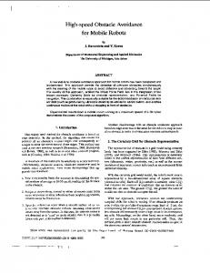
Figure 4. Block diagram of the algorithm. The raw range scan is used by the path planner to plan a path to the desired goal. Each path point contains a recommended speed dependent on the curvature of the path. The dynamic line, operating on a subset of the scan points, tries to follow the path within the acceleration limits of the robot and assures at the same time for a safe and collision free navigation. The new translational velocity v is chosen by combining the recommended speed and the acceleration constraints. The new rotational velocity ω is determined by maximizing the selection function of equation 1.
3.3 When To Replan Paths?
As a further practical issue, we also reduce the computational load of the dynamic window by choosing only a sub-
0
−0.5
−1.5 −1.5
Figure 3. An example of the distance transform and the resulting path (S means start, G goal).
Another point is the way how the path and the dynamic window work together in order to keep the robot on the path’s track and to deviate from it where shape and dynamic constraints ask for it. The dynamic window obtains path points as intermediate goal points. Thereby β 2 controls also the ‘path fidelity’. We only pass those path points which mark a change in path direction and switch to the next one if the robot is closer than a disk radius around these points. This results in a stable yet flexible driving behavior with a smoothening effect on the paths generated by the NF1.
0
−1
−2
cell with distance value
For this question we employ a quite obvious strategy. When the robot advances and senses an obstacle which goes through the planned path (thus blocking the path), the path is replanned at that position. We obtained good results with this scheme allowing to avoid all sorts of U-shaped obstacles as long as they are detectable within the local grid. Oscillating replannings in badly conditioned obstacle configurations occur occasionally but never endanger the mission to reach the goal.
Y−Coordinates [m]
Y−Coordinates [m]
0.5
1
set from the laser scan. The subset contains range readings below a certain radius. This radius is dynamic and depends on the maximum speed of the robot. A thinning strategy to remove obstacle points which are very close to each other is also used. This is especially relevant when the robot is near a wall, where many obstacle points lie close to each other. The resulting algorithm is illustrated in figure 4.
4. Distance To Collision: An Analytical Solution For Polygonal Robots Given the shape of the robot, an obstacle point O and a velocity set ( v, ω ) , this section presents a general method to determine the distance to collision as it is needed in the dynamic window approach [14][5]. To exemplify the method, a rectangular shaped robot is used. Extension to an arbitrary polygon is straight-forward although expression become more complex than equations (4)–(7). In theory, the
3052
method is not limited to polygonal shapes as long as the robot contour has an analytical expression. Instead of searching for the distance to collision in the world frame we use the robot frame { R }. This is important to note since performing the same calculations in the world frame will yield complex and intractable expressions for anything but a circular robot shape. Once this has been seen, we will need the trajectory which the obstacle point O makes in the robot frame. Then, the point P where the obstacle hits the robot can be found easily by calculating the intersection between the robot contour and the trajectory of O . No intersection means no collision with that point. The solution can be found from a simple equation system. We first introduce the vectors and variables (figure 5)
PC = P – C
particularly simple since they both have a rectangular shape. This is a further reason to use the robot coordinate system since the robot contour quite obviously always follows the axis direction of the robot frame. The left and right side of the robot can be expressed by two lines parallel to the y -axis. In the same way the front and back side can be described by two lines parallel to the x -axis. In equations (4)–(7) the collision point P = ( x c, y c ) for front, left, right and back collision is found by solving the resulting equation systems for each case: Front side: with x c ∈ [ X LEFT, X RIGHT ] 2 2 2 2 2 x c = r ± r O – Y FRONT ( xc – r ) + yc = rO ⇒ y c = Y FRONT y c = Y FRONT
Left side: with y c ∈ [ Y BACK, Y FRONT ] 2 2 2 2 2 y c = ± r O – ( X LEFT – r ) ( xc – r ) + yc = rO ⇒ x c = X LEFT x c = X LEFT
OC = O – C RC = R – C
(2)
r = C = vÚω
We determine now the circle of O as seen from the robot. This circle, dashed in figure 5, has the same center point as the circle on which the robot moves (continuous line in figure 5). Its radius, r O , is found as the length of vector O C . The equation of the circle gives 2
2
2
rO = ( x – r ) + y .
2 2 2 2 2 y c = ± r O – ( X RIGHT – r ) ( xc – r ) + yc = rO ⇒ x c = X RIGHT x c = X RIGHT
2 2 2 2 2 x c = r ± r O – Y BACK ( xc – r ) + yc = rO ⇒ y c = Y BACK y c = Y BACK
OC v
O
{R}
Y FRONT
P
P
R α C PC
Y BACK X LEFT
X RIGHT
Figure 5. The dashed circle shows the motion of an obstacle point in the robot frame { R }. The continuous circle shows the robots motion in the world frame.
C C ⋅ OC α = acos ---------------------- CC OC
(8)
d = α⋅r
(9)
A single obstacle point can collide at several positions of the robot contour. Therefore the final distance to collision, d coll , is determined as the minimum of the collision distances from all intersection points
d coll = min ( d FRONT, d LEFT, d RIGHT, d BACK ) .
RC
ω
(7)
If any of the above equation systems yields a non-imaginary solution, the robot will collide at P . The distance d travelled by the robot until collision is then calculated by
(3)
Robot position at collision
(6)
Back side: with x c ∈ [ X LEFT, X RIGHT ]
This result and the analytical expression for the robot contour gives the contour collision point P . In the case of Pygmalion and Donald (figure 7) the expressions are
O
(5)
Right side: with y c ∈ [ Y BACK, Y FRONT ]
rO = OC . All vectors are represented in the (temporarily stationary) robot coordinate system { R } which in the start point coincides the global frame, i.e. ( x, y, θ ) = ( 0, 0, 0 ) .
(4)
(10)
5. Experiments and Results Obstacle avoidance is a safety-critical task – critical for the environment, the robot and the mission. It therefore merits particular attention for the implementation on a real robot. With the real-time OS XO/2 we use [2], obstacle avoidance is implemented as a so called hard real-time tasks. The operating system schedules such a task at a given frequency while guaranteeing its completion within a specified deadline. Under full CPU load, we measure 23.2 milliseconds
3053
maximal processing time which includes dynamic line and path planning. The SICK scanners deliver new data with 10 Hz, yielding thus a cycle time of 10 Hz and the task’s deadline of 100 ms. The implementation is running on the robots Pygmalion and Donald (figure 7). 5.1 Laboratory and Simulation Experiments Identification experiments for Pygmalion yielded the values for the minimal and maximal accelerations which are needed in the dynamic window: max. translational acceler2 ation a max = 0.3m Ú s (set smaller than maximal possible for aesthetic reasons), maximal translational 2 deceleration d max = – 1.6m Ú s , maximal rotational speed ω max = ± 2.0 rad Ú s , and max. rotational acceleration 2 a ω = ± 3.3 rad Ú s . A run in simulation and in the laboratory is shown in figure 6. The figures show the superposed range readings and the trajectory of the vehicle. Several replannings were necessary to bring the vehicle to the desired positions. We also see that the rectangular robot shape is properly taken into account. A cluttered environment with outlier measurement was simulated (figure 6, top) and encountered in reality (figure 6, bottom). 5.2 Results From “Computer 2000” “Computer 2000” is an annual tradeshow for computer hard- and software at the Palais de Beaulieu exposition center in Lausanne, Switzerland. Our laboratory was present during the four days, May 2nd to May 5th 2000, Global View
2
Y−Coordinates [m]
1
0
−1
−2
−4 0
1
2 3 X−Coordinates [m]
4
5
6
4
3
y [m]
2
1
0
1
0
1
2
3
4
5
6
giving visitors the opportunity to control Pygmalion by means of its web-interface (figure 8) and to discover our institute building at EPFL. The experiment took place during normal office hours in an unmodified environment of 50 m×30 m in size which contains twelve offices, two corridors, the seminar and the mail room. Note that the environment is relatively big and implies many co-workers. This makes it impossible to prepare the environment in order to comply with the needs of a 2D laser range finder. The main concern of this experiment was to have a test-bed for our localization [1], the obstacle avoidance and the complete system as a whole. During the 28 hours of system activity, Pygmalion travelled more than 5 km and had about 60 collisions (table 1). We never observed a case where the goal was not reached due to a local minima problem. About 50 collisions were due to objects which were not visible at all to the robot’s sensors. These objects include (in decreasing frequency): (i) tables, chairs and other furniture, (ii) opened doors standing exactly in the blind zones between the two laserscanners, (iii) bags and luggage on the floor, (iv) students or staff members who play with the robot and thereby provoke collisions. We counted ten collisions of unknown origin. This because the robot ran autonomously – without constant supervision – over extended periods of time. The a posteriori reconstruction of the failure cause (by the hastily approaching operator) was very difficult in these cases. A problem which was occasionally observed was that the NF1 generated paths that cut corners in a undesirable way. Together with a low-level security rule which stops the robot if something is closer than five centimeters, this lead to situations of a blocked robot typically with doors which open into the corridor. Although no collision occurred, manual intervention was necessary.
−3
−1
Figure 7. Pygmalion and Donald. The two robots on which the algorithm has been tested. Both are non-holonomic differential drive robots sporting two SICK LMS200. They carry a VME rack with a PowerPC 604e at 300MHz and always operate in a fully autonomous mode.
7
x [m]
Figure 6. A simulation run at 1m Ús (top). A test run with the real robot in the laboratory at 0.4m Ús (bottom). In order to reach the goal in the corridor, several replannings were necessary in both experiments.
6. Conclusions and Outlook From the experiments we conclude that this approach is very practical and exhibits a well-balanced distribution of
3054
Hours of operation
28 / 4 days
Environment size
50 x 30 m
Overall travel distance
5,013 m
Maximal travel speed
0.4 m/sec
Number of missions
724
Number of localization cycles
145,433
Number of localization lost-situation
0
Number of unknown collisions
~ 10
Table 1. Overall statistics of the “Computer 2000” event.
Future work will address the problem of highly dynamic obstacles and an improved local path planning. The results, particularly from the “Computer 2000” event, are also a compelling demand for 3D sensing. Even in this structured environment, the most significant failure cause was the 2Dassumption respectively its violation. If service or personal robots shall be successful in applications whose environments can not be controlled, 3D sensing will be mandatory.
References [1]
the computational load to the model and the planning stage. Shape and dynamics is taken into account by a reduced, fast dynamic window and the local minima problem is significantly diminished by a path planner operating on a local grid. The use of a simple curvature-dependent velocity profile along the path allows to reduce the dynamic window to a dynamic line. This makes the approach fast even for polygonal robots. The analytical solution of the distance to collision we presented allows further an on-the-fly changing robot contour – for example from the presence or absence of a payload. This would be difficult with hard-coded look-up tables or a simplified robot shape. Clearly, The NF1 path planner is a suboptimal choice. It has the already mentioned property to generate paths that cut corners and produces in general an unsmooth robot motion. Improvements exist and we recommend to use them although the NF1 seduces by its simplicity. A more sophisticated path planner would eventually reduce the maximal achievable cycle time.
[2]
[3]
[4]
[5]
[6] [7]
[8]
[9]
[10] [11]
[12]
[13]
[14]
Figure 8. The Pygmalion web-interface. It provides context-sensitive menus with intuitive click-and-move-there commands for robot teleoperation. Four different realtime streams constitute the visual feedback: an external web-cam (top-right), an on-board camera (top middle), raw data from the laser range finder (top-left) and the robot animated in its model map (left middle). By clicking onto the map an office is defined as destination, clicking onto the camera image turns the robot and clicking on the laser scanner image defines a local ( x, y ) -goal.
[15]
[16]
[17]
3055
Arras K.O., Tomatis N., Jensen B., Siegwart R., “Multisensor On-the-Fly Localization: Precision and Reliability for Applications”, Robotics and Autonomous Systems, 34 (2-3), p.131143, 2001. Brega R., Tomatis N., Arras K.O., "The Need for Autonomy and Real-Time in Mobile Robotics: A Case Study of XO/2 and Pygmalion," IEEE/RSJ Int. Conference on Intelligent Robots and Systems, Takamatsu, Japan, 2000. See also www.xo2.org Brock O., Khatib O., "High-Speed Navigation Using the Global Dynamic Window Approach," IEEE Int. Conference on Robotics and Automation, Detroit, USA, 1999. Feder H.J.S., Slotin J.J.E., "Real-Time Path Planning Using Harmonic Potentials in Dynamic Environments," IEEE Int. Conf. on Robotics and Automation, Albuquerque, USA, 1997. Fox D., Burgard W., Thrun S., "The Dynamic Window Approach to Collision Avoidance," IEEE Robotics and Automation Magazine, 4(1), pp. 23-33, March 1997. Khatib O., "Real-Time Obstacle Avoidance for Manipulators and Mobile Robots," Int. J. of Robotics Research, 5(1), 1986. Khatib M., Jaouni H., Chatila R., Laumod J.P., "Dynamic Path Modification for Car-Like Nonholonomic Mobile Robots," IEEE Int. Conf. on Robotics and Automation, Albuquerque, USA, 1997. Khatib M., Chatila R., "An Extended Potential Field Approach for Mobile Robot Sensor-Based Motion," Intelligent Autonomous Systems (IAS-4), IOS Press, 1995. Koren Y., Borenstein J., “Potential Field Methods and Their Inherent Limitations for Mobile Robot Navigation,” IEEE Int. Conf. on Robotics and Automation, Sacramento, USA, 1991. Latombe J.-C., Robot motion planning, Kluwer, 1991. Minguez J., Montano L., “Nearness Diagram Navigation (ND): A New Real Time Collision Avoidance Approach, IEEE/RSJ Int. Conf. on Intelligent Robots and Systems, Takamatsu, 2000. Quinlan S., Khatib O., "Elastic Bands: Connecting Path Planning and Control," IEEE Int. Conf. on Robotics and Automation, Atlanta, USA, 1993. Schlegel C., "Fast Local Obstacle Avoidance Under Kinematic and Dynamic Constraints," IEEE/RSJ Int. Conf. on Intelligent Robots and Systems, Victoria B.C., Canada, 1998. Simmons R., "The Curvature Velocity Method for Local Obstacle Avoidance," IEEE Int. Conf. on Robotics and Automation, Minneapolis, USA, 1996. Simmons R., Nak Young Ko, "The Lane-Curvature Method for Local Obstacle Avoidance," IEEE/RSJ Int. Conference on Intelligent Robots and Systems, Victoria B.C., Canada, 1998. Ulrich I., Borenstein J. "VFH+: Reliable Obstacle Avoidance for Fast Mobile Robots," IEEE Int. Conference on Robotics and Automation, Leuven, Belgium, 1998. Ulrich I., Borenstein J. "VFH*: Local Obstacle Avoidance with Look-Ahead Verification," IEEE Int. Conference on Robotics and Automation, San Francisco, USA, 2000.