Jul 31, 2015 - n = âlog2(N)â-bit number requires a minimum of n qubits in the computational register (to store the re-. arXiv:1507.08852v1 [quant-ph] 31 Jul ...
Realization of a scalable Shor algorithm T. Monz,1 D. Nigg,1 E. A. Martinez,1 M. F. Brandl,1 P. Schindler,1 R. Rines,2 S. X. Wang,2 I. L. Chuang,2 and R. Blatt1, 3
arXiv:1507.08852v1 [quant-ph] 31 Jul 2015
2
1 Institut f¨ ur Experimentalphysik, Universit¨ at Innsbruck, Technikerstr. 25, A-6020 Innsbruck, Austria Center for Ultracold Atoms, Massachusetts Institute of Technology, 77 Massachusetts Ave, Cambridge, MA, USA 3 Institut f¨ ur Quantenoptik und Quanteninformation, ¨ Osterreichische Akademie der Wissenschaften, Otto-Hittmair-Platz 1, A-6020 Innsbruck, Austria (Dated: August 3, 2015)
Quantum computers are able to outperform classical algorithms. This was long recognized by the visionary Richard Feynman who pointed out in the 1980s that quantum mechanical problems were better solved with quantum machines. It was only in 1994 that Peter Shor came up with an algorithm that is able to calculate the prime factors of a large number vastly more efficiently than known possible with a classical computer [1]. This paradigmatic algorithm stimulated the flourishing research in quantum information processing and the quest for an actual implementation of a quantum computer. Over the last fifteen years, using skillful optimizations, several instances of a Shor algorithm have been implemented on various platforms and clearly proved the feasibility of quantum factoring [2–7]. For general scalability, though, a different approach has to be pursued [8]. Here, we report the realization of a fully scalable Shor algorithm as proposed by Kitaev [9]. For this, we demonstrate factoring the number fifteen by effectively employing and controlling seven qubits and four “cache-qubits”, together with the implementation of generalized arithmetic operations, known as modular multipliers. The scalable algorithm has been realized with an ion-trap quantum computer exhibiting success probabilities in excess of 90%. PACS numbers: 03.67.Lx, 37.10.Ty, 32.80.Qk
Shor’s algorithm for factoring integers [1] is one of the examples where a quantum computer (QC) outperforms the most efficient known classical algorithms. Experimentally, its implementation is highly demanding as it requires both a sufficiently large quantum register and high-fidelity control. Clearly, such challenging requirements raise the question whether optimizations and experimental shortcuts are possible. While optimizations, especially system-specific or architectural, certainly are possible, for a demonstration of Shor’s algorithm to be scalable special care has to be taken not to oversimplify the implementation - for instance by employing knowledge about the solution prior to the actual experimental implementation - as pointed out in Ref. 8. In order to elucidate the general task at hand, we first explain and exemplify Shor’s algorithm for factoring the number 15 in a (quantum) circuit model. Subsequently, we show how this circuit model is translated for and implemented with an ion-trap quantum computer. How does Shor’s algorithm work? Here is a classical recipe to find the factors of a large number. As an example, assume the number we want to factor is N = 15. Then pick a random number a ∈ [2, N − 1] (which we call the base in the following), say a = 7. Check if the greatest common divisor gcd(a, N ) = 1, otherwise a factor is already determined. This is the case for a = {3, 5, 6, 9, 10, 12}. Next, calculate the modular exponentiations ax mod N for x = 0, 1, 2... and find its period r: the first x > 0 such that ax mod N = 1. Given the period r, finding the factors requires calculating the greatest common divisors of ar/2 ± 1 and N ,
which is classically efficiently possible - for instance using Euclid’s algorithm. For our example (N = 15, a = 7) the modular exponentiation yields 1, 7, 4, 13, 1, ..., which has period 4. The greatest common divisor of ar/2 ± 1 = 74/2 ± 1 = {48, 50} and N = 15 are {3, 5}, the non-trivial factors of N . For the chosen example N = 15, the cases a = {4, 11, 14} have periodicity r = 2 and would only require a single multiplication step (a2 mod N = 1), which is considered an “easy” case [8]. Note that the periodicity for a chosen a can not be predicted. How can this recipe be implemented in a QC? A QC also has to calculate ax mod N in a computational register for x = 0, 1, 2... and then extract r. However, using the quantum Fourier-transform (QFT), this can be done with high probability in a single step (compared to r steps classically). Here, x is stored in a quantum register consisting of k qubits, or period-register, which is in a superposition of 0 to 2k − 1. The superposition in the period-register on its own does not provide a speedup compared to a classical computer. Measuring the periodregister would collapse the state and only return a single value, say x1 , and the corresponding answer to ax1 mod N in the computational register. However, if the QFT is applied to the period-register, the period of ax mod N can be extracted from O(1) measurements. What are the requirements and challenges to implement Shor’s algorithm? First, we focus on the periodregister, to subsequently address modular exponentiation in the computational register. Factoring N , an n = dlog2 (N )e-bit number requires a minimum of n qubits in the computational register (to store the re-
2 H
H
H
90
H
H
90
45
H
H
H
H
90
H
H
90
45
H
H
H
H
90
H
H
90
45
H
FIG. 1: Circuit diagram of Shor’s algorithm for factoring 15 based on Kitaev’s approach for: a) a generic base a; and the specific circuit representations for the modular multipliers; b) The actual implementation for factoring 15 to base 11, optimised for the single input state it is subject to; c) Kitaev’s approach to Shor’s algorithm for the bases {2,7,8,13}: the optimised map of the first multiplier is identical in all 4 cases, the last multiplier is implemented with full modular multipliers as depicted in d); d) Circuit diagrams of the modular multipliers of the form a mod N for bases a={2,7,8,11,13}.
sults of ax mod N ) and generally about 2n qubits in the period-register [10]. Thus even a seemingly simple example such as factoring 15 (an n = 4 -bit number), would require 3n = 12 qubits when implemented in this straightforward way. These qubits then would have to be manipulated with high fidelity gates. Given the current state-of-the-art control over quantum systems [11], such an approach likely yields an unsatisfying performance. However, a full quantum implementation of this part of the algorithm is not really necessary. In Ref. 9 Kitaev notes that, if only the classical information of the QFT (such as the period r) is of interest, 2n qubits subject to a QFT can be replaced by a single qubit. This approach, however, requires qubit-recycling (specifically: in-sequence single-qubit readout and state reinitialization) paired with feed-forward to compensate for the reduced system size. In the following, Kitaev’s QFT will be referred to as KQFT(M ) . It replaces a QFT acting on M qubits with a semiclassical QFT acting repeatedly on a single qubit. Similar applications of Kitaev’s approach to a semiclassical QFT in quantum algorithms have been investigated in Refs. [12–14]. For the implementation of Shor’s algorithm, Kitaev’s approach provides a reduction from the previous n computational qubits and 2n QFT qubits (in total 3n qubits) to only n computational-qubits and 1 KQFT(2n) qubit (in total n + 1 qubits). A notably more challenging aspect than the QFT, and the second key-ingredient of Shor’s algorithm, is the mod-
ular exponentiation, which admits these general simplifications: (i) Considering Kitaev’s approach (see Fig. 1), the input state |1i (in decimal representation) is subject to a conditional multiplication based on the most-significant bit k of the period register. At most there will be two results after this first step. It follows that, for the very first step it is sufficient to implement an optimized operk ation that conditionally maps |1i → |a2 mod N i. Considering the importance of a high-fidelity multiplication (with its performance being fed-forward to all subsequent qubits), this efficient simplification improves the overall performance of experimental realizations. (ii) Subsequent multipliers can similarly be replaced with maps by considering only possible outputs of the previous multiplications. However, using such maps will become exponentially more challenging, as the number of input and output states to be considered grows exponentially with the number of steps: after n steps, 2n > N possible outcomes need to be considered - a numerical task as challenging as factoring N by classical means. Thus, controlled full modular multipliers need to be implemented. Fig. 2 shows the experimentally obtained truth table for the modular multiplier (2 mod 15) (see also supplementary material for modular multipliers with bases {7, 8, 11, 13}). These quantum circuits can be efficiently derived from classical procedures using a variety of standard techniques for reversible quantum arithmetic and local logic optimization [15, 16].
3
a)
b)
0.7
0.7
0.6
0.6
0.5
0.5
0.4
0.4
0.3
0.3
0.2
0.2
0.1
0.1
0
0 0
1
2
0 3
4
5
6
Input
7
8
9 10 11 12 13 14 15
0
1
2
3
4
5
6
7
8
9
15 14 13 12 11 10
1
2
3
4
5
6
7
Input
Output
8
9 10 11 12 13 14 15
0
1
2
3
4
5
6
7
8
9
15 14 13 12 11 10
Output
FIG. 2: Experimentally obtained truth table of the controlled 2 modular 15 multiplier: a) with the control-qubit being in state 0, the truth table corresponds to the identity operation; b) when the control qubit triggers the multiplication, the truth table illustrates the multiplication of the input state with 2 modular 15.
(iii) The very last multiplier allows one more simplification: Considering that the actual results of the modular exponentiation are not required for Shor’s algorithm (as only the period encoded in the period-register is of interest), the last multiplier only has to create the correct amount of correlations between the period register and the computation register. Local operations after the conditional (entangling) operations may be discarded to facilitate the final multiplication without affecting the results of the implementation. (iv) In rare cases, certain qubits are not subject to operations in the computation. Thus, these qubits can be removed from the algorithm entirely. For larger scale quantum computation, optimization steps (i), (iii) and (iv) will only marginally effect the performance of the implementation. They represent only a small subset of the entire computation which mainly consists of the full modular multipliers. Thus, the realization of these modular multipliers is a core requirement for scalable implementations of Shor’s algorithm. Furthermore, Kitaev’s approach requires in-sequence measurements, qubit-recycling to reset the measured qubit, feed-forward of gate settings based on previous measurement results, as well as numerous controlled quantum operations - tasks that have not been realized in a combined experiment so far. We demonstrate these techniques in our realization of Shor’s algorithm in an ion-trap quantum computer, with five 40 Ca+ ions in a linear Paul trap. The qubit is encoded in the ground state S1/2 (m = −1/2) = |1i and the metastable state D5/2 (m = −1/2) = |0i. The universal set of quantum gates consists of the entan-
gling Mølmer-Sørenson interaction [17], collective opP (i) erations of the form exp(−i θ2 Sφ ) with Sφ = i σφ , (i)
(i)
(i)
(i)
σφ = cos(φ)σx + sin(φ)σy , σ{x,y} the Pauli operators of qubit i, θ = Ωt determined by the Rabi frequency Ω and laser pulse duration t, φ determined by the relative phase between qubit and laser, and single qubit phase rotations induced by localized AC-Stark shifts (for more details see the supplementary material and Ref. 18). Unitary operations illustrated in Fig. 1 are decomposed into primitive components such as two-target C-NOT and CSWAP gates (or gates with global symmetries such as the four-target C-NOT employed here), from which an adaptation of the GRAPE algorithm [19] can efficiently derive an equivalent sequence of laser pulses acting on only the relevant qubits. The problem with this approach is that the resulting sequence generally includes operations acting on all qubits. Implementing the optimized 3-qubit operations on a 5-ion string therefore requires decoupling of the remaining qubits from the computation space. We spectroscopically decouple qubits by transferring any information from |Si → |D0 i = D5/2 (m = −5/2) and |Di → |S 0 i = S1/2 (m = 1/2). Here, the subspace {|S 0 i, |D0 i} serves as a readily available “quantum cache” to store and retrieve quantum information in order to facilitate quantum computations. Finally, to complete the toolbox necessary for a Kitaev’s approach to Shor’s algorithm, we also implement single qubit readout (by encoding all other qubits in the {|Di, |D0 i} subspace and subsequent electron shelving [20] on the S1/2 ↔ P1/2 transition), feed-forward (by storing counts detected during the single-qubit read-
4 1.2
Shor: 15 base 2 SSO = 0.97
Shor: 15 base 7 SSO = 0.96
Shor: 15 base 8 SSO = 0.97
Shor: 15 base 11 Shor: 15 base 13 SSO = 0.90 SSO = 0.97
0 1 2 3 4 5 6 7
0 1 2 3 4 5 6 7 QFT output state
0 1 2 3 4 5 6 7
1.0
Output state rel. probability
out [21] in a classical register and subsequent conditional laser pulses) and state-reinitialization (using optical pumping for the ion, and Raman-cooling [22, 23] for the motional state of the ion string). The pulse sequences and additional information on the implementation on the modular multipliers are available as supplementary material. The key differences of our implementation with respect to previous realizations of Shor’s algorithm are: a) the entire quantum register is employed, without sparing qubits that don’t partake in the calculation; b) besides the trivial first multiplication step (corresponding to r = 2 for a = {4, 11, 14}, realized only once for a = 11), all nontrivial modular multipliers a = {2, 7, 8, 13} have been realized and applied; and c) Kitaev’s originally proposed scheme is implemented with complete qubit recycling – doing both readout and reinitialization on the very same physical qubit. This is especially important for factoring 15 with base {2,7,8,13}, as at least two steps are required for the semiclassical QFT. In our realization we go beyond the minimal implementation of Shor’s algorithm and not only employ all 7 qubits (comprised of 4 physical qubits in the computational register, 1 qubit in the periodicity register - recycled twice, plus additional cache qubits), but also include multiplication with up to the fourth power (although they correspond to the identity operation). This represents a realistic attempt at a scalable implementation of Shor’s algorithm as the entire qubit register remains subject to decoherence processes along the computation, and no simplifications are employed which presume prior knowledge of the solution. The measurement results for base a = {2, 7, 8, 11, 13} with periodicities r = {4, 4, 4, 2, 4} are shown in Fig. 3. In order to quantify the performance of the implementation, previous realizations mainly focused on the squared statistical overlap (SSO) [24], the classical equivalent to the Uhlmann fidelity [10]. While we achieved an SSO of {0.968(1), 0.964(1), 0.966(1), 0.901(1), 0.972(1)} for the case of a={2,7,8,11,13}, we argue that this does not answer the question of a user in front of the quantum computer: “What is the periodicity?” Shor’s algorithm allows one to deduce the periodicity with high probability from a single-shot measurement, since the output of the QFT is, in the exact case, a ratio of integers, where the denominator gives the desired periodicity. This periodicity is extracted using a continued fraction expansion, applied to x/2k , a good approximation of the ideal case when k, the number of qubits, is sufficiently large. For the realised examples, the probabilistic nature of Shor’s algorithm becomes clear: the output state 0 never yields any information. For periodicity 4 (and 3 qubits in the period-register), the output state 4 suggests a fraction 1 4 23 = 2 , thus a periodicity of 2 and also fails. For peridocity 4, only the output states 2 and 6 allow one to deduce the correct periodicity. In our realisations to bases a = {2, 7, 8, 11, 13}, the probabilities to obtain output
0.8
0.6
0.4
0.2
0.0 0 1 2 3 4 5 6 7
0 1 2 3 4 5 6 7
FIG. 3: Results and correct order-assign probability for the different implementations to factor 15: a) 3-digit results (in decimal representation) of Shor’s algorithm for the different bases. The ideal data (red) for periodicity {2, 4} is superimposed on the raw data (blue). The squared statistical overlap is larger than 90% for all cases.
states that allow the derivation of the correct periodicity are {56(2), 51(2), 54(2), 47(2), 50(2)}%. Thus, a confidence that the correct periodicity is obtained at a level of more than 99%, requires the experiment to run about 8 times. In summary, we have presented the realization of Kitaev’s vision to realize a scalable Shor’s algorithm with 3-digit resolution to factor 15 using bases {2,7,8,11,13}. Here, a semiclassical QFT combined with single-qubit readout, feed-forward and qubit recycling was successfully employed. Compared to the traditional algorithm, the required number of qubits can thus be reduced by almost a factor of 3. Furthermore, the entire quantum register has been subject to the computation in a “blackbox” fashion. Employing the equivalent of a quantum cache by spectroscopic decoupling significantly facilitated the derivation of the necessary pulse sequences to achieve high-fidelity results. In the future, spectroscopic decoupling might be replaced by physically moving the qubits from the computational zone using segmented traps [25]. Our investigations also reveal some open questions and problems for current and upcoming realizations of Shor’s algorithm, which also apply to several other largescale quantum algorithms of interest: particularily, finding system-specific implementations of suitable pulse sequences to realize the desired evolution. The presented operations were efficiently constructed from classical circuits, and decomposed into manageable unitary building blocks (quantum gates) for which pulse sequences were obtained by an adapted GRAPE algorithm. Thus, the presented successful implementation in an ion-trap quantum computer demonstrates a viable approach to a scalable Shor algorithm. We gratefully acknowledge support by the Austrian Science Fund (FWF), through the SFB FoQus (FWF Project No. F4002-N16), by the European Commission (AQUTE), the NSF iQuISE IGERT, as well as the Institut f¨ ur Quantenoptik und Quanteninformation GmbH.
5 EM is a recipient of a DOC Fellowship of the Austrian Academy of Sciences. This research was funded by the Office of the Director of National Intelligence (ODNI), Intelligence Advanced Research Projects Activity (IARPA), through the Army Research Office grant W911NF-10-1-0284. All statements of fact, opinion or conclusions contained herein are those of the authors and should not be construed as representing the official views or policies of IARPA, the ODNI, or the U.S. Government.
[1] P. W. Shor, Foundations of Computer Science, 1994 Proceedings., 35th Annual Symposium on pp. 124–134 (1994). [2] A. Politi, J. C. F. Matthews, and J. L. O’Brien, Science 325, 1221 (2009). [3] E. Martin-Lopez, A. Laing, T. Lawson, R. Alvarez, X.-Q. Zhou, and J. L. O’Brien, Nat Photon advance online publication (2012). [4] E. Lucero, R. Barends, Y. Chen, J. Kelly, M. Mariantoni, A. Megrant, P. O/’Malley, D. Sank, A. Vainsencher, J. Wenner, et al., Nat Phys 8, 719 (2012). [5] C. Y. Lu, D. E. Browne, T. Yang, and J. W. Pan, Physical Review Letters 99, 250504+ (2007). [6] B. P. Lanyon, T. J. Weinhold, N. K. Langford, M. Barbieri, D. F. V. James, A. Gilchrist, and A. G. White, Physical Review Letters 99, 250505+ (2007). [7] L. M. K. Vandersypen, M. Steffen, G. Breyta, C. S. Yannoni, M. H. Sherwood, and I. L. Chuang, Nature 414, 883 (2001). [8] J. A. Smolin, G. Smith, and A. Vargo, Pretending to factor large numbers on a quantum computer (2013), 1301.7007, URL http://arxiv.org/abs/1301.7007. [9] Kitaev (1995), quant-ph/9511026. [10] M. A. Nielsen and I. L. Chuang, Quantum Computation and Quantum Information (Cambridge Series on Information and the Natural Sciences) (Cambridge University Press, 2004), 1st ed., ISBN 0521635039. [11] K. Southwell, Quantum Coherence (Nature Insight), Nature 453, 1003 (2008). [12] R. B. Griffiths and C. S. Niu, Physical Review Letters 76, 3228 (1996). [13] S. Parker and M. B. Plenio, Physical Review Letters 85, 3049 (2000). [14] M. Mosca and A. Ekert, in Quantum Computing and Quantum Communications, edited by C. Williams (Springer Berlin Heidelberg, 1999), vol. 1509 of Lecture Notes in Computer Science, pp. 174–188. [15] V. Vedral, A. Barenco, and A. Ekert, Physical Review A 54, 147 (1996), ISSN 1050-2947, URL http://dx.doi. org/10.1103/physreva.54.147. [16] R. Van Meter and K. M. Itoh, Physical Review A 71 (2005), ISSN 1050-2947, URL http://dx.doi.org/10. 1103/physreva.71.052320. [17] A. Sørensen and K. Mølmer, Phys. Rev. Lett. 82, 1971 (1999), quant-ph/9810039. [18] P. Schindler, D. Nigg, T. Monz, J. T. Barreiro, E. Martinez, S. X. Wang, S. Quint, M. F. Brandl, V. Nebendahl, C. F. Roos, et al., New Journal of Physics 15, 123012+ (2013), ISSN 1367-2630, URL http://dx.doi.org/10.
1088/1367-2630/15/12/123012. [19] V. Nebendahl, H. H¨ affner, and C. F. Roos, Phys. Rev. A 79, 012312 (2009). [20] H. Dehmelt, Bull. Am. Phys. Soc. 20, 60 (1975). [21] M. Riebe, H. Haffner, C. F. Roos, W. Hansel, J. Benhelm, G. P. T. Lancaster, T. W. Korber, C. Becher, F. SchmidtKaler, D. F. V. James, et al., Nature 429, 734 (2004). [22] D. J. Wineland, C. Monroe, W. M. Itano, D. Leibfried, B. E. King, and D. M. Meekhof, Journal of Research of the National Institute of Standards and Technology 103, 259 (1997), quant-ph/9710025, URL http://arxiv.org/ abs/quant-ph/9710025. [23] I. Marzoli, J. Cirac, R. Blatt, and P. Zoller, Physical Review A 49, 2771 (1994), ISSN 1050-2947, URL http: //dx.doi.org/10.1103/physreva.49.2771. [24] J. Chiaverini, J. Britton, D. Leibfried, E. Knill, M. D. Barrett, R. B. Blakestad, W. M. Itano, J. D. Jost, C. Langer, R. Ozeri, et al., Science 308, 997 (2005), ISSN 1095-9203, URL http://dx.doi.org/10.1126/science. 1110335. [25] D. Kielpinski, C. Monroe, and D. J. Wineland, Nature 417, 709 (2002). [26] V. Nebendahl, Master’s thesis, University of Innsbruck, Austria (2008), URL http://heart-c704.uibk.ac.at/ publications/diploma/diplom_nebendahl.pdf.
6 Supplementary Material Pulse sequences
In the following, the pulse sequences employed in the experiment are discussed in more detail. The nomenclature is as follows: The collective operations on the S1/2 (m = −1/2) ↔ D5/2 (m = −1/2) transitions, addressing all ion-qubits, realize the unitary operation
D-state manifold. Here, the quantum information is protected against shelving light on the S1/2 ↔ P1/2 transition - the ion will not scatter any photons. Using light resonant with the S1/2 (m = −1/2) ↔ D5/2 (m = −5/2) transition (denoted by R2 (θ, φ)), a refocusing sequence of the form R2 (0.5, 0) · Sz (1, i) · R2 (0.5, 0) efficiently encodes all but qubit i in D5/2 (m = −1/2) and D5/2 (m = −5/2). Subsequently, the entire quantum register may be subject to shelving light, yet only qubit i will be projected.
π R(θ, φ) = exp(−i θSφ ) 2 with the collective spin operator X (i) X Sφ = σφ = cos(φπ)σx(i) + sin(φπ)σy(i) i
i (i)
based on the Pauli operators σ{x,y,z} acting on qubit qubit i. Here, the rotation angle θ is defined by θ = Ωt π with the Rabi frequency Ω and the laser pulse duration t. In this notation, a bit flip around σx corresponds to R(1, 0). The collective operations are supplemented by single-qubit phase shifts of the form Sz (θ, i) = exp(−i
θπ (i) σ ). 2 z
The phase shift is realized by illuminating a single qubit with a tightly focused laser beam detuned −20 MHz from the carrier transition. Here, the induced AC-Stark shift ∆AC implements the desired phase shift, with the rotat tion angle θ = ∆AC depending on the pulse duration π t. In combination, collective operations and single-qubit phase shifts allow us to implement arbitrary local operations. A universal set of quantum gates, capable of implementing any desired unitary operation, can be realized by combining these arbitrary local operations with an entangling interaction. In our experiment, we employ the Mølmer-Sørensen (MS) interaction [17] to realize entangling operations of the form
In-sequence detection and feed-forward
When all qubits that need to be protected against projection have been encoded in the {D5/2 (m = −1/2), D5/2 (m = −5/2)} manifold, light at 397 nm resonant with the S1/2 ↔ P1/2 transition state-dependently scatters photons an the remaining ion-qubits. The illumination time is set to 300 µs. A histogram of the photon counts detected at the photomultiplier tube is shown in Fig. 4. Using counter electronics with discriminator set at 4 counts within the detection window, the state D with a mean count rate of 0.24 counts/ms (or 0.07 counts within the detection window) and state S with a mean countrate of 48 counts/ms (or 14.4 counts in the detection window) can be distinguished with a confidence better than 99.8%. The boolean output of the discriminator is subsequently used in the electronics for state-dependent pulses and thus state-dependent operations.
π M S(θ) = exp(−i θSx2 ) 4 P (i) with Sx = σx . Using this notation, the maximally entangling M S( 12 ) operation applied onto the N -qubit state |0 . . . 0i directly creates the N -qubit GHZ state.
Single-qubit measurement
Electron-shelving [20] on the S1/2 ↔ P1/2 transition addresses, and thus projects, all qubits of the quantum register. For Kitaev’s implementation, however, only one qubit needs to be measured. With collective illumination, this can be achieved by transfering quantum information encoded in qubits that should not be measured into the
FIG. 4: In-sequence photon-count histogram: Using a detection window of 300 µs, the photomultiplier tube collects on average 0.07 counts when the qubit is in state D and 14.4 counts when it is in state S. As can be seen in the figure, these two Poisson distributions are well distinguishable.
7 Recooling and Qubit-reset
Scattering photons during the detection window heats the ion-string and can lower the quality of subsequent quantum operations applied to the register. Therefore recooling of the ion-string after the illumination with electron-shelving light is necessary. However, this recooling must not destroy any quantum information stored in the other qubits. Considering that the hidden quantum information is stored in the D5/2 manifold, we employ 3-beam Raman-cooling [22, 23] in the S1/2 ↔ P1/2 manifold. The Raman light field, consisting of σ + and π light with respect to the quantization axis, is detuned by 1.5 GHz from the resonant S1/2 ↔ P1/2 transition. The relative detuning between σ + and π is chosen such that it creates resonant coupling between S1/2 (m = −1/2) ⊗ |ni ↔ S1/2 (m = 1/2) ⊗ |n − 1i, with |ni representing the quantized axial state of motion of the ion. The transfer is reset by resonant σ − light. Raman cooling is employed for 500 µs. The qubit is reinitialized after cooling by an additional 50 µs of σ − light. However, if the measured qubit was found to be in state D, neither does the measurement heat the ion string nor does the Raman cooling affect the register. Therefore the qubit is transferred from D5/2 (m = −1/2) to S1/2 (m = 1/2) (which was depleted by the previous 50 µs of σ − ). An additional pulse of σ − light for 50 µs finally initializes the qubit, regardless whether it was projected into S or D. During the entire time when the qubit is subject to Raman cooling or initializing σ − light, a repump laser at 866 nm is applied to prevent population trapping in the D3/2 manifold due to spontaneous decay from the P1/2 state to D3/2 . Pulse sequence optimisation
For a sufficiently large Hilbert-space it will no longer be possible to directly optimize unitary operations acting on the entire register. Decomposing the necessary unitary operations into building blocks acting on smaller register sizes will allow one the use of optimized pulse sequences for large-scale quantum computation. From a methodological point of view it may be preferred to physically decouple the qubits from any interactions (for instance by splitting and moving part of ion-qubit quantum register out of an interaction region, such as proposed in Ref. 25). However, given the technical requirements and challenges for splitting and moving ionstrings, we focus on spectroscopically decoupling certain ion-qubits from the interaction. In particular, we spectroscopically decouple an ion from subsequent interaction by transferring any quantum information from the {S1/2 (m = −1/2), D5/2 (m = −1/2)} manifold to the {S1/2 (m = 1/2), D5/2 (m = −5/2)} manifold using refocusing techniques on the D5/2 (m = −1/2) ↔ S1/2 (m =
1/2) and S1/2 (m = −1/2) ↔ D5/2 (m = −5/2) transitions. Using this approach, we optimise the controlled swap operation in a 3-qubit Hilbert space rather than a 5-qubit Hilbert space.
Controlled-SWAP
The controlled-SWAP operation, also known as Fredkin operation, plays a crucial role in the modular multiplication. For its implementation, however, we could not derive a pulse sequence that can incorporate an arbitrary number of spectator qubits — qubits, that should be subject to the identity operation — in the presented case, i.e. 2 spectator qubits in the computational register. However, using decoupling of spectator qubits, this additional requirement on the implementation is not necessary. Using pulse sequence optimization [19], we obtained a sequence for the exact three-qubit case as shown in Tab. I. In total the sequence consists of 18 pulses, including 4 MS interactions. Pulse Nr. Pulse Pulse Nr. 1 R(1/2, 1/2) 10 2 Sz (3/2, 3) 11 3 M S(4/8) 12 4 Sz (3/2, 2) 13 5 Sz (1/2, 3) 14 6 R(3/4, 0) 15 7 M S(6/8) 16 8 Sz (3/2, 2) 17 9 M S(4/8) 18
Pulse R(1/2, 1) Sz (1/4, 2) Sz (3/2, 3) M S(4/8) Sz (3/2, 2) Sz (3/2, 1) R(1/2, 1) Sz (3/2, 1) Sz (3/2, 2)
TABLE I: Controlled SWAP operation: In a system of three ion-qubits, qubit 1 represents the control qubit and qubits {2, 3} are to be swapped depending on the state of the first qubit. Note that this sequence only works for three-qubit systems. Spectator qubits would not experience the identity operation.
Four-Target Controlled-NOT
The modular multipliers (7 mod 15) and (13 mod 15) require, besides Fredkin operations, also CNOT operations acting on all qubits in the computational register. Such an operation can be implemented (see Ref. 26 (p.90, eq. 5.21) ) with 2 MS operations plus local operations only - regardless of the size of the computational register. The respective sequence is shown in Tab. II.
8 Pulse Nr. Pulse Pulse Nr. Pulse 1 R(1/2, 1) 6 M S(1/4) 2 Sz (3/2, 1) 7 R(3/4, 0) 3 M S(3/4) 8 Sz (3/2, 1) 4 R(5/4, 1) 9 R(1/2, 0) 5 Sz (1, 1) TABLE II: Four-target controlled NOT: Depending on the state of qubit one, the remaining four qubits {2-5} are subject to a conditional NOT operation.
Two-Target Controlled-NOT
There exists an analytic solution to realize multi-target controlled-NOT operations in the presence of spectator qubits with the presented set of gates [26] - as required for the {2, 7, 8, 13}2 mod 15 multiplier. However, we find that performing decoupling of subsets of qubits of the quantum register prior to the application of the multitarget controlled-NOT operation presented above both facilitates the optimisation, and improves the performance of the realisation of a two-target controlled-NOT operation. Thus, the required two-target controlled-NOT operation is implemented via (i) decoupling qubits 2 and 4, (ii) performing a multi-target controlled-not on all qubits with the first qubit acting as control, and (iii) recoupling of qubits 2 and 4.
Controlled Quantum Modular Multipliers
Based on the decomposition shown in Fig. 1d) and the respective pulse sequences outlined in the previous section, we investigate the performance of the building blocks as well as the respective conditional multipliers. In the following, the fidelities are defined as mean probabilities and standard deviations to observe the correct output state. The elements in the respective truth tables have been obtained as average over 200 repetitions. • The Fredkin operation, controlled by qubit 1 and acting on qubits {35, 23, 34, 45}, yields fidelities of {76(4), 73(6), 72(4), 68(7)}%. These numbers are consistent with MS gate interactions at a fidelity of about 95% acting on three ions (in the presence of two decoupled ions) and local operations at a fidelity of 99.3%. • The 4-target CNOT gate operates at a fidelity of 86(3)%. • Considering the quality for modular multipliers of ({2, 4, 7, 8, 11, 13} mod 15), we find fidelities of {48(5), 40(5), 50(6), 46(5), 38(5)}%. This performance is consistent with the multiplication of the performance of the individual building blocks: {37(6), 36(5), 37(6), 48(5), 36(5)}%.
9
FIG. 5: Controlled modular multipliers: While the full truth tables have been obtained, for improved visibility only the subset of data for the computational register (in decimal basis) is presented for modular multipliers ({2, 7, 8, 11, 13} mod 15) where the control bit maps from |0i to |0i (a,c,e,g,i) as well as when |1i maps onto |1i (b,d,f,h,j). When the control qubit is in state |0i, one expects to find the identity operation implemented, as shown in (a,c,e,g,i). If the control qubit is in state |1i, the input state gets multiplied by ({2, 7, 8, 11, 13}) mod 15. This behaviour is visually demonstrated as the output state increases in steps of {2, 7, 8, 11, 13} until it reaches 15, where the output is then returned to its value modulo 15.