School of Education Technology. Jadavpur University, Kolkata. ABSTRACT. This paper addresses the problem of recognizing semantic content from images and ...
International Journal of Computer Applications (0975 – 8887) Volume 73– No.15, July 2013
Recognition of Semantic Content in Image and Video Punam R. Karmokar
Ranjan Parekh
School of Education Technology, Jadavpur University, Kolkata
School of Education Technology Jadavpur University, Kolkata
ABSTRACT This paper addresses the problem of recognizing semantic content from images and video for content based retrieval purposes. Semantic features are derived from a collection of low-level features based on color, texture and shape combined together to form composite feature vectors. Both Manhattan distance and Neural Networks are used as classifiers for recognition purposes. Discrimination is done using five semantic classes viz. mountains, forests, flowers, highways and buildings. The composite feature is represented by a 26-element vector comprising of 18 color components, 2 texture components and 6 shape components.
General Terms Semantic content recognition
Keywords Color, Texture, Shape.
1. INTRODUCTION Automated schemes for content based image retrieval (CBIR) are usually based on low-level features like color, texture and shape. Recognition of such low-level content has been extensively studied over the last couple of decades. However humans are more interested in image retrieval based on semantic or high-level content i.e. images or video frames need to be retrieved which are semantically similar to some given image, rather than visually. This is a more difficult proposition firstly because automated systems are not capable to directly recognizing semantic concepts, and secondly because semantic concepts are human abstractions and they have no fixed definitions e.g. a house or a car can have all types of colors, textures and shapes. For semantic content recognition therefore systems are first designed to retrieve a set of low-level features and then at a higher level a mapping is done to associate a set of low-level features with one or more high-level concept. This paper addresses the problem of recognizing high level concepts from images and video by utilizing a number of low-level features. The paper is organized as follows: section 2 provides an overview of related work, section 3 outlines the proposed methodology, section 4 provides details of the dataset and experimental results obtained, and section 5 provides the overall conclusions and the scope for future research.
2. PREVIOUS WORKS A probabilistic framework for semantic video indexing, which can support filtering and retrieval and facilitate efficient content-based access is proposed in [1]. To map low-level features to high-level semantics it proposes probabilistic multimedia objects (multijects). Paper [2] proposes a novel framework to make some advances toward the final goal to solve these problems. The goal of [3] is retrieval paradigm (also called image-based search) is to resolve the problems in textualbased search. A system of operations on semi-structured data and how a sample query can be represented as an expression built from the operations have been described in [4]. Low level
image histogram features are discussed in [5]. The main advantage of this method is quick generation and comparison of the applied feature vectors. In [6] the main intention is to bridge the video captions and the query term by traditional information retrieval techniques (IR). Paper [7] focuses on Internet video content and social networking to present solutions to the problem of gathering metadata describing user interaction, usage and opinions of that media. In [8] with the intention of retrieving video for a given query, the raw video data is represented by two different representation schemes, video segment representation (VSR) and Optimal key frame representation (OFR). A distributed video retrieval system with support for semantic queries named XUNET is described in [9]. In [10] a novel semantic video retrieval system that integrates web image annotation and concept matching function to bridge images, concepts and videos is designed. In [11] the authors show that integrating existing modalities along with the concept interactions can yield a better performance in detecting semantic concepts.
3. PROPOSED APPROACH The proposed approach makes use of a number of low-level features based on color, texture and shape and then finally maps them to specific semantic classes. The features can be extracted from images or video frames.
3.1 Color Features Color information is represented using six different color features derived from color histograms, namely, first order color moments, standard deviation, skew, precision, energy and entropy.
3.1.1 Color Histogram The histogram 𝐻 of an image 𝐼 for a specific color 𝑐 is the collection of frequency of pixels 𝑥 for each bin 𝑖, the value of 𝑖 ranging from 1 to 𝑛, 𝑛 being the total number of bins. 𝑛
𝐻𝑐 =
𝑥𝑖 𝑖=1
(1)
3.1.2 Color Moments Color moments are calculated from the histogram by multiplying each bin number to the pixel frequency at that bin, and summing over all the product values. 𝑛
𝑀𝑐 =
𝑖 ∗ 𝐻𝑐 (𝑖) 𝑖=1
(2)
3.1.3 Color Standard Deviation Standard deviation is computed from the histogram by multiplying the pixel frequency at each bin level to its variance.
31
International Journal of Computer Applications (0975 – 8887) Volume 73– No.15, July 2013 𝑘
𝑛
(𝑖 − 𝑀𝑐 )2 ∗ 𝐻𝑐 (𝑖)
𝑆𝑐 =
𝑁𝑡 = −
(3)
𝑖=1
Skew is calculated by multiplying the pixel frequencies at each bin level to the third power of the difference with the color moments. 𝑛
(𝑖 − 𝑀𝑐 )3 ∗ 𝐻𝑐 (𝑖)
(4)
The frequency components of the gray scale image can be obtained by subjecting it to Fourier decomposition. 𝑀−1 𝑁−1
𝑢𝑥 𝑣𝑦 + 𝑀 𝑁
(10)
𝑥=0 𝑦=0
Standard deviation is calculated from the set of Fourier coefficients obtained after decomposition. Here 𝑦𝑖 represents the 𝑖-th DFT coefficients and 𝜇 the mean coefficient value.
3.1.5 Color Precision Precision is calculated by taking the reciprocal of the standard deviation and multiplying the difference between the color moment and the maximum frequency value of the histogram.
1 𝑆𝑐
𝑓 𝑥, 𝑦 . 𝑒 −𝑗 2𝜋
𝐹 𝑢, 𝑣 =
𝑖=1
𝐿𝑐 =
(9)
3.2.2 Fourier Components
3.1.4 Color Skew
𝐾𝑐 =
𝑝𝑖 . 𝑙𝑜𝑔2 𝑝𝑖 𝑖=1
𝑀𝑐 − max(𝐻𝑐 )
(5)
𝑆𝑡 =
1 𝑛−1
𝑛
(𝑦𝑖 − 𝜇)2
(11)
𝑖=1
3.2.3 Texture Combined Feature The two features namely texture entropy and standard deviation of the Fourier coefficients are combined together into a composite texture feature vector consisting of two components.
3.1.6 Color Energy Color energy is calculated as the summation of the squares of the frequency values of the histogram at each bin level. 𝑛
𝐸𝑐 =
𝐻𝑐 (𝑖)
(6)
3.1.7 Color Entropy Color entropy is calculated from the color histogram where each value represents the pixel frequency at a particular bin level. 𝑛
𝑁𝑐 = −
𝑥𝑖 . 𝑙𝑜𝑔2 𝑥𝑖 𝑖=1
(7)
Shape information in the image is represented using six shape features namely (1) shape moments (2) shape standard deviation (3) shape skew (4) shape precision (5) shape energy (6) shape entropy.
3.3.1 Edge Histogram
Edge histogram is calculated by subjecting the image 𝐼 to edge detection using Sobel masks 𝐺𝑋 , 𝐺𝑌 and calculating the edge gradient at each point. The set of edge gradient values are combined together into an edge histogram 𝐻𝑠 , where each term of the histogram represents the frequency of the edge values.
𝐺𝑋 =
3.1.8 Color Combined Feature The six feature values namely moment, standard deviation, skew, precision, energy and entropy is calculated for each of the three primary colors of the RGB color system namely red, green and blue. These values are then combined together into a composite color feature vector consisting of 6 × 3 or 18 elements as shown below, where 𝑐 = 𝑟, 𝑔, 𝑏 .
𝐹𝐶 = {𝑀𝑐 , 𝑆𝑐 , 𝐾𝑐 , 𝐿𝑐 , 𝐸𝑐 , 𝑁𝑐 }
(12)
3.3 Shape Features
2
𝑖=1
𝐹𝑡 = {𝑁𝑡 , 𝑆𝑡 }
−1 0 1
−2 0 2
−1 −1 0 , 𝐺𝑌 = −2 1 −1
𝑆𝑋 = 𝐺𝑋 ∗ 𝐼, 𝑆𝑌 = 𝐺𝑌 ∗ 𝐼, 𝜃 = 𝑡𝑎𝑛 −1
0 0 0 𝑆𝑋 𝑆𝑌
1 2 1
(13)
(14)
𝑛
𝐻𝑠 =
𝑧𝑖 𝑖=1
(8)
(15)
3.2 Texture Features
3.3.2 Shape Moments
Texture information is represented using two features namely (1) the entropy of the gray intensity pixel values of the image and (2) standard deviation calculated from the frequency components of the image obtained as a result of Discrete Fourier Transform (DFT) decomposition.
Shape moments are calculated from the edge histogram as defined below.
3.2.1 Texture Entropy
𝑛
𝑀𝑠 =
𝑖 ∗ 𝐻𝑠 (𝑖) 𝑖=1
(16)
Texture entropy is calculated by converting the color image into gray-scale and using the pixel intensity values.
32
International Journal of Computer Applications (0975 – 8887) Volume 73– No.15, July 2013
3.3.3 Shape Standard Deviation Shape standard deviation is calculated from the shape moments and the edge histogram as defined below.
𝑇𝑖 =
𝑛
(𝑖 − 𝑀𝑠 )2 ∗ 𝐻𝑠 (𝑖)
𝑆𝑠 =
(17)
𝑖=1
3.3.4 Shape Skew Shape skew is calculated from the shape moments and the edge histogram as defined below. 𝑛
(𝑖 − 𝑀𝑠 )3 ∗ 𝐻𝑠 (𝑖)
𝐾𝑠 =
Each class is represented by the set of its training vectors. The 𝑖-th class 𝑇𝑖 is represented by the mean of the feature values of all its component samples.
𝑖=1
(18)
3.3.5 Shape Precision Shape precision is calculated from the reciprocal of the shape standard deviation, the shape moment and the maximum values of the edge histogram.
1 𝐿𝑠 = 𝑆𝑠
1 𝐹 𝑇 + 𝑇𝑖2𝐹 + ⋯ + 𝑇𝑖𝑛𝐹 𝑛 𝑖1
(25)
The 𝑗-th test sample 𝑆𝑗 with feature value 𝑆𝑗𝐹 is classified to class 𝑘 if the absolute difference 𝐷𝑗 ,𝑖 between the 𝑗-th test sample and 𝑖-th training class is minimum for 𝑖 = 𝑘. 𝑆𝑗 → 𝑘, 𝑖𝑓 𝐷𝑗 ,𝑖 = 𝑆𝑗𝐹 − 𝑇𝑖 𝑖𝑠 𝑚𝑖𝑛𝑖𝑚𝑢𝑚 𝑓𝑜𝑟 𝑖 = 𝑘
(26)
3.4.2 Neural Network Neural networks (NN) involving Multi-layer Perceptrons (MLP) with feed-forward back-propagation architectures were also employed for classification. A 26-26-5 architecture i.e. 26 input nodes, 26 nodes in the hidden layer and 5 output nodes was found to give best results with log-sigmoid activation functions for both neural layers, a learning rate of 0.01 and a mean square error (MSE) threshold of 0.01 for convergence. The MLP takes approximately 30000 epochs for convergence.
4. EXPERIMENTS AND RESULTS 𝑀𝑠 − max (𝐻𝑠 )
(19)
3.3.6 Shape Energy Shape energy is calculated by taking the square of the values from the edge histogram as defined below.
The dataset consists of 125 images collected from the websites mentioned in [12] and [13], divided into 5 semantic classes viz. mountain, tree, flowers, highway, building. Out of 25 images of each class, 15 are used for training and 10 for testing. Samples of the images are shown below.
𝑛
𝐸𝑠 =
𝐻𝑠 (𝑖)
2
𝑖=1
(20)
3.3.7 Shape Entropy Shape entropy is calculated from the edge histogram as defined below. 𝑛
𝑁𝑠 = −
𝑧𝑖 . 𝑙𝑜𝑔2 𝑧𝑖 𝑖=1
(21)
3.3.8 Shape Combined Feature The composite shape feature vector is formed by combining the 6-elements containing shape information as shown below
𝐹𝑠 = {𝑀𝑠 , 𝑆𝑠 , 𝐾𝑠 , 𝐿𝑠 , 𝐸𝑠 , 𝑁𝑠 }
Fig 1: Samples of Training images
(22)
3.4 Classification The final feature is a combination of three features corresponding to color (18 elements), texture (2 elements) and shape (6 elements) and is represented as a 26-element vector.
𝐹 = {𝐹𝑐 , 𝐹𝑡 , 𝐹𝑠 }
(23)
Classification is done using two approaches: (1) Manhattan Distance (2) Neural Networks.
3.4.1 Manhattan Distance
The Manhattan distance (MD) between two 𝑛-element vectors 𝐴 and 𝐵 is defined as follows: 𝑛
𝐷𝑀𝐷 𝐴, 𝐵 =
𝐴𝑖 − 𝐵𝑖
(24)
Fig 2: Samples of Testing images
𝑖=1
33
International Journal of Computer Applications (0975 – 8887) Volume 73– No.15, July 2013 The figure below shows the plots of the training set based on the 18-element color feature vector, for each of the five classes.
Fig 5: Shape feature plots of training set Fig 3: Color feature plots of training set The figure below shows the plots of the training set based on the 2-element texture feature vector for each of the five classes
The figure below indicates the classification plots based on the three types of features using Manhattan distance. The 50 test files (10 per class) are arranged along the horizontal axis and the values along the vertical axis depict their differences with the training files of each class as indicated in the legends.
Fig 4: Texture feature plots of training set The figure below shows the plots of the training set based on the 6-element shape feature vector for each of the five classes
Fig 6: Classification plots of testing set using MD
34
International Journal of Computer Applications (0975 – 8887) Volume 73– No.15, July 2013 The figure below shows the classification plots based on the neural network. The 50 test files (10 per class) are arranged along the horizontal axis and the values along the vertical axis depict their probabilities of belonging to the training classes as indicated in the legends.
6. REFERENCES [1] H. R. Naphide and T. S. Huang. “A probabilistic framework for semantic video indexing, filtering, and retrieval”. Proc. of Multimedia, IEEE Transactions on, pp. 141 - 151, mar 2001. [2] Jianping Fan, HangzaiLuo ; Elmagarmid, A.K., ”Concept oriented indexing of video databases: toward semantic sensitive retrieval and browsing” , Proc. of Image Processing, IEEE Transactions on (Volume:13 , Issue: 7 ), on July 2004, pp. 974 – 992. [3] Y. Peng and C. W. Ngo, “Clip-Based Similarity Measure for Query-Dependent Clip Retrieval and Video Summarization,” Proc. of IEEE Transactions on Circuits and Systems for Video Technology, vol.16, no.5, pp.612627, 2006. [4] Al-Safadi, Getta, J.R, “Application of Semi-structured Data Model to the Implementation of Semantic Content Based Video Retrieval System”, Mobile Ubiquitous Computing, Systems, Services and Technologies, 2007. Proc. Of UBICOMM '07. International Conference on 4-9 Nov. 2007, pp. 217 – 222.
Fig 7: Classification plots of testing set using NN The corresponding accuracy values are tabulated below. It indicates that the composite feature vector achieves an accuracy of 94% using MD and 84% using NN, while individual features produce 72% and 86% (color), 40% and 58% (texture), 60% and 66% (shape). Table 1: Percentage Recognition Accuracies Features Color Texture Shape Composite
MD 72 40 60 94
NN 86 58 66 84
5. CONCLUSIONS & FUTURE SCOPES This paper proposes a system for recognizing semantic content from images and video frames using multiple features based on color, texture and shape. Both MD and NN are used as classifiers for testing the efficiency of the system. The Manhattan distance approach shows higher accuracy and has lower complexity thereby resulting in faster retrieval. Individually the color feature produces the highest accuracy. The Neural Network approach only gives good accuracy result with color feature but shape and texture is not satisfactory, which can be improved in future. And for probabilistic approach and complex procedure it’s a bit time consuming. This work can be extended further by incorporating a dynamic learning system wherein success fully retrieved videos can be reused to teach the system further thereby fine tuning the process. Here only image based semantic concept is taken in account and only five classes have been included. In future, more image classes and data samples can be included and audio features also can be considered. With other classifiers also the work can be experimented.
[5] Szabolcs Sergyan Budapest Tech John, “Color Histogram Features Based Image Classification in Content-Based Image Retrieval Systems”, von Neumann Faculty of Informatics Institute of Software Technology, B´ecsi ´ut96/B, Budapest, H-1034, Hungary IEEE. 2008. [6] A. Haubold, A. (Paul) Natsev, “Web-based Information Content and its Application to Concept-Based Video Retrieval,” Proc. of international conference on Content based image and video retrieval, pp.437-446, 2008. [7] S. J. Davis, C. H. Ritz, “Using social networking and collections to enable video semantics acquisition”, IEEE Multimedia, Oct-Dec 2009, pp. 52-60. [8] Padmakala, S., AnandhaMala, G.S., Shalini, M. ,“An Effective Content Based Video Retrieval Utilizing Texture, Color and Optimal Key Frame Features”, Image Information Processing (ICIIP), Proc. of 2011 International Conference on 3-5 Nov. 2011, pp. 1-6. [9] Quan Zheng, Zhiwei Zhou, “An MPEG-7 compatible video retrieval system with support for semantic queries” Proc. of Consumer Electronics, Communications and Networks (CECNet), 2011 International Conference on 1618 April 2011, pp. 1035 – 1041. [10] Bo-Wen Wang, Ja-Hwung Su ; Chien-Li Chou ; Tseng, V.S., “Semantic Video Retrieval by Integrating Concept and Content-Aware Mining” Proc. of , Technologies and Applications of Artificial Intelligence (TAAI), 2011 International Conference on 11-13 Nov. 2011, pp. 32-37. [11] Gulen, E., Yilmaz, T., & Yazici, A. “Multimodal Information Fusion for Semantic Video Analysis”. International Journal of Multimedia Data Engineering and Management (IJMDEM), 3(4), 2012, pp. 52-74. [12] Free Best Wallpapers [www.freebestwallpapers.info]. [13] Free Big Pictures [www.freebigpictures.com].
35 IJCATM :
www.ijcaonline.org