problems, it is frequently based on the characterization of video as a collection of orderless spa- ... semantics-based recognition [11], we start by representing video in a semantic feature ...... attributes as ours, plus a latent SVM as the classifier.
Recognizing Activities by Attribute Dynamics
Weixin Li Nuno Vasconcelos Department of Electrical and Computer Engineering University of California, San Diego La Jolla, CA 92093, United States {wel017, nvasconcelos}@ucsd.edu
Abstract In this work, we consider the problem of modeling the dynamic structure of human activities in the attributes space. A video sequence is first represented in a semantic feature space, where each feature encodes the probability of occurrence of an activity attribute at a given time. A generative model, denoted the binary dynamic system (BDS), is proposed to learn both the distribution and dynamics of different activities in this space. The BDS is a non-linear dynamic system, which extends both the binary principal component analysis (PCA) and classical linear dynamic systems (LDS), by combining binary observation variables with a hidden Gauss-Markov state process. In this way, it integrates the representation power of semantic modeling with the ability of dynamic systems to capture the temporal structure of time-varying processes. An algorithm for learning BDS parameters, inspired by a popular LDS learning method from dynamic textures, is proposed. A similarity measure between BDSs, which generalizes the BinetCauchy kernel for LDS, is then introduced and used to design activity classifiers. The proposed method is shown to outperform similar classifiers derived from the kernel dynamic system (KDS) and state-of-the-art approaches for dynamics-based or attribute-based action recognition.
1
Introduction
Human activity understanding has been a research topic of substantial interest in computer vision [1]. Inspired by the success of the popular bag-of-features (BoF) representation on image classification problems, it is frequently based on the characterization of video as a collection of orderless spatiotemporal features [2, 3]. Recently, there have been attempts to extend this representation along two dimensions that we explore in this work. The first is to introduce richer models for the temporal structure, also known as dynamics, of human actions [4, 5, 6, 7]. This aims to exploit the fact that actions are usually defined as sequences of poses, gestures, or other events over time. While desirable, modeling action dynamics can be a complex proposition, and this can sometimes compromise the robustness of recognition algorithms, or sacrifice their generality, e.g., it is not uncommon for dynamic models to require features specific to certain datasets or action classes [5, 6], or non-trivial forms of pre-processing, such as tracking [8], manual annotation [7], etc. The second dimension, again inspired by recent developments in image classification [9, 10], is to represent actions in terms of intermediate-level semantic concepts, or attributes [11, 12]. This introduces a layer of abstraction that improves the generalization of the representation, enables modeling of contextual relationships [13], and simplifies knowledge transfer across activity classes [11]. In this work, we propose a representation that combines the benefits of these two types of extensions. This consists of modeling the dynamics of human activities in the attributes space. The idea is to exploit the fact that an activity is usually defined as a sequence of semantic events. For example, the activity “storing an object in a box” is defined as the sequence of the action attributes “remove (hand from box)”, “grab (object)”, “insert (hand in box)”, and “drop (object)”. The representation of 1
the action as a sequence of these attributes makes the characterization of the “storing object in box” activity more robust (to confounding factors such as diversity of grabbing styles, hand motion speeds, or camera motions) than dynamic representations based on low-level features. It is also more discriminant than semantic representations that ignore dynamics, i.e., that simply record the occurrence (or frequency) of the action attributes “remove”, “grab”, “insert”, and “drop”. In the absence of information about the sequence in which these attributes occur, the “store object in box” activity cannot be distinguished from the “retrieve object from box” activity, defined as the sequence “insert (hand in box)”, “grab (object)”, “remove (hand from box)”, and “drop (object)”. In summary, the modeling of attribute dynamics is 1) more robust and flexible than the modeling of visual (lowlevel) dynamics, and 2) more discriminant than the modeling of attribute frequencies. In this work, we address the problem of modeling attribute dynamics for activities. As is usual in semantics-based recognition [11], we start by representing video in a semantic feature space, where each feature encodes the probability of occurrence of an action attribute in the video, at a given time. We then propose a generative model, denoted the binary dynamic system (BDS), to learn both the distribution and dynamics of different activities in this space. The BDS is a non-linear dynamic system, which combines binary observation variables with a hidden Gauss-Markov state process. It can be interpreted as either 1) a generalization of binary principal component analysis (binary PCA) [14], which accounts for data dynamics, or 2) an extension of the classical linear dynamic system (LDS), which operates on a binary observation space. For activity recognition, the BDS has the appeal of accounting for the two distinguishing properties of the semantic activity representation: 1) that semantic vectors define probability distributions over a space of binary attributes; and 2) that these distributions evolve according to smooth trajectories that reflect the dynamics of the underlying activity. Its advantages over previous representations are illustrated by the introduction of BDSbased activity classifiers. For this, we start by proposing an efficient BDS learning algorithm, which combines binary PCA and a least squares problem, inspired by the learning procedure in dynamic textures [15]. We then derive a similarity measure between BDSs, which generalizes the BinetCauchy kernel from the LDS literature [16]. This is finally used to design activity classifiers, which are shown to outperform similar classifiers derived from the kernel dynamic systems (KDS) [6], and state-of-the-art approaches for dynamics-based [4] and attribute-based [11] action recognition.
2
Prior Work
One of the most popular representations for activity recognition is the BoF, which reduces video to an collection of orderless spatiotemporal descriptors [2, 3]. While robust, the BoF ignores the temporal structure of activities, and has limited power for fine-grained activity discrimination. A number of approaches have been proposed to characterize this structure. One possibility is to represent actions in terms of limb or torso motions, spatiotemporal shape models, or motion templates [17, 18]. Since they require detection, segmentation, tracking, or 3D structure recovery of body parts, these representations can be fragile. A robust alternative is to model the temporal structure of the BoF. This can be achieved with generalizations of popular still image recognition methods. For example, Laptev et al. extend pyramid matching to video, using a 3D binning scheme that roughly characterizes the spatio-temporal structure of video [3]. Niebles et al. employ a latent SVM that augments the BoF with temporal context, which they show to be critical for understanding realistic motion [4]. All these approaches have relatively coarse modeling of dynamics. More elaborate models are usually based on generative representations. For example, Laxton et al. model a combination of object contexts and action sequences with a dynamic Bayesian network [5], while Gaidon et al. reduce each activity to three atomic actions and model their temporal distributions [7]. These methods rely on action-class specific features and require detailed manual supervision. Alternatively, several researchers have proposed to model BoF dynamics with LDSs. For example, Kellokumpu et al. combine dynamic textures [15] and local binary patterns [19], Li et al. perform a discriminant canonical correlation analysis on the space of action dynamics [8], and Chaudhry et al. map frame-wise motion histograms to a reproducing kernel Hilbert space (RKHS), where they learn a KDS [6]. Recent research in image recognition has shown that various limitations of the BoF can be overcome with representations of higher semantic level [10]. The features that underly these representations are confidence scores for the appearance of pre-defined visual concepts in images. These concepts can be object attributes [9], object classes [20, 21], contextual classes [13], or generic visual concepts [22]. Lately, semantic attributes have also been used for action recognition [11], demonstrating the benefits of a mid-level semantic characterization for the analysis of complex human activities. 2
0.5/0.8 . . .
. . .
. . .
. . .
. . .
. . .
. . .
run
0.5/0.2
1/0
. . .
. . .
. . .
. . .
. . .
. . .
. . .
land
jump
0.8/0.3
0.2/0.7
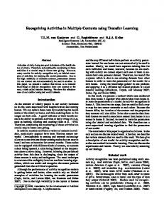
Figure 1: Left: key frames of activities “hurdle race” (top) and “long jump” (bottom); Right: attribute transition probabilities of the two activities (“hurdle race” / “long jump”) for attributes “run”, “jump”, and “land”.
The work also suggests that, for action categorization, supervised attribute learning is far more useful than unsupervised learning, resembling a similar observation from image recognition [20]. However, all of these representations are BoF-like, in the sense that they represent actions as orderless feature collections, reducing an entire video sequence to an attribute vector. For this reason, we denote them holistic attribute representations. The temporal evolution of semantic concepts, throughout a video sequence, has not yet been exploited as a cue for action understanding. There has, however, been some progress towards this type of modeling in the text analysis literature, where temporal extensions of latent Dirichlet allocation (LDA) have been proposed. Two representatives are the dynamic topic model (DTM) [23] and the topic over time (TOT) model [24]. Although modeling topic dynamics, these models are not necessarily applicable to semantic action recognition. First, like the underlying LDA, they are unsupervised models, and thus likely to underperform in recognition tasks [11, 10]. Second, the joint goal of topic discovery and modeling topic dynamics requires a complex graphical model. This is at odds with tractability, which is usually achieved by sacrificing the expressiveness of the temporal model component.
3
Modeling the Dynamics of Activity Attributes
In this section, we introduce a new model, the binary dynamic system, for joint representation of the distribution and dynamics of activities in action attribute space. 3.1
Semantic Representation
Semantic representations characterize video as a collection of descriptors with explicit semantics [10, 11]. They are obtained by defining a set of semantic concepts (or attributes, scene classes, etc), and learning a classifier to detect each of those concepts. Given a video v ∈ X to analyze, each classifier produces a confidence score for the presence of the associated concept. The ensemble of classifiers maps the video to a semantic space S, according to π : X → S = [0, 1]K , π(v) = (π1 (v), · · · , πK (v))T , where πi (v) is the confidence score for the presence of the i-th concept. In this work, the classification score is the posterior probability of a concept c given video v, i.e., πc (v) = p(c|v) under a certain video representation, e.g., the popular BoF histogram of spatiotemporal descriptors. As the video sequence v progresses with time t, the semantic encoding defines a trajectory {π t (v)} ⊂ S. The benefits of semantic representations for recognition, namely a higher level of abstraction (which leads to better generalization than appearance-based representations), substantial robustness to the performance of the visual classifiers πi (v), and intrinsic ability to account for contextual relationships between concepts, have been previously documented in the literature [13]. No attention has, however, been devoted to modeling the dynamics of semantic encodings of video. Figure 1 motivates the importance of such modeling for action recognition, by considering two activity categories (“long jump” and “hurdle race”), which involve the same attributes, with roughy the same probabilities, but span very different trajectories in S. Modeling these dynamics can substantially enhance the ability of a classifier to discriminate between complex activities. 3.2
Binary PCA
The proposed representation is a generalization of binary PCA [14], a dimensionality reduction technique for binary data, belonging to the generalized exponential family PCA [25]. It fits a linear model to binary observations, by embedding the natural parameters of Bernoulli distributions in a low-dimensional subspace. Let Y denote a K × τ binary matrix (Ykt ∈ {0, 1}, e.g., the indicator of 3
occurrence of attribute k at time t) where each column is a vector of K binary observations sampled from a multivariate Bernoulli distribution ykt Ykt ∼ B(ykt ; πkt ) = πkt (1 − πkt )1−ykt = σ(θkt )ykt σ(−θkt )1−ykt , ykt ∈ {0, 1}.
(1)
π log( 1−π )
The log-odds θ = is the natural parameter of the Bernoulli distribution, and σ(θ) = (1 + e−θ )−1 is the logistic function. Binary PCA finds a L-dimensional (L � K) embedding of the natural parameters, by maximizing the log-likelihood of the binary matrix Y i X h L = log P (Y ; Θ) = Ykt log σ(Θkt ) + (1 − Ykt ) log σ(−Θkt ) (2) k,t
under the constraint K×L
Θ = CX + u1T , L×τ
K
(3)
τ
where C ∈ R ,X ∈R , u ∈ R and 1 ∈ R is the vector of all ones. Each column of C is a basis vector of a latent subspace and the t-th column of X contains the coordinates of the t-th binary vector in this basis (up to a translation by u). Binary PCA is not directly applicable to attribute-based recognition, where the goal is to fit the vectors of confidence scores {π t } produced by a set of K attribute classifiers (and not a sample of binary attribute vectors per se). To overcome this problem, we maximize the expected log-likelihood of the data Y (which is the lower bound to the log expected likelihood of the data Y , by Jensen’s inequality). Since E[y t ] = π t , it follows from (2) that i X h EY [L] = πkt log σ(Θkt ) + (1 − πkt ) log σ(−Θkt ) . (4) k,t
The proposed extension of binary PCA consists of maximizing this expected log-likelihood under the constraint of (3). It can be shown that, in the absence of the constraint, the maximum occurs when σ(Θkt ) = πkt , ∀k, t. As in PCA, (3) forces σ(Θkt ) to lie on a subspace of S, i.e., σ(Θkt ) = π ˆkt ≈ πkt .
(5)
The difference between the expected log-likelihood of the true scores {π t } and the binary PCA scores {σ(θ t ) = σ(Cxt + u)} (σ(θ) ≡ [σ(θ1 ), · · · , σ(θK )]T ) is E[∆L({π t }; {σ(θ t )})]
= = =
� � � � EY log(P (Y ; {π t })) − EY log(P (Y ; {σ(θ t )})) � X � πkt 1 − πkt πkt log + (1 − πkt ) log k,t σ(Θkt ) σ(−Θkt ) X KL[B(y; π t )||B(y; σ(θ t ))], t
(6) (7) (8)
where KL(B(y; π)||B(y; π 0 )) is the Kullback-Leibler (KL) divergence between two multivariate Bernoulli distributions of parameters π and π 0 . By maximizing the expected log-likelihood (4), the optimal projection {θ ∗t } of the attribute score vectors {π t } on the subspace of (3) also minimizes the KL divergence of (8). Hence, for the optimal natural parameters {θ ∗t }, the approximation of (5) is the best in the sense of KL divergence, the natural similarity measure between probability distributions. 3.3
Binary Dynamic Systems
A discrete time linear dynamic system (LDS) is defined by � xt+1 = Axt + v t , y t = Cxt + wt + u L
K
(9)
where xt ∈ R and y t ∈ R (of mean u) are the hidden state and observation variable at L×L time t, respectively; A ∈ R is the state transition matrix that encodes the underlying dynamK×L ics; C ∈ R the observation matrix that linearly maps the state to the observation space; and x1 = µ0 + v 0 ∼ N (µ0 , S0 ) an initial condition. Both state and observations are subject to additive Gaussian noise processes v t ∼ N (0, Q) and wt ∼ N (0, R). Since the noise is Gaussian and L < K, the matrix C can be interpreted as a PCA basis for the observation space (L eigenvectors of the observation covariance). The state vector xt then encodes the trajectory of the PCA coefficients (projection on this basis) of the observed data over time. This interpretation is, in fact, at the core of the popular dynamic texture (DT) [15] representation for video. While the LDS parameters 4
Algorithm 1: Learning a binary dynamic system Input : a sequence of attribute score vectors {π t }τt=1 , state space dimension n. τ Binary PCA: {C, X, u} = B-PCA({π t }t=1 , n)� using the method of [14]. � t2 Estimate state parameters (Xt1 ≡ xt1 , · · · , xt2 ): 1 A = X2τ (X1τ −1 )† ; V = (X)τ2 − A(X)τ1 −1 ; Q = τ −1 V (V )T ; Pτ Pτ 1 1 T µ0 = τ t=1 xt ; S0 = τ −1 t=1 (xt − µ0 )(xt − µ0 ) .
Output: {A, C, Q, u, µ0 , S0 } can be learned by maximum likelihood, using an expectation-maximization (EM) algorithm [26], the DT decouples the learning of observation and state variables. Observation parameters are first learned by PCA, and state parameters are then learned with a least squares procedure. This simple approximate learning algorithm tends to perform very well, and is widely used in computer vision. The proposed binary dynamic system (BDS) is defined as � xt+1 = Axt + v t , y t ∼ B(y; σ(Cxt + u)) L
(10)
K
where xt ∈ R and u ∈ R are the hidden state variable and observation bias, respectively; A ∈ RL×L is the state transition matrix; and C ∈ RK×L the observation matrix. The initial condition is given by x1 = µ0 + v 0 ∼ N (µ0 , S0 ); and the state noise process is v t ∼ N (0, Q). Like the LDS of (9), the BDS can be interpreted as combining a (now binary) PCA observation component with a Gauss-Markov process for the state sequence. As in binary PCA, for attribute-based recognition the binary observations y t are replaced by the attribute scores π t , their log-likelihood under (10) by the expected log-likelihood, and the optimal solution minimizes the approximation of (5) for the most natural definition of similarity (KL divergence) between probability distributions. This is conceptually equivalent to the behavior of the canonical LDS of (9), which determines the subspace that best approximates the observations in the Euclidean sense, the natural similarity measure for Gaussian data. Note that other extensions of the LDS, e.g., kernel dynamic systems (KDS) that rely on a non-linear kernel PCA (KPCA) [27] of the observation space but still assume an Euclidean measure (Gaussian noise) [28, 6], do not share this property. We will see, in the experimental section, that the BDS is a better model of attribute dynamics. 3.4
Learning
Since the Gaussian state distribution of an LDS is a conjugate prior for the (Gaussian) conditionaldistribution of its observations given the state, maximum-likelihood estimates of LDS parameters are tractable. The LDS parameters ΩLDS = {A, C, Q, R, µ0 , S0 , u} of (9) can thus be estimated with an EM algorithm [26]. For the BDS, where the state is Gaussian but the observations are not, the expectation step is intractable. Hence, approximate inference is required to learn the parameters ΩBDS = {A, C, Q, µ0 , S0 , u} of (10). In this work, we resort to the approximate DT learning procedure, where observation and state components are learned separately [15]. The binary PCA basis is learned first, by maximizing the expected log-likelihood of (4) subject to the constraint of (3). Since the Bernoulli distribution is a member of exponential family, (4) is concave in Θ, but not in C, X and u jointly. We rely on a procedure introduced by [14], which iterates between the optimization with respect to one of the variables C, X and u, with the remaining two held constant. Each iteration is a convex sub-problem that can be solved efficiently with a fixed-point auxiliary function (see [14] for details). Once the latent embedding C ∗ , X ∗ and u∗ of the attribute sequence in the optimal subspace is recovered, the remaining parameters are estimated by solving a leastsquares problem for A and Q, and using standard maximum likelihood estimates for the Gaussian parameters of the initial condition (µ0 and S0 ) [15]. The procedure is summarized in Algorithm 1.
4
Measuring Distances between BDSs
The design of classifiers that account for attribute dynamics requires the ability to quantify similarity between BDSs. In this section, we derive the BDS counterpart to the popular Binet-Cauchy kernel (BCK) for the LDS, which evaluates the similarity of the output sequences of two LDSs. Given 5
LDSs Ωa and Ωb driven by identical noise processes v t and wt with observation sequences y (a) and y (b) , [16] propose a family of BCKs hX∞ i (a) (b) KBC (Ωa , Ωb ) = Ev,w e−λt (y t )T W y t , (11) t=0
where W is a semi-definite positive weight matrix and λ > 0 a temporal discounting factor. To (a) (b) extend (11) to BDSs Ωa and Ωb , we note that (y t )T W y t is the inner product of an Euclidean (a) (b) (a) (b) (a) (b) output space of metric d2 (y t , y t ) = (y t − y t )T W (y t − y t ). For BDSs, whose obser(a) (b) vations y t are Bernouli distributed with parameters {σ(θ t )}, for Ωa , and {σ(θ t )}, for Ωb , this distance measure is naturally replaced by the KL divergence between Bernoulli distributions " DBC (Ωa , Ωb ) = Ev
∞ X
−λt
e
�
(a) (b) KL(B(σ(θ t ))||B(σ(θ t )))
+
�
#
(b) (a) KL(B(σ(θ t ))||B(σ(θ t )))
t=0
= Ev
(12)
�X ∞ t=0
−λt
e
� �T � �� (a) (b) (a) (b) σ(θ t ) − σ(θ t ) θt − θt ,
where θ t = Cxt + u. The distance term at time t can be rewritten as (a)
(b)
(a)
(σ(θ t ) − σ(θ t ))T (θ t
(a)
(b)
− θ t ) = (θ t
(b) (b) ˆ t (θ (a) − θ t ), − θ t )T W t
(13)
ˆ t a diagonal matrix whose k-th diagonal element is W ˆ t,k = (σ(Θ(a) ) − σ(Θ(b) ))/(Θ(a) − with W t,k t,k t,k (b) ˆ (a,b) ) (where, by the mean value theorem, Θ ˆ (a,b) is some real value between Θ ˆ (a) and Θ ) = σ 0 (Θ t,k
t,k
t,k
t,k
ˆ (b) ). This reduces (13) to a form similar to (11), although with a time varying weight matrix Wt . Θ t,k It is unclear whether (12) can be computed in closed-form. We currently rely on the approximation P∞ ¯ (a) ) − σ(θ ¯ (b) ))T (θ ¯ (a) − θ ¯ (b) ), where θ ¯ is the mean of θ. DBC (Ωa , Ωb ) ≈ t=0 e−λt (σ(θ t t t t
5
Experiments
Several experiments were conducted to evaluate the BDS as a model of activity attribute dynamics. In all cases, the BoF was used as low-level video representation, interest points were detected with [2], and HoG/HoF descriptors [3] computed at their locations. A codebook of 3000 visual words was learned via k-means, from the entire training set, and a binary SVM with histogram intersection kernel (HIK) and probability outputs [29] trained to detect each attribute using the attribute definition same as [11]. The probability for attribute k at time t was used as attribute score πtk , which was computed over a window of 20 frames, sliding across a video. 5.1
Weizmann Activities
To obtain some intuition on the performance of different algorithms considered, we first used complex activity sequences synthesized from the Weizmann dataset [17]. This contains 10 atomic action classes (e.g., skipping, walking) annotated with respect to 30 lower-level attributes (e.g., “one-armmotion”), and performed by 9 people. We created activity sequences by concatenating Weizmann actions. A sequence of degree n (n = 4, 5, 6) is composed of n atomic actions, performed by the same person. The row of images at the top of Figure 2 presents an example of an activity sequence of degree 5. The images shown at the top of the figure are keyframes from the atomic actions (“walk”, “pjump”, “wave1”, “wave2”, “wave2”) that compose this activity sequence. The black curve (labeled “Sem. Seq”) in the plot at the bottom of the figure shows the score of the “two-arms-motion” attribute, as a function of time. 40 activity categories were defined per degree n (total of 120 activity categories) and a dataset was assembled per category, containing one activity sequence per person (9 people, 1080 sequences in total). Overall, the activity sequences differ in the number, category, and temporal order of atomic actions. Since the attribute ground truth is available for all atomic actions in this dataset, it is possible to train clean attribute models. Hence, all performance variations can be attributed to the quality of the attribute-based inference of different approaches. We started by comparing the binary PCA representation that underlies the BDS to the PCA and KPCA decompositions of the LDS and KDS. In all cases we projected a set of attribute score vectors ˆ t }, and {π t } into the low-dimensional PCA subspace, computed the reconstructed score vectors {π ˆ t ), as reported in Figure 3. The kernel used for KPCA was the KL divergence KL(B(y, π t )||B(y, π 6
6
#
0
!%#
PCA kernel−PCA binary−PCA
4
>?1 !%!'
7?1 78 >?1
!%&
!%!&
78 7?1
4/56078
)**+,-.*/0123+/
!%!(
;3