May 11, 2012 - entific research documents, whether they are pub- lished or not. ... motion signatures (LMSs) of HOG descriptors introduced by [1]. Our main ...
Recognizing Gestures by Learning Local Motion Signatures of HOG Descriptors Mohamed-B´echa Kaˆaniche (Sup’Com - TUNISIA), and Franc¸ois Br´emond (INRIA - FRANCE) February 22, 2012 Abstract We introduce a new gesture recognition framework based on learning local motion signatures (LMSs) of HOG descriptors introduced by [1]. Our main contribution is to propose a new probabilistic learning-classification scheme based on a reliable tracking of local features. After the generation of these LMSs computed on one individual by tracking Histograms of Oriented Gradient (HOG) [2] descriptor, we learn a code-book of video-words (i.e. clusters of LMSs) using kmeans algorithm on a learning gesture video database. Then the video-words are compacted to a code-book of code-words by the Maximization of Mutual Information (MMI) algorithm. At the final step, we compare the LMSs generated for a new gesture w.r.t. the learned code-book via the k-nearest neighbors (k-NN) algorithm and a novel voting strategy. Our main contribution is the handling of the N to N mapping between code-words and gesture labels within the proposed voting strategy. Experiments have been carried out on two public gesture databases: KTH [3] and IXMAS [4]. Results show that the proposed method outperforms recent state-of-the-art methods.
1
Introduction
Gesture recognition from video sequences is one of the most important challenges in computer vision and behavior understanding since it enables to interact with some human machine interfaces (HMI) or to monitor complex human activities. More precisely, it is considered as the bottleneck for precise human behavior understanding. Indeed, in order to detect sophisticated behavior, we need to analyze human gestures and interactions. So, the efficiency and the effectiveness of the gesture recognizer influence those of the behavior understanding process. The main challenge for recognizing gestures from video sequences is to cope with the large variety of gestures. Recognizing gestures involves handling a considerable number of degrees of freedom (DoF), huge variability of the 2D appearance depending on the camera view point (even for the same gesture), different silhouette scales (i.e. spatial resolution) and many resolutions for the temporal dimension (i.e. variability of the gesture speed). 1
There are two main categories of techniques in gesture recognition: (1) postureautomaton model techniques where the spatial (posture or appearance features) and the temporal aspects are modeled separately and (2) motion model techniques where there is a unique spatio-temporal model. The former techniques [5, 6] use a recognition process composed of a single stage where the parameters of the real target are extracted and then fitted to the adequate gesture model (composed of posture/appearance states and transitions between them). The model fitting is driven by the attempt to minimize a residual measure between the projected model and the person contours (e.g. edges of the body) which requires a very good segmentation of body parts. Thus, such techniques require video sequences without very strong noise. In addition, the gesture model must be modified when a new gesture needs to be recognized. Moreover, the computational complexity of such approaches is generally huge since it is proportional to the number of gestures to be recognized However, the latter techniques [7, 8] have gained more and more popularity since they use a two stage recognition technique based on learning motion and then classifying unknown ones. Such techniques are more robust to noise and segmentation quality while they still brittle due to illumination variability and occlusions. Also, adding a new gesture is easier since you just have to update the learned database. Therefore, it is crucial to detect motion features that account and describe more faithfully the concerned gesture. use a unique motion model consisting of sparse spatio-temporal descriptors Global motion descriptors or local motion descriptors can be selected depending on the type of video. In this paper, we propose a new learning-classification framework for gesture recognition [9] using local motion signatures [1] of HOG descriptors as a gesture representation. The developed framework is designed to cope with efficiency-effectiveness trade-off. First, we compute for each detected individual in the scene a set of features (i.e. corner points). For each feature, we associate a 2D descriptor (i.e. Histograms of Oriented Gradients (HOG) [2]), which is tracked over time to build a reliable local motion signature. Thus a gesture is represented as a set of local motion signatures. Second, we learn the local motion signatures for a given set of gestures by clustering them into local motion patterns (i.e. clusters). Last, we classify the gesture of a person in a new video by extracting the person local motion signatures and voting for the most likely gesture w.r.t. learned local motion patterns. The approach has been validated on two public gesture databases: KTH [3] and IXMAS [4] and results demonstrate an improvement over recent state-of-the-art methods. The remaining of this paper is structured into six parts. The next section overviews the state-of-the-art in gesture recognition. Section 3 summarizes the building process of local motion signatures. Section 4 presents the learning stage and section 5 details the classification stage. Results are described and discussed in section 6. Finally, section 7 concludes this paper by over-viewing the contributions and exposing future work.
2
Previous Work
In this section, we focus on over-viewing the state-of-the-art of motion model based gesture recognition algorithms which contains two main categories: (1) global motion 2
based methods and (2) local motion based methods. For global motion based methods, [10] have proposed to encode an action by an “action sketch” extracted from a silhouette motion volume obtained by stacking a sequence of tracked 2D silhouettes. The “action sketch” is composed of a collection of differential geometric properties (e.g. peak surface, pit surface, ridge surface) of the silhouette motion volume. For recognizing an action, the authors use a learning approach based on a distance and epipolar geometrical transformation for viewpoint changes. Lu and Little[11] propose to recognize gestures via maximum likelihood estimation with Hidden Markov Models and a global HOG descriptor computed over the whole body. The authors extend their method in [12] by reducing the global descriptor size with principal component analysis. [13] extract space-time saliency, space-time orientations and weighted moments from the silhouette motion volume. Gesture classification is performed using nearest neighbors algorithm and Euclidean distance. Recently, [7] introduce action signatures. An action signature is a 1D sequence of angles (forming a trajectory) which are extracted from a 2D map of adjusted orientation of the gradients of the motion-history image. A similarity measure is used for clustering and classification. As these methods are using global motion, they strongly depend on the segmentation quality of the silhouette which influences the robustness of the classification. Furthermore, local motion, which can help to discriminate similar gestures, can easily get lost with a noisy video sequence or with repetitive self-occlusions. Local motion based methods overcome these limits by considering sparse and local spatio-temporal descriptors more robust to short occlusions and to noise. For instance, [14] introduce the bag of word paradigm for motion recognition with unsupervised learning of local features: space-time interest points. Similarly, [15] propose a 3-D (2D + time) SIFT descriptor and apply it to action recognition using the bag of word paradigm. Schuldt et al.[3] propose to use Support Vector Machine classifier with local space-time interest points for gesture categorization. [16] introduce local motion histograms and use an Ada-boost framework for learning action models. More recently, [8] apply Support Vector Machine learning on correlogram and spatial temporal pyramid extracted from a set of video-word clusters of 3D interest points. These methods are generally not robust enough since the temporal local windows (with short size and fixed spatial position) do not model the exact local motion but arbitrarily several slices of that motion instead. To go beyond the state of the art, we propose a novel gesture learning-classification framework based on learning local motion signatures which are built thanks to tracking local HOG descriptors over sufficiently long period of time. The proposed gesture representation combines the advantages of global and local gesture motion approaches in order to improve the recognition quality. Indeed, instead of using local video patches which capture only snapshots of local motion, we track local features in order to capture the whole local motion for each feature point. Simultaneously to our work, several similar approaches have been proposed but with different technical frameworks. For instance, [17] describe a method for action recognition using hierarchical spatio-temporal context modeling with three levels : (1) a feature point descriptor based on SIFT, (2) a trajectory transition descriptor and (3) a trajectory proximity descriptor. Multiple-Kernel Learning is then used for pruning. [18] use a region descriptor composed of two sub-descriptors (the first one is based on 3
SIFT and the second one is based on RGB colors) with a an euclidean distance based similarity measure and an energy minimization technique to build large displacement Optical Flow for human motion analysis. [19] propose a feature tree of spatio-temporal feature points for action representation. The recognition of an action is done by retrieving the nearest neighbor for a query feature and then applying a voting mechanism. [20] introduce a new descriptor based on velocity history of tracked Shi-Tomasi feature points (with KLT algorithm). To recognize activities, a markov chain model is used with an Expectation Maximization (EM) process for training and conditional probability maximization for classification. Similarly, [21] define trajectons which are quantized trajectory snippets of Shi-Tomasi tracked feature points. A bag of words training step along with a Support Vector Machine (SVM) based classification step are used for motion categorization. Lately, [22] build a descriptor dictionary based on the average of oriented gradients and the average of optical flow. Agglomerative clustering and k-medoids are used for building clusters and Support Vector Machine (SVM) is used for classification. Latterly, [23] use a Hough-transform based voting framework by training random trees in order to find a mapping between 3D feature patches (i.e. cuboids) and their votes in the Hough space. The classification is based on the multi-class classifier based on the leaves of the trees. Compared to these works, we believe that our method tackle the recognition problem differently. First, our recognition process is based on the assumption that a gesture is composed of three phases: (1) pre-stroke, (2) stroke and (3) post-stroke; as claimed by [24]. Each phase has different motion patterns compared to other phases. So, we rely on the feature orientation trajectory representation (combining local and global motion information), the dimensional reduction (which is done with PCA by selecting only the most important motion information) and the learning algorithm (tuned to form a meaningful number of motion clusters according to the number of gestures to be recognized), in order to identify the three motion clusters for each gesture. In such way, similar gestures can share one or two motion clusters but not more. Second, we use a people detection step (using background subtraction) in order to reduce noisy motion: only motions relative to human being actions are detected. Finally, we use a probability inference framework with weighted voting scheme for classification process. This framework handle the many-to-many mapping between gesture labels and motion clusters. This contrast with classical methods which use a one-to-many mapping or feature-tree based classifiers (e.g. [19],[23]). In addition, the proposed classifier can handle the differentiation between similar gestures and gives a recognition likelihood for each of them.
3
Local Motion Signatures Generation
Our gesture representation is a set of Local Motion Signatures (LMSs) which are generated through four steps: (1) People Detection/Feature Selection, (2) HOG Descriptor Generation, (3) Feature/HOG descriptor Tracking and (4) LMSs extraction.
4
3.1
People Detection and Feature Selection
People detection is performed by background subtraction to determine moving regions followed by a morphological dilation [25]. Then a people classifier is applied to determine bounding boxes around single individuals. The people bounding boxes define a mask for feature point extraction. This step not only limits the search space for feature points but also separates distinct moving regions: corresponding to different individuals. This enables to apply the gesture recognition process to different people until they overlap each other. Feature selection is then performed for each detected person using Shi-Thomasi corner detector [26] or Features from Accelerated Segment Test (FAST) corner detector [27]. Then corner points are sorted in decreasing order according to the corner strength. After that, we select the most significant corners by ensuring a minimum distance among them. Thus, feature points enable us to localize points where HOG descriptors can be computed since they usually correspond to locations where motion can be easily discernible.
3.2
HOG Descriptor Generation
For each feature point, we compute a local HOG descriptor [2] from a descriptor block composed of 3 × 3 cells; each of them having a pixel size of 5 × 5: The feature point is the center of the central cell of the block. The gradient magnitude g and the gradient orientation θ are computed for all the pixels in the block using respectively equation 1 and equation 2 from the image gradients computed by simple 1D-filters (gx and gy ). q (1) g(u, v) = gx (u, v)2 + gy (u, v)2 gy (u, v) gx (u, v)
θ(u, v) = arctan
(2)
For each cell cij where (i, j) ∈ {1, 2, 3}2 in the block, we compute a feature vector fij by quantizing the unsigned orientation into K orientation bins weighted by the gradient magnitude as defined by equation 3. fij = [fij (β)]Tβ∈[1..K] where fij (β) is defined by equation 4. X fij (β) = g(u, v) δ[bin(u, v) − β]
(3)
(4)
(u,v)∈cij
The function bin(u, v) returns the index of the orientation bin associated to the pixel (u,v) and the function δ[] is the Kronecker delta. Therefore, the 2D descriptor of the block is a vector concatenating the feature vectors of all its cells normalized by the coefficient ρ which is defined in equation 5. ρ=
3 X 3 X K X
fij (β)
i=1 j=1 β=1
5
(5)
Figure 1: HOG Descriptor tracking using extended Kalman filter Each cell encapsulates a local and specific information about the 2D descriptor which increases its trackability.
3.3
Feature/HOG descriptor Tracking
Let us suppose that we have detected a feature point and associated to it a HOG descriptor dt−1 in the frame ft−1 , we are now interested to determine the descriptor dt in the frame ft which can be identified to dt−1 (the center of that descriptor can be identified to the previous feature point). The basic idea is to minimize a quadratic error function E(dt , dt−1 ) in a neighborhood Vft in the frame ft corresponding to the predicted position of dt−1 obtained by an extended Kalman filter. In the case when several descriptors (d1t , d2t , ..., dkt ) in this neighborhood satisfy the minimum of the error function, we compute the visual evidence (intensity difference in gray-scale) between each descriptor and the descriptor of the previous frame to track dt−1 . The tracker will choose the descriptor that has the nearest visual evidence to dt−1 .. A newly computed descriptor initializes a new tracking process through the extended Kalman filter. For a tracked HOG descriptor dt−1 in the frame ft−1 , we determine the descriptor dt in the frame ft which can be identified to dt−1 through the “Predict” and “Correct” stages of the Kalman filter. When a descriptor is lost, it may be replaced by a new computed descriptor associated to a newly detected corner. Fig. 1 illustrates the tracking algorithm of HOG Descriptors. In the following, we describe respectively the Kalman filtering with descriptor metrics and the effective HOG descriptor tracking algorithm (actually performing the measurement after prediction and before correction).
6
3.3.1
Kalman Filtering and Descriptor Metrics
In order to track the descriptor position, we use a Kalman filter with a linear randomwalk motion model for prediction. The basic idea of a Kalman filtering based tracker is to recursively estimate the state vector given the last estimate and a new measurement which is made by the traditional tracker. The state vector X used by the Kalman filter is defined by equation 6. X = [ px py vx vy d ]T (6) where (px , py ) is the position of the descriptor, (vx , vy ) is its velocity and dˆ is the descriptor value. A candidate descriptor (which has not been tracked yet) is described by a measurement vector Z as defined in equation 7. Z = [ p x p y d ]T
(7)
When a corner point is newly detected and its correspondent descriptor is computed (first appearance of the individual or replacing a lost descriptor), the Kalman filter is initialized with the state X (0) with the speed of the individual centroid and with the initial covariance matrix P (0) using large variances for the speed. At each tracking step, the Kalman filter predicts a state Xˆ (t) from the previous actual state Xˆ (t−1) and the motion model. Using the predicted state and the apriori covariance matrix, the HOG tracking algorithm returns the actual current measure to the filter. Finally, the filter computes the actual current state by updating the predicted state with the innovation between the actual measure and the predicted measure. Hereafter, the static filtering of the descriptor is detailed. First of all, we define an error function E that measures the dissimilarity between two given descriptors d(n) and d(m) according to equation 8: E(d(n) , d(m) ) =
9×K X
(n)
(di
(m) 2
− di
)
(8)
i=1 (n)
(m)
where di and di are respectively the ith component of the descriptors d(n) and d(m) . We want to calculate the estimate dˆ such that the least square error between past measurements (i.e. d(1) , ..., d(t) ) and the descriptor value d of the state vector is minimum. The solution for this minimization problem is given by this equation: t
1 X (i) d dˆ = t i=1
(9)
Since we aim to have an estimate of the state of the descriptor at each step of the tracking, we use the recursive least square method by using the results of equation 10. Gain
dˆ(t) = |{z}
actual state
measure z}|{ Actual measure Predicted z }| { z}|{ 1 ˆ(t−1) d dt − dˆ(t−1) ) | {z } + t |( {z }
predicted state
(10)
Innovation
Here the gain specifies how much do we pay attention to the difference between what we expected and what we actually get. Note that the gain decreases while the tracking advance which means that we become more and more confident in the descriptor 7
estimation while the tracking progress. To decide whether the descriptor is correctly tracked, the following constraint should be verified: E(dˆ(t) , dˆ(1) ) ≤
9×K 100
(11)
where the constant 9/100 is set empirically. In order to compute the actual measure, the HOG tracking algorithm needs two metrics: A distance between a state vector and a measurement vector and a confidence measure between these two vectors. Equation 12 defines a distance D between a candidate descriptor Z in the current frame and a tracked descriptor X through previous frames. p E(Zd , Xd ) ||Zp − Xp || +γ (12) D(Z, X ) = α p σp σd ||Zd || + ||Xd || + 1 where α and γ are empirically derived weight parameters, Zd , Xd , Zp , Xp are respectively the estimated value and the descriptor position of Z and X , and σd and σp are the covariance parameters extracted from the Kalman filter’s covariance matrix. The first term of the distance represents the scaled difference between the two descriptor values and the second term represents the difference between the candidate and predicted descriptor location. The confidence C in the candidate descriptor Z to correspond to the tracked descriptor X is defined by equation 13. C(Z, X ) = 3.3.2
1 1 + D(Z, X )
(13)
The HOG Descriptor Tracking Algorithm
The tracking algorithm consists in a downhill search around the predicted position by minimizing the quadratic error function E. Thus, we determine search regions for next measurements using last states, predicted states and uncertainties and then we get new measurements in the search regions. Note that as a preliminary stage, all positions in the search area are used to compute the candidate descriptors. The confidence measure (as defined in equation 13) is used to select the best solution, if the downhill search gives several solutions. For each descriptor, the tracking algorithm of 2D HOG descriptors is run as described hereafter. Where the ellipse procedure returns the ellipse with foci (Xˆ (t−1) , Xˆ (t) ) and eccentricity e defined by equation 14. e=
c a
(14)
where c is the focal distance and a is the semi-major axis of the ellipse which is computed as defined by formula 15. p a = c2 + b2 (15) where b is the semi-minor axis computed as defined by formula 16. q b = c + σx2 + σy2 8
(16)
Algorithm 1 2D HOG descriptor tracking algorithm Require: Xˆ (t−1) , Xˆ (t) , Pt− {Last estimated state, predicted state and error covariance matrix} Ensure: Z (t) {The actual measure} − 1: R ← ellipse(Xˆ (t−1) , Xˆ (t) , Pt ) {Compute the search region} 2: S ← ∅ {Initialize the set of candidate measures} 3: for all Z ∈ R do K then 4: if E(Z, Xˆ (t) ) < 9100 5: S ← S ∪ {Z} 6: end if 7: end for 8: maxConf idence ← 0 9: for all Z ∈ S do ˆ (t) Xˆ (t−1) ) 10: conf idence ← C(Z,X )+C(Z, 2 11: if conf idence > maxConf idence then 12: maxConf idence ← conf idence 13: Z (t) ← Z 14: end if 15: end for where σx and σy are the variance extracted from the covariance matrix Pt− of√the Kalman filter. Note that b ≥ c which implies that b2 + c2 > 2 c2 and thus a ≥ 2 c (using equation 15). This ensures that the search region has a minimum size according to the focal distance which is the half of the predicted motion of the descriptor.
3.4
LMSs extraction
For each tracked HOG descriptor, we associate to it a temporal HOG descriptor from which we extract a local motion signature (LMS) by applying several normalizations. The temporal HOG descriptor is the vector obtained by the concatenation of the final descriptor estimate dˆ and the positions of the descriptor during the tracking process. The dimension of this vector is 9 × K + 2 × ` where ` is the number of the 2D tracked positions. If we assume that T d = [(x1 , y1 ), ..., (x` , y` )]T is the array of the descriptor d locations, then the temporal HOG descriptor is the heterogeneous vector V = [dˆ T d ]T . Given the tracked position vector T d , we define the line trajectory vector L as: Ld = [(w1 , h1 ), ..., (w`−1 , h`−1 )]T (17) where wi = xi+1 − xi and hi = yi+1 − yi . The trajectory orientation vector Θd = [θ1 , ..., θ`−2 ]T is computed thanks to the formula defined by equation 18. ∀i ∈ [1, ` − 2]; θi = arctan(hi+1 , wi+1 ) − arctan(hi , wi )
(18)
where the arctan function returns the orientation of the given line with respect to the x axis. Since −2π ≤ θi ≤ 2π, we normalize the vector by dividing all its components ˜ d . The local motion descriptor is defined as by 2π. The resulting vector is noted Θ 9
the concatenation of the descriptor estimation dˆ which indicates the texture involved ˜ d which represents the in the motion and the normalized trajectory orientation vector Θ motion. Its dimension is 9 × K + ` − 2. To reduce the dimension of the local motion descriptor, we apply Principal Component Analysis (PCA) and project the θi on the three first principal axis θˆ1 , θˆ2 , θˆ3 . Since PCA cannot handle trajectories of different length, we first extract all sub-trajectories of length 3 from available trajectories by slicing them. These sub-trajectories are used to feed the PCA process. Thus we get a ˆ d = [d θˆ1 θˆ2 θˆ3 ]T . Compared to the global PCA-HOG final local motion descriptor Θ descriptor proposed by [12] (one global HOG descriptor for each gesture/action), the proposed gesture/action descriptor consists in a set of local motion descriptors which accounts more faithfully for local motion. Instead of computing a global HOG volume from a person already tracked, we use local HOGs tracked independently. Our method contrasts from traditional local motion methods by using the tracking process of 2D descriptors instead of 2D descriptor time-volume.
4 4.1
Gesture Learning K-means Clustering
For learning gestures, we assume that the training data-set is built with videos, each of them containing one and only one gesture instance. For each training video sequence, LMSs are extracted and annotated with the corresponding gesture label. Then, we apply the k-means algorithm in order to group these LMSs into clusters called videowords which are the local motion patterns. The similarity measure used for comparing two different LMSs in k-means is the Euclidean distance. Indeed we have carried out different experiments with different distances and found out that the euclidean distance gives the best results. Thus, given as input the set S of annotated local motion signatures generated with all the training videos, the k-means algorithm outputs k video-words Si , i = 1, 2, ..., k. The value of k is empirically chosen so that is large enough to describe correctly the set of the m gestures to learn (k > 3 × m). The lower bound for choosing of k is justified by analyzing the videos illustrating gestures [24]: gestures are usually composed of three units of coherent motion (i.e. pre-stroke, stroke and post-stroke) and in our representation, these units of motion correspond to local motion patterns. Thanks to the cluster membership map provided by the k-means algorithm, we annotate each video-word with the gesture labels associated with the LMSs of this cluster.
4.2
Maximization of Mutual Information
Once we have obtained the video-words, an optional step is to reduce their dimensionality by compacting them into code-words. To achieve this goal, we propose to apply Maximization of Mutual Information (MMI) algorithm [8] on the clusters generated by the k-means algorithm. Let C be the centroids of the generated clusters C ∈ C = [µ1 ..µk ]. Let G be the gesture labels G ∈ G = [g1 ..gm ]. With the cluster membership map A : S → C, we define the conditional probability distributions
10
P (C|G) and P (G|C) by equations 19 and 20. P (C = µi |G = gi ) =
Card(Label−1 (gi ) ∩ A−1 (µi )) Card(Label−1 (gi ))
(19)
P (G = gi |C = µi ) =
Card(Label−1 (gi ) ∩ A−1 (µi )) Card(A−1 (µi ))
(20)
Where the function Label is the map between feature LMSs and gesture labels; Card(.) is the cardinal operator. By taking as definition of the marginal distributions of C and G the formulas 22 and 23, we can verify that these definitions (i.e. equations 19 and 20) match the conditional probability definition (c.f . equation 21). P (G = gi , C = µi ) P (C = µi ) P (C = µi |G = gi ) P (G = gi ) = P (C = µi )
P (G = gi |C = µi ) =
Card(A−1 (µi )) Card(S)
(22)
Card(Label−1 (gi )) Card(S)
(23)
P (C = µi ) = P (G = gi ) =
(21)
Thus, we can deduce the joint distribution of C and G from equation 21 which gives: P (G = gi , C = µi ) =
Card(Label−1 (gi ) ∩ A−1 (µi )) Card(S)
(24)
Hence, the mutual information between C and G which measures how much information from C is contained in G is: M I(C, G) = X
P (C = µi , G = gi ) log
µi ∈C,gi ∈G
P (C = µi , G = gi ) P (C = µi )P (G = gi )
(25)
The goal of MMI algorithm is to reduce incrementally the size of the video-words ˆ G) C in order to obtain a compact set of code-words Cˆ by keeping the value of M I(C, ˆ as high as possible and the value of M I(C, C) (which measures the compactness of Cˆ with respect to C) as low as possible. At each step of the algorithm, the pair of videowords that gives the minimum loss of mutual information when merged, is chosen. The merge is actually done if and only if the loss of mutual information (c.f . formula 26) generated by the merge of this optimal pair is not larger than a predefined threshold � or if the minimal number of clusters is reached. Before the optimization process, the set C corresponds to video-words and after that process, the optimal set Cˆ corresponds to code-words.
11
So, the trade-off between the compactness of the optimal set and the discrimination criterion (maximum of mutual information) when merging video-words µi and µj can be solved by equation 26(c.f . Liu & Shah 2008 [8]). ∆M I(µi , µj ) = X
P (C = µk )DKL (P (G|C = µk )||Q(G|C = µ))
(26)
k∈{i,j}
Where DKL (.||.) is the Kullback-Leibler divergence (c.f . formula 27 ), Q(G = g|C = µ) is defined by equation 28 and µ is the resulting merged video-word. DKL (P (.|y)||Q(.|z)) =
X x
Q(G = g|C = µ) =
P (x|y) log(
P (x|y) ) Q(x|z)
P (C = µi )P (G = g|C = µi ) + P (C = µi ) + P (C = µj ) P (C = µj )P (G = g|C = µj ) P (C = µi ) + P (C = µj )
(27)
(28)
The non-recursive version of the MMI algorithm is described hereafter (Algorithm 2). Note that ⊗ is the merging operator which is applied to two video-words. Compared to the code-words of [8], our code-words already integrate the spatiotemporal structural information which is not the case of the formers. Indeed, our codeword is a compact information of local motion signature clusters which can characterize directly gestures.
5 5.1
Gesture Classification Offline Recognition
The k-nearest neighbor algorithm is one of the most common classifier in the literature. The main idea behind this algorithm is to select the k-nearest neighbors (i.e. code-words) of an input LMSs and then assign it to the gesture label that casts a majority vote. In order to obtain always a majority vote, the “k” parameter is usually an odd number to prevent tie cases. The main advantage of this algorithm is that it is an universal approximator and can model any many-to-one mapping very well. The drawbacks consist of the lack of robustness for high dimension spaces and high computational complexity with huge training data-set. In order to adapt this algorithm to our training data-set, we must cope with the many-to-many mapping between code-words and gesture labels. A suitable solution is to make a voting mechanism which transforms this mapping into a many-to-one mapping. Let T = {(c, g)/c ∈ C&g ∈ G&g ∈ Label−1 (c)} our final learned database with cardinal N . The likelihood L(c|g) of a particular cluster c given a gesture g is defined by equation 29. L(c|g) = P (G = g|C = c) (29) 12
Algorithm 2 Maximization of Mutual Information (MMI) Algorithm Require: C, G, C, G {inputs} ˆ Cˆ {outputs} Ensure: C, ˆ 1: C ← C 2: minimalLoss ← 0 ˆ > Card(G) do 3: while minimalLoss < � & Card(C) 4: minimalLoss ← ∞ ˆ i 6= µj do 5: for all µi , µj ∈ C/µ 6: Compute ∆M I(µi , µj ) 7: if ∆M I(µi , µj ) < minimalLoss then 8: minimalLoss ← ∆M I(µi , µj ) 9: mergei ← µi 10: mergej ← µj 11: end if 12: end for ˆ − 1] > Card(G) then 13: if minimalLoss < �&[Card(C) 14: Cˆ ← Cˆ − {mergei , mergej } 15: Cˆ ← Cˆ ∪ {mergei ⊗ mergej } 16: Compute the new conditional density Cˆ 17: C ← Cˆ 18: end if 19: end while
We define the likelihood measure of a gesture g according to k observed clusters c0i , i ∈ [1..k] by: k X L(c0i |g) L(g|c01 , ... , c0k ) =
i=1 k XX
(30) L(c0i |h)
h∈G i=1
Note that this likelihood measure satisfies the equation 31. X L(g|c01 , ... , c0k ) = 1
(31)
g∈G
During the classification process, testing a video sample generates several LMSs lmsi , i ∈ [1..M ]. Each descriptor casts votes for k nearest code-words. If we note L(g|lmsi ) the likelihood measure of a gesture g according to the k nearest code-words from lmsi , then the gesture associated to the sample is defined by equation 32 and its recognition likelihood RL is defined by equation 33. grecognized = arg max g∈G
13
M X L(g|lmsi ) i=1
(32)
M X
RL(grecognized ) =
L(grecognized |lmsi )
i=1
(33) M When ties (i.e. several gestures with the same likelihood) occur, the classifier is unable to classify the new input. Then, the new input is fed to the learner which prompts the user for the gesture label. Two cases can be distinguished: • The new gesture has been already learned: The user decides which gesture wins the vote and the learned clusters are updated according to this choice. • The new gesture has not been learned: The user gives the appropriate gesture label and existing clusters are updated and eventually new clusters are created for the new gesture label. Algorithm 3 describes the modified version of the k-nearest neighbors for our learning-classification framework. This version of the algorithm supposes that each Algorithm 3 k-nearest neighbors - offline version Require: T {The training data-set} lmsi , i >= 1 {The generated local motion signatures from the test sequence} Ensure: grecognized , recognitionLikelihood(grecognized ) 1: M ← 1 2: while an lmsi is generated do 3: execute the usual k-nearest neighbors for lmsi M 4: grecognized ← arg maxLikelihoodM (g) g∈G
5: 6: 7:
Compute RL(grecognized ) M ←M +1 end while
test sequence contains one and only one gesture.
5.2
On-line Recognition
Now, we are interested to adapt this algorithm for on-line recognition where several gestures can occur in a video sequence. For that purpose, we cannot wait for all local motion signatures to be computed in order to estimate the likelihood of gesture recognition. So we derive a recursive equation from equation 32 by considering that local motion signatures lmsi , i ∈ [1..M ] are indexed by their chronological order of computation which gives the equation 34. M grecognized = arg maxLikelihoodM (g) g∈G
14
(34)
Where Likelihood1 (g) = L(g|lms1 ) and for M > 1, LikelihoodM (g) verifies the recursion defined by equation 35. LikelihoodM (g) =LikelihoodM −1 (g) 1 + (L(g|lmsM ) − LikelihoodM −1 (g)) (35) M In addition, we must integrate the time duration of a gesture in the learning-classification process to decide when to stop the recognition process and to start a new one. We assume that the duration of any gesture is ruled by a duration of life law (i.e. Poisson law). So, the samples (i.e. videos) of the training data-set for a given gesture are instances of a random variable with exponential distribution. We know that if p is the number of instances of a gesture in the training data set and `i , i ∈ [1..s] are the duration of these samples, then a 100(1 − α)% exact confidence interval for the mean duration λ1 is given by equation 36. 1 2s 1 1 2s < < 2 2 ˆ ˆ χ λ χ λ 2s;α/2 λ 2s;1−α/2
(36)
Where λ1ˆ is defined by equation 37 and χ2k;x is the value of the chi squared distribution with k degrees of freedom that gives x cumulative probability. p X `i
1 = ˆ λ
i=1
p
(37)
Then, we can consider that a gesture is recognized if and only if its duration is in the confidence interval and we have reached a local maximum of likelihood. So the on-line version of the k-nearest neighbors can be described by algorithm 4. To use this on-lineversion, we can compute a sliding window algorithm [28] which detects the pre-stroke phase of gestures, calls the on-line classifier and solves the issue of overlapping prestrokes.
6
Experiments and Results
In order to validate the proposed algorithms, we have carried out three experiments: one for the tracking algorithm validation and two for gesture recognition algorithms.
6.1
Tracking algorithm validation
We have carried out tests for our tracking algorithm on three data-sets: a synthetic dataset and two real data-set (KTH [3] and IXMAS [4]). We have chosen to use K = 9 orientation bins. So the size of a 2D HOG Descriptor is 81. We have found that the optimal values for the empirical weights α and γ of the distance D are respectively 5 and 2. The minimum distance between corner points (i.e. HOG descriptors) is set to 9. These parameters and the noise variances of the Kalman filter have been fixed by testing the algorithm on the validation data-set of the KTH database. Hereafter, we detail the results for each data-set. 15
Algorithm 4 k-nearest neighbors - on-line version Require: T {The training data-set} lmsi , i >= 1 {The generated local motion signatures from the test sequence} Ensure: grecognized , recognitionLikelihood(grecognized ) 1: M ← 1 2: duration ← 0 3: previousLikelihood ← 0 4: repeat 5: duration ← duration + 1 6: save the previous likelihood if any in previousLikelihood 7: while a lmsi is generated do 8: execute the usual k-nearest neighbors for lmsi M 9: grecognized ← arg maxLikelihoodM (g) g∈G
M Compute RL(grecognized ) 11: M ←M +1 12: end while 13: until duration ∈ conf idenceInterval(grecognized ) & previousLikelihood > M RL(grecognized )
10:
6.1.1
Tracking Results on Synthetic Sequence
In order to demonstrate the effectiveness of the HOG tracker, we have tested it on a synthetic data-set as illustrated by fig. 2. The generated sequence is composed of 247 frames. This experiment has been carried out only for benchmarking and as a proof of consistency of our tracking algorithm. The test sequence contains a single static sprite moving with a variable velocity (linear and angular) in a uniform background. During the whole sequence our tracker has lost only 39 descriptors while the mean number of descriptors per frame is 35. The lost of descriptor occurs when there is a sudden and strong change in the motion direction. This is due to the linear motion model used by the Kalman filter. An improvement to cope with this high temporal gradient is to use more sophisticated motion model (e.g. Brownian motion). 6.1.2
Tracking Results on KTH Sequence
To go forward in the validation of the developed tracker, we have carried out a test on the validation data-set of the KTH database. Fig. 3 illustrates the results on KTH database and table 1 resumes the obtained results. This table describes the mean, variance, minimum and maximum values of the number of descriptors (detected, tracked and lost) per frame. The proposed tracker outperforms the KLT feature point tracker [26] (there are only nine tracked feature points per frame in average) which is sensitive to noise and thus loses many more feature points.
16
Figure 2: Synthetic data-set: Red rectangles represent the tracked descriptors and the lines represent their trajectories.
(a) Walking (1)
(b) Walking (2)
(c) Boxing
Figure 3: KTH data-set: red rectangles represent the tracked descriptors, white ones represent the newly detected descriptors and the lines represent the trajectories of tracked descriptors. 6.1.3
Tracking Results on IXMAS Sequence
Finally, we have carried out a test on the IXMAS video database. Fig. 4 presents several frames from the IXMAS database illustrating a turn-around action and figure 5 repre17
Table 1: Results of HOG tracking module with the validation data-set of the KTH database. Mean Var Min Max #Desc./frame #Tracked/frame #Lost/frame
22.32 20.70 01.62
03.37 03.57 01.50
15.15 15.00 00.15
34.38 27.88 06.50
Figure 4: Frames from the IXMAS database illustrating a turn-around action. Table 2: Results of HOG tracking module with the IXMAS database. Mean Var Min Max #Desc./frame #Tracked/frame #Lost/frame
57.00 56.75 00.12
02.25 01.97 00.03
48.00 51.57 00.09
60.00 59.75 00.17
sents the correspondent output of our tracker with short term (five frames) and long term motion being displayed. Similarly to the ones for KTH, the results on IXMAS video database are over-viewed in table 2. The better performance of our algorithm on IXMAS database can be explained by the fact that the video resolution (390x291) is better than in KTH database (160x120). Additionally, the actors in IXMAS database are always near the camera and noise is almost nonexistent.
6.2
Gesture Recognition on KTH Database
The KTH database [3] contains 600 videos illustrating six actions/gestures: (1) walking, (2) jogging, (3) running, (4) hand waving, (5) hand clapping and (6) boxing. Each action/gesture is performed many times by 25 actors for four different scenarios. Thus,
18
(a) Output of the proposed tracker with short term motion: only few descriptors and their correspondent motions are displayed.
(b) Output of the proposed tracker with long term motion: different colors indicate different motion directions
Figure 5: Outputs of the proposed tracker with short term and long term motion.
19
Table 3: Confusion matrix for the classification on KTH database using Shi-Tomasi (upper values) and FAST corner points (lower values). W. J. R. B. H.C. H.W. W.
0.95 0.97
0.03 0.03
0.02 0.00
0.00 0.00
0.00 0.00
0.00 0.00
J.
0.03 0.02
0.85 0.91
0.10 0.07
0.02 0.00
0.00 0.00
0.00 0.00
R.
0.05 0.03
0.07 0.05
0.88 0.92
0.00 0.00
0.00 0.00
0.00 0.00
B.
0.00 0.00
0.00 0.00
0.00 0.00
0.95 0.97
0.03 0.02
0.02 0.01
H.C.
0.00 0.00
0.00 0.00
0.00 0.00
0.05 0.03
0.88 0.92
0.07 0.05
H.W.
0.00 0.00
0.00 0.00
0.00 0.00
0.02 0.01
0.01 0.00
0.97 0.99
there are 4 × 6 = 24 videos per actor. The database is split into three independent datasets: (1) a training data-set (8 actors), (2) a validation data-set for tuning parameters (8 actors) and (3) a testing data-set for evaluation (9 actors). All videos from this database were taken over homogeneous background thanks to a static camera with 25fps frame rate. The spatial resolution of each video is 160x120 pixels. We train our algorithm on the KTH training data-set and test it on the corresponding test data-set. All the parameters of the framework have been tuned using the validation data-set. Since a gesture is composed of three motion patterns (c.f . section 4), we have tested all the values of k between 18 and 57 for the k-means clustering algorithm. We realized that the best classification results is when k = 27. Finally, the best value of the k parameter of the k-nearest neighbor algorithm is k = 5. Results are illustrated by the confusion matrix 3 and are compared to the state of the art methods in table 4. We obtain better or slightly better results than recent methods. We also find out that FAST corners outperform ShiTomasi corners which is consistent with results in [27]. Note that even if [29] obtain slightly better results, their results are not comparable to ours since they use a different experimental protocol (Leave-one-out cross-validation) which includes more learning videos and enables to train better code-words. Table 5 shows the performance metrics (i.e. precision, recall and F-score) of the proposed framework. It has a high sensitivity which means that there is few false negatives. However, the precision can be improved.
6.3
Gesture Recognition on IXMAS Database
The IXMAS database [4] contains 468 action clips for 13 gestures and each of them is performed three times by 12 actors. Each video clip has a spatial resolution of 390x291 pixels, a frame-rate of 23fps and it is captured by five cameras from different points of view (i.e. five video sequences for each clip). The gestures of the database are : (1) check watch, (2) cross arms, (3) scratch head, (4) sit down, (5) get up, (6) turn around, (7) walk, (8) wave, (9) punch, (10) kick, (11) point, (12) pick up and (13) throw. For this gesture database, we adopt a leave-one-out cross-validation scheme. Since each action is captured from five points of view, we have selected k = 197 for the k-means
20
Table 4: Comparison of different results of the KTH database. Method Variant Precision Our method
Liu and Shah [8]
Shi-Tomasi
91.33%
FAST
94.67%
SVM VWCs
91.31%
VWC Correl.
94.16%
Luo et al. [16]
85.10%
Kim et al. [29]
95.33%
Table 5: Precision, recall and F-score of the proposed method on KTH database. Precision Recall F-score with Shi-Tomasi with FAST
91.33% 94.67%
99.07% 99.78%
95.04% 97.15%
clustering algorithm. As said in section 4, the three phases of a gesture (i.e. pre-stroke, stroke and post-stroke) can generate different 2D motion patterns from different points of view. So for each action, we can expect 3 × 5 = 15 motion patterns. Due to the fact that the IXMAS database contains 13 gestures, the expectation grows to 13 × 15 = 195 motion patterns. For the learning phase, we use two learning procedures: (1) without MMI and (2) with MMI. For the classification phase, we use the same value of the k parameter (i.e. 5) as for KTH database. The classification is carried out independently for each gesture video corresponding to the remaining actor (i.e. discarded by the leaveone-out rule). So, for each actor (1 out of 12), each gesture (1 out of 13) and at a particular step of the cross-validation, there are 5 × 3 = 15 video sequences (5 views and 3 manners) to be classified versus 11 × 5 × 3 = 165 video sequences used for learning. In addition, we choose to carry out this experiment with the FAST corner detector only since it gives better results on KTH database. The confusion matrix for this experiment is given in table 6 and table 8 presents the performance metrics. We compare the results of our method to those of [4] in table 7. Note that the results with the compacted learned database (i.e. using the MMI algorithm) are slightly better (7%) than the ones with the non-compacted version. Unsurprisingly gestures with large motion (e.g. sit down, get up, turn around, walk) are much better recognized than gestures with small motion (e.g. scratch head, wave, point) which besides, share some common motion patterns. The mean processing time of the offline k-NN classifier for the IXMAS database is 35 seconds per gesture which is quite reasonable knowing that a gesture is in mean depicted by 80 frames. A multi-view experiment has been also carried out excluding the fifth view point (i.e. the top view) in order to compare the results with [8]. We learn gestures from three selected views and classify gestures with the remaining view. We repeat the 21
C.W.
C.A.
S.H.
S.D.
G.U.
T.A.
Wl.
Wv.
Pu.
K.
Po.
P.U.
T.
C.W.
0.87 0.93
0.05 0.03
0.00 0.00
0.00 0.00
0.00 0.00
0.05 0.03
0.00 0.00
0.00 0.00
0.00 0.00
0.00 0.00
0.03 0.01
0.00 0.00
0.00 0.00
C.A.
0.10 0.09
0.75 0.81
0.05 0.04
0.00 0.00
0.00 0.00
0.00 0.00
0.00 0.00
0.03 0.01
0.03 0.01
0.00 0.00
0.04 0.02
0.00 0.00
0.00 0.00
S.H.
0.07 0.06
0.08 0.07
0.69 0.73
0.00 0.00
0.00 0.00
0.00 0.00
0.03 0.03
0.03 0.02
0.07 0.06
0.00 0.00
0.03 0.03
0.00 0.00
0.00 0.00
S.D.
0.00 0.00
0.00 0.00
0.00 0.00
1.00 1.00
0.00 0.00
0.00 0.00
0.00 0.00
0.00 0.00
0.00 0.00
0.00 0.00
0.00 0.00
0.00 0.00
0.00 0.00
G.U.
0.00 0.00
0.00 0.00
0.00 0.00
0.00 0.00
1.00 1.00
0.00 0.00
0.00 0.00
0.00 0.00
0.00 0.00
0.00 0.00
0.00 0.00
0.00 0.00
0.00 0.00
T.A.
0.00 0.00
0.00 0.00
0.00 0.00
0.00 0.00
0.00 0.00
1.00 1.00
0.00 0.00
0.00 0.00
0.00 0.00
0.00 0.00
0.00 0.00
0.00 0.00
0.00 0.00
Wl.
0.00 0.00
0.00 0.00
0.00 0.00
0.00 0.00
0.00 0.00
0.05 0.03
0.95 0.97
0.00 0.00
0.00 0.00
0.00 0.00
0.00 0.00
0.00 0.00
0.00 0.00
Wv.
0.05 0.05
0.03 0.03
0.12 0.10
0.00 0.00
0.00 0.00
0.00 0.00
0.00 0.00
0.62 0.67
0.03 0.03
0.03 0.03
0.09 0.07
0.00 0.00
0.03 0.02
Pu.
0.04 0.03
0.04 0.03
0.00 0.00
0.00 0.00
0.00 0.00
0.02 0.02
0.00 0.00
0.03 0.03
0.75 0.80
0.07 0.05
0.00 0.00
0.01 0.01
0.04 0.03
K.
0.00 0.00
0.00 0.00
0.00 0.00
0.00 0.00
0.00 0.00
0.00 0.00
0.00 0.00
0.00 0.00
0.03 0.01
0.97 0.99
0.00 0.00
0.00 0.00
0.00 0.00
Po.
0.03 0.03
0.00 0.00
0.06 0.05
0.00 0.00
0.00 0.00
0.03 0.03
0.00 0.00
0.08 0.07
0.20 0.16
0.03 0.03
0.57 0.63
0.00 0.00
0.00 0.00
P.U.
0.00 0.00
0.00 0.00
0.00 0.00
0.05 0.05
0.00 0.00
0.02 0.00
0.03 0.00
0.00 0.00
0.01 0.00
0.00 0.00
0.00 0.00
0.89 0.95
0.00 0.00
T.
0.00 0.00
0.00 0.00
0.05 0.05
0.00 0.00
0.04 0.03
0.00 0.00
0.00 0.00
0.06 0.05
0.03 0.01
0.00 0.00
0.06 0.05
0.00 0.00
0.76 0.81
Table 6: Confusion matrix for the classification on IXMAS database using FAST corner points (upper-values without MMI and lower-values with MMI). Table 7: Comparison of different results of the IXMAS database. Method Variant Precision Our method
without MMI
83.23%
with MMI
90.57%
Weinland et al. [4]
81.27%
Lv et al. [30]
80.60%
Liu & Shah [8]
82.80%
experiment for all possible combinations. Only the version with MMI algorithm has been tested. Table 9 overviews the average precision for each experiment. We can notice an improvement w.r.t. [8]. we can see that the first and the last view points are more dependent on other view points hence they achieve better precision.
22
Table 8: Precision, recall and F-score of the proposed method on IXMAS database. Precision Recall F-score without MMI with MMI
83.23% 90.57%
87.46% 85.72%
85.29% 88.07%
Table 9: Multi-view results for IXMAS database: precision of the classification of each view. Method cam1 cam2 cam3 cam4
6.4
Our method
75.34%
67.11%
69.52%
74.95%
Liu & Shah [8]
72.29%
61.22%
64.27%
70.59%
Discussion
In this paper we have proposed four new techniques: (1) the feature/HOG descriptor tracking algorithm with Kala filtering, (2) gesture modeling technique which represents a gesture as a set of LMSs, (3) gesture learning technique which uses k-means followed by MMI and (4) Gesture classifying technique which uses k-NN with a novel voting mechanism. For the gesture learning, the novelty is the estimation of the k parameter of the k-means algorithm (number of LMSs clusters). In fact, the value of the k parameter for both k-means and k-nearest neighbor algorithms is mainly dependent on the number of gestures to be recognized, the gesture database size (i.e. number of gestures, number of view points per gesture). Indeed, when we process a multi-view database of n gestures all captured under m view points, the constraint on the parameter k of the k-means algorithm becomes k > 3×n×m since local motion patterns for each gesture phase (i.e. pre-stroke, stroke and post-stroke) can be different for the view points. To avoid tuning parameter k, the Mean Shift clustering algorithm [31] and the SVM classifier can be used. Also, the time precedence constraints among local motion signatures is to be studied. However, when the different gestures to recognize are composed of different local motion patterns, this requirement is not necessary. Nonetheless, if we want to differentiate two very similar gestures sharing the same motion patterns but in different time-line order then it will be convenient to use it. The main issue for the on-line recognition is to set up an overlapping sliding window to detect presto and so launch the recognition process. We are currently working to solve it. We think that we have developed a generic approach. Indeed a low resolution of the video is the main limitations of the approach (in particular to track corner points). But even with KTH database, significant numbers of corners and LMSs have been obtained. Moreover, LMSs enable to represent large variety of actions. In fact, we have proposed the most compact representation to address gestures in KTH and IXMAS databases but more features can be added to recognize finer gestures. For instance, adding time to LMSs will enable to differentiate between slow or fast motion, adding the relative position of LMSs to the body center will enable to differentiate between
23
similar gestures (e.g. waving from left or from right hand), and so on.
7
Conclusion
A novel learning-classification framework using local motion signatures has been proposed for gesture recognition. Our main contribution is the gesture representation combining advantages of global and local gesture motion models. Also a novel HOG tracking algorithm have been proposed to build this gesture representation. The local motion signatures can be considered as a local version of the global action signature proposed by [7] with the advantage of capturing also local motion. Compared to the global PCAHOG descriptor proposed by [12] (one global HOG descriptor for each gesture/action), the proposed gesture/action representation consists of a set of local signatures which accounts more faithfully for local motion. Instead of computing a global HOG volume for a person already tracked, we use local HOGs tracked independently. Our method contrasts from common local motion methods by tracking salient HOG descriptors instead of computing arbitrary time-volume of HOG descriptors. We propose also a novel voting mechanism to deal with the many-to-many mapping between video-words and gesture labels. Results show an improvement w.r.t. recent state-of-the-art methods. As future work, we plan to validate the on-line version of the proposed classifier on realworld video databases like Home-care applications. The gesture representation can be enhanced to enable the detection of the frailty level of elderly people by analyzing the way people are sitting down or getting up from a chair (e.g. characterizing the gesture manner, the gesture speed). This protocol is already used by doctors for evaluating elders and the challenge is to automate this protocol.
Acknowledgment The authors would like to thank ST Microelectronics Rousset which supported this work under PS26/27 Smart Environment project financed by Conseil R´egional ProvenceAlpes-Cˆote d’Azur.
References [1] M. B. Kaˆaniche and F. Br´emond, “Tracking hog descriptors for gesture recognition,” IEEE International Conference on Advanced Video and Signal Based Surveillance, vol. 0, pp. 140–145, 2009. [2] N. Dalal and B. Triggs, “Histograms of oriented gradients for human detection,” in International Conference on Computer Vision and Pattern Recognition, vol. 1. San Diego, CA, USA: IEEE Computer Society Press, June 20-25 2005, pp. 886–893. [Online]. Available: http://www.acemedia.org/aceMedia/files/document/wp7/2005/cvpr05-inria.pdf
24
[3] C. Schuldt, I. Laptev, and B. Caputo, “Recognizing human actions: a local svm approach,” in International Conference on Pattern Recognition, vol. 3. Cambridge, UK: IEEE Computer Society Press, August 23-26 2004, pp. 32–36. [4] D. Weinland, E. Boyer, and R. Ronfard, “Action recognition from arbitrary views using 3d examplars,” in International Conference on Computer Vision. Rio de Janeiro, Brazil: IEEE Computer Society Press, October 14-21 2007, pp. 1–7. [Online]. Available: http:://perception.inrialpes.fr/Publications/2007/WBR07 [5] R. Munoz-Salinas, R. Medina-Carnicer, F. J. Madrid-Cuevas, and A. CarmonaPoyato, “Depth silhouettes for gesture recognition,” Pattern Recognition Letters, vol. 29, no. 3, pp. 319–329, 2008. [6] C.-W. Chu and I. COHEN, “Posture and gesture recognition using 3d body shapes decomposition,” in International Conference on Computer Vision and Pattern Recognition: Workshops, vol. 3. Washington, DC, USA: IEEE Computer Society, 2005, p. 69. [7] S. Calderara, R. Cucchiara, and A. Prati, “Action signature: A novel holistic representation for action recognition,” in IEEE International Conference on Advanced Video and Signal Based Surveillance. Washington, DC, USA: IEEE Computer Society Press, 2008, pp. 121–128. [8] J. Liu and M. Shah, “Learning human actions via information maximization,” in International Conference on Computer Vision and Pattern Recognition. Anchorage, Alaska, USA: IEEE Computer Society Press, June 24-26 2008, pp. 1– 8. [Online]. Available: http:://longwood.cs.ucf.edu/ vision/papers/cvpr2008/5.pdf [9] M. B. Kaˆaniche and F. Br´emond, “Gesture recognition by learning local motion signatures,” International Conference on Computer Vision and Pattern Recognition, vol. in press, p. in press, 2010. [10] A. Yilmaz and M. Shah, “A differential geometric approach to representing the human actions,” Computer Vision and Image Understanding, vol. 109, no. 3, pp. 335–351, 2008. [11] W. L. Lu and J. J. Little, “Tracking and recognizing actions at a distance,” in Proceedings of the ECCV Workshop on Computer Vision Based Analysis in Sport Environments (CVBASE ’06), Graz, Austria, May 2006. [12] W.-L. Lu and J. J. Little, “Simultaneous tracking and action recognition using the pca-hog descriptor,” in Computer and Robot Vision, 2006. The 3rd Canadian Conference on, Quebec, Canada, June 2006, pp. 6–13. [13] L. Gorelick, M. Blank, E. Shechtman, M. Irani, and R. Basri, “Actions as spacetime shapes,” IEEE Trans. Pattern Analysis and Machine Intelligence, vol. 29, no. 12, pp. 2247–2253, 2007.
25
[14] J. C. Niebles, H. Wang, and L. Fei-fei, “Unsupervised learning of human action categories using spatial-temporal words,” in 17th British Machine Vision Conference (BMVC06), vol. 3, 2006, pp. 1249–1258. [15] P. Scovanner, S. Ali, and M. Shah, “A 3-dimensional sift descriptor and its application to action recognition,” in ACM International Conference on Multimedia. New York, NY, USA: ACM, 2007, pp. 357–360. [16] Q. Luo, X. Kong, G. Zeng, and J. Fan, “Human action detection via boosted local motion histograms,” Machine Vision and Applications, November 2008. [Online]. Available: http://dx.doi.org/10.1007/s00138-008-0168-5 [17] J. Sun, X. Wu, S. Yan, L.-F. Cheong, T.-S. Chua, and J. Li, “Hierarchical spatio-temporal context modeling for action recognition,” in International Conference on Computer Vision and Pattern Recognition. IEEE Computer Society Press, 2009, pp. 2004–2011. [Online]. Available: http://dblp.unitrier.de/db/conf/cvpr/cvpr2009.html#SunWYCCL09 [18] T. Brox, C. Bregler, and J. Malik, “Large displacement optical flow,” in International Conference on Computer Vision and Pattern Recognition, vol. 0. Los Alamitos, CA, USA: IEEE Computer Society Press, 2009, pp. 41–48. [19] K. K. Reddy, J. Liu, and M. Shah, “Incremental action recognition using featuretree,” in International Conference on Computer Vision. IEEE Computer Society Press, 2009. [20] R. Messing, C. Pal, and H. Kautz, “Activity recognition using the velocity histories of tracked keypoints,” in International Conference on Computer Vision. Washington, DC, USA: IEEE Computer Society Press, 2009. [21] P. Matikainen, M. Hebert, and R. Sukthankar, “Trajectons: Action recognition through the motion analysis of tracked features,” in International Conference on Computer Vision. IEEE Computer Society Press, 2009. [22] M. Raptis and S. Soatto, “Tracklet descriptors for action modeling and video analysis,” in European Conference on Computer Vision, ser. ECCV’10. Berlin, Heidelberg: Springer-Verlag, 2010, pp. 577–590. [Online]. Available: http://portal.acm.org/citation.cfm?id=1886063.1886107 [23] A. Yao, J. Gall, and L. Van Gool, “A hough transform-based voting framework for action recognition,” in International Conference on Computer Vision and Pattern Recognition. IEEE Computer Society Press, 2010. [24] D. McNeill, Hand and Mind: What Gestures Reveal about Thought. University Of Chicago Press, 1992, iSBN: 9780226561325. [25] A.-T. Nghiem, F. c. Br´emond, and M. Thonnat, “Controlling background subtraction algorithms for robust object detection,” in The 3rd International Conference on Imaging for Crime Detection and Prevention, 2009.
26
[26] J. Shi and C. Tomasi, “Good features to track,” in International Conference on Computer Vision and Pattern Recognition. Seattle, WA, USA: Springer, June 1994, pp. 593–600. [27] E. Rosten and T. Drummond, “Machine learning for high-speed corner detection,” in European Conference on Computer Vision, vol. 1. Graz, Austria: Springer, May 7-13 2006, pp. 430–443. [28] D. Kim, J. Song, and D. Kim, “Simultaneous gesture segmentation and recognition based on forward spotting accumulative hmms,” Pattern Recognition, vol. 40, no. 11, pp. 3012–3026, 2007. [29] T.-K. Kim, S.-F. Wong, and R. Cipolla, “Tensor canonical correlation analysis for action classification,” in International Conference on Computer Vision and Pattern Recognition, June 2007, pp. 1–8. [30] F. Lv and R. Nevatia, “Single view human action recognition using key pose matching and viterbi path searching,” in International Conference on Computer Vision and Pattern Recognition. IEEE Computer Society Press, June 18-23 2007. [31] B. Georgescu, I. Shimshoni, and P. Meer, “Mean shift based clustering in high dimensions: A texture classification example,” in International Conference on Computer Vision, vol. 1. Los Alamitos, CA, USA: IEEE Computer Society Press, 2003, p. 456.
27