initial problem in subproblems having a unique polynomial solution and use ... In 1906 G. D. Birkhoff [1] studied the problem related to lacunary interpo- lation, that is ... We have an Hermite interpolation problem if, for each i, the indices j in the set ..... x is a generic polynomial, then ËPk[p] is different from p, since, by (19),. 11 ...
Reconstruction of a function from Hermite-Birkhoff data Francesco Dell’Accio1 · Filomena Di Tommaso1 · Kai Hormann2 1 Department
of Mathematics and Computer Science, University of Calabria, Italy of Informatics, University of Lugano, Switzerland
2 Faculty
Abstract Birkhoff (or lacunary) interpolation is an extension of polynomial interpolation that appears when observation gives irregular information about function and its derivatives. A Birkhoff interpolation problem is not always solvable even in the appropriate polynomial or rational space. In this paper we split up the initial problem in subproblems having a unique polynomial solution and use multinode rational basis functions in order to obtain a global interpolant. Keywords: Birkhoff interpolation, Rational approximation, Remainder term, Order of approximation.
1. Birkhoff interpolation In 1906 G. D. Birkhoff [1] studied the problem related to lacunary interpolation, that is interpolation which appears whenever observation gives irregular information about a function and its derivatives. Few years later, in 1931, G. 5
Polya [2] gave a notable contribution by introducing certain algebraic inequalities that must be satisfied by the interpolation scheme to be regular, i.e. solvable for each choice of pairwise distinct nodes and associated interpolation data. These papers received little attention until I. J. Schoenberg revived interest on the subject in 1966 [3], when he provided a generalization of the Polya’s theo-
10
rem which gives a necessary condition to the existence of the solution. Lacunary or Birkhoff interpolation, in polynomial space, radically differs on Lagrange or Hemite interpolation in both its problems and its methods [4].
Preprint submitted to Journal of LATEX Templates
April 21, 2017
More precisely, let X = {x1 , x2 , . . . , xn } be a set of pairwise distinct real numbers for which we assume that x1 < x2 < · · · < xn . In the problem of interpolation of given data fi,j = f (j) (xi ) , i = 1, . . . , n, j ∈ Ji ⊂ N, by a polynomial p of appropriate degree, p(j) (xi ) = fi,j we mainly distinguish between Hermite interpolation and Birkhoff interpolation. We have an Hermite interpolation problem if, for each i, the indices j in the set 15
Ji form an unbroken sequence, i.e. Ji = {0, 1, . . . , ji }, a Birkhoff interpolation problem otherwise. In contrast to Hermite interpolation, a Birkhoff interpolation problem does not always have a unique solution or, even worse, does not have a solution. It is, however, convenient to consider Hermite interpolation to be a special case of lacunary interpolation and to deal with Hermite-Birkhoff
20
interpolation. For instance, there is no quadratic polynomial p (x) = ax2 + bx + c such that p(−1) = p(1) = 0, p′ (0) = 1.
(1)
In this case we can try to enlarge the space of possible solutions by considering rational functions
� �(j) p (xi ) = fi,j , q
instead of polynomials, hoping that the problem is solvable in the larger space. In [5] univariate Birkhoff rational interpolation problem is investigated. Firstly, the Birkhoff rational interpolation problem is converted into a polynomial system solving problem. Then the polynomial system is solved by means of Groebner basis and thus the solution of the Birkhoff rational interpolation is obtained. However, by easy calculations, we can see that the problem � � � �′ � � p p p (0) = 1 (−1) = (1) = 0, q q q has not a solution in the space of rational functions of the form � � p ax + b (x) = , q x+c 2
(2)
neither in the space of rational functions of the form � � p a (x) = 2 q x + bx + c which are appropriate spaces to consider if we are looking for a unique solution of (2). The interest in this kind of interpolation lies in the fact that, in recent years, many scholars applied the Birkhoff interpolation in numerically solving boundary value problems or initial-value problems and rational func25
tions sometimes are superior to polynomials with the same interpolation data because they can achieve more accurate approximations with the same amount of computation (see [6] and the references therein). In this paper we propose to split up the unsolvable problems in two or more solvable subproblems, as shown in Figure 1 for the particular case in (1), whose
30
solutions can be blended together. Here we consider the case of multinode basis functions [7] as blending functions. To this goal we consider a covering F = {F1 , F2 , . . . , Fm } of X by subsets Fk ⊂ X such that, for each k = 1, . . . , m, the corresponding Hermite-Birkhoff interpolation subproblem p(j) (xi ) = fi,j , xi ∈ Fk , j ∈ Ji has a unique solution and we associate to each Fk , k = 1, . . . , m, a
35
multinode basis function (see Section 2). The latter are then used in combination with the local Hermite-Birkhoff polynomials that interpolate the data associated to Fk (see Section 3 and 4), and the approximation order of the combination is studied (see Section 6.1). Finally, we provide numerical experiments which confirm the theoretical results on the approximation order and show a good
40
accuracy of approximation (See Section 6).
2. Multinode basis functions Let us consider a covering F = {F1 , F2 , . . . , Fm } of X by its not empty subsets Fk ⊂ X, that is m S
Fk = X, Fk 6= ∅, for each k = 1, . . . , m.
k=1
3
(3)
Figure 1: The unsolvable Hermite-Birkhoff problem (on the left) is splitted up in two solvable subproblems (on the right). We denote by a ball the available data and by a cross the notavailable data. The first line relates to f (xi ), the second one to f ′ (xi ).
The multinode basis functions with respect to the covering F are defined by Q
|x−xi |−µ
xi ∈Fk m P Q
Bµ,k (x) =
|x−xi |−µ
, k = 1, . . . , m,
(4)
l=1 xi ∈Fl
where µ > 0 is a parameter that determines the differentiability class of the basis functions and controls the range of influence of the data values, in a sense that we specify later in Section 6 (see Figure 2). The multinode basis functions (4) are non-negative and form a partition of unity, that is m X
Bµ,k (x) = 1,
(5)
k=1
but instead of being cardinal they satisfy the following properties. Proposition 1. The multinode basis functions in (4) vanish at all nodes xj that are not in Fk , Bµ,k (xj ) = 0, µ > 0,
(6)
for any k = 1, . . . , m and xj ∈ / Fk , and P
Bµ,k (xi ) = 1, µ > 0,
k∈Ki
where
Ki = {l ∈ {1, . . . , m} : xi ∈ Fl } 6= ∅, 4
(7)
(8)
is the set of indices of all subsets of F that contain xi . Proof. If we multiply both the numerator and the denominator of (4) with µ
|x − xj | , then Ck (x) Bµ,k (x) = P , m Cl (x) l=1
where
Cl (x) = |x − xj |
µ
Q
1 |x−xi |µ ,
xi ∈Fl
l = 1, . . . , m.
Then, Cl (xj ) = 0 if and only if l ∈ / Kj , and (6) follows because k ∈ / Kj . Equality 45
(7) follows by (6) and the partition of unity property (5).� Proposition 2. For µ > 0 even integer the multinode basis functions (4) are rational and have no real poles, otherwise their class of differentiability is µ − 1 for µ odd integer and [µ], the largest integer not greater than µ, in all remaining cases. Moreover, all derivatives of order ℓ > 0 vanish at all nodes xj that are not in Fk , (ℓ)
Bµ,k (xj ) = 0,
(9)
for any k = 1, . . . , m and xj ∈ / Fk and P (ℓ) Bµ,k (xi ) = 0, µ > 1.
(10)
k∈Ki
Proof. If µ > 1, then Cl (x) is differentiable at xj , and (9) follows because m m P P Cl′ (x) Cl (x) + Ck (x) Ck′ (x) k=1 l=1 ′ Bµ,k (x) = �m �2 P Cl (x) l=1
and
Ck′
(ℓ)
(xj ) = 0 for xj 6∈ Fk . The procedure can be iterated until Cl (x) exists
at xj . Equation (10) follows by differentiating both sides of (5) and by using equation (9).� Proposition 3. The multinode basis functions (4) may be written in the following form
Q
|x − xi |
µ
xi 6∈Fk
Bµ,k (x) = P m Q
l=1 xi 6∈Fl
5
|x − xi |
µ
.
(11)
1
1
B2,1(x) B4,1(x)
0.9 0.8
0.8
0.7
0.7
0.6
0.6
0.5
0.5
0.4
0.4
0.3
0.3
0.2
0.2
0.1
0.1
0
0
1
0.2
0.4
0.6
0.8
0
1
0.8
0.7
0.7
0.6
0.6
0.5
0.5
0.4
0.4
0.3
0.3
0.2
0.2
0.1
0.1 0
0.2
0.4
0.6
0.8
0
1
0.2
0.4
0.6
0.8
1
0.4
0.6
0.8
1
B2,4(x) B4,4(x)
0.9
0.8
0
0
1
B2,3(x) B4,3(x)
0.9
B2,2(x) B4,2(x)
0.9
0
0.2
Figure 2: Multinode basis functions B2,j (x) and B4,j (x) for the subsets Fk displayed with black balls.
6
Proof. Expression (11) is obtainable from (4) by elementary calculations.�
50
3. Multinode local Hermite-Birkhoff interpolation Let us consider the Hermite-Birkhoff interpolation problem p(j) [f ] (xi ) = f (j) (xi ) , i = 1, . . . , n, j ∈ Ji ,
(12)
and let us assume that, for each k = 1, . . . , m, the Hermite-Birkhoff interpolation subproblems (j)
Pk [f ] (xi ) = f (j) (xi ) , xi ∈ Fk , j ∈ Ji ,
(13)
have a unique solution in their appropriate polynomial spaces Pxqk , where qk = P # (Ji ) − 1. In order to test the solvability of the problems (12) and (13)
xi ∈Fk
one can use the necessary Polya’s condition [4] or the sufficient condition given by Atkinson-Sharma theorem [8] and, in case of existence, the solution can be 55
computed by solving a linear system of qk linear equations in qk unknowns. In fact, there are not explicit expression for the polynomials Pk (x) even though many algorithm for calculating them are known [9, 10, 11]. The use of determinants allows also to give an explicit expression for the remainder term Rk [f ] (x) = f (x) − Pk [f ] (x) which is obtained in [1] by using the Peano’s kernel Theorem [12] and from which a bound can be computed. Nonetheless, this formulation, for its extreme
60
generality is not useful for our purpose. Therefore we state the following Theorem 1. Let us suppose, for each k = 1, . . . , m, Fk = {xk1 , xk2 , . . . , xkl } with xk1 < xk2 < · · · < xkl . Let us set qmax = max qk and let Ω be a closed k
interval containing X. If f ∈ C qmax +1 (Ω), then
|f (x) − Pk [f ] (x)| ≤ (1 + ||Pk ||∞ )
Q
|x − xi |
#(Ji )
xi ∈Fk
where min (x, xk1 ) < ξk < max (x, xkl ).
7
(qk + 1)!
(qk +1) (ξk ) , f
(14)
Proof. Since we require the uniqueness of the solution of the local HermiteBirkhoff interpolation problem (13), the operator Pk is a projector [13] on the polynomial space Pxqk , that is it reproduces polynomials up to the degree qk . Let denote by Hk [f ] (x) the Hermite interpolation polynomial on the nodes of Fk with # (Ji ) interpolation conditions on each node xi ∈ Fk . Then we have |f (x) − Pk [f ] (x)| ≤ |f (x) − Hk [f ] (x)| + |Hk [f ] (x) − Pk [f ] (x)| ≤ |f (x) − Hk [f ] (x)| + |Pk Hk [f ] (x) − Pk [f ] (x)|
(15)
≤ (1 + ||Pk ||) |f (x) − Hk [f ] (x)| . On the other hand, it is well known a Cauchy representation for the remainder term in Hermite interpolation [12]
f (x) − Hk [f ] (x) =
Q
#(Ji )
(x − xi )
xi ∈Fk
(qk + 1)!
f (qk +1) (ξk )
(16)
where min (x, xk1 ) < ξk < max (x, xkl ). Inequality (14) follows by taking the modulus of both sides of (16) and by substituting it in (15).�
4. Multinode global interpolation operator As soon as we have provided a solution for all local Hermite-Birkhoff interpolation problems, we define the multinode global interpolation operator by Mµ [f, F ] (x) =
m X
Bµ,k (x)Pk [f ](x)
(17)
k=1 65
where Pk [f ] (x) is the polynomial solution of the Hermite-Birkhoff interpolation problem on Fk . The operator Mµ [f, F ] (x) has remarkable properties. Firstly, it reproduces polynomials up to a certain degree as specified in the following Proposition. Proposition 4. The operator Mµ [f, F ] reproduces polynomials up to the degree
70
qmin = min qk . k
Proof. Since the Hermite-Birkhoff interpolation subproblems (13) have a unique solution in the polynomial spaces Pxqk , Pk [f ] (x) reproduces polynomials up to 8
the degree qk for k = 1, . . . , m. Moreover, the basis functions Bµ,k (x) are a partition of unity and therefore, for each p ∈ Pxqmin Mµ [p, F ] (x) = =
m P
m P
Bµ,k (x)Pk [p](x)
k=1
Bµ,k (x)p (x) = p (x) .
k=1
�
Remark 1. If the initial problem has a unique polynomial solution, by setting F = {X}, Mµ [f, F ] (x) coincides with that polynomial solution. Secondly, the operator Mµ [f, F ] is an interpolation operator as specified in 75
the following Theorem. Theorem 2. The operator Mµ [f, F ] interpolates the functional data Mµ [f, F ] (xi ) = f (xi ) , for each isuch that 0 ∈ Ji
(18)
and, if F is a partition of X (i.e. Fα ∩ Fβ = ∅ for each α 6= β) the operator Mµ [f, F ] interpolates all data used in its definition, i.e. (j)
Mµ [f, F ] (xi ) = f (j) (xi ) , for each k = 1, . . . , m, xi ∈ Fk , j ∈ Ji . Proof. Let be xi ∈ X such that 0 ∈ Ji , we have Mµ [f, F ] (xi ) =
m X
Bµ,k (xi )Pk [f ](xi ) =
k=1
m X
Bµ,k (xi )f (xi ) = f (xi ) .
k=1
Let be ℓ ∈ {1, . . . , qmin } and µ > qmin + 1. By differentiating ℓ times (17) we get, by the Leibniz rule for differentiation (ℓ)
Mµ [f, F ] (x) =
m P ℓ P
k=1 ι=0
ℓ ι
� (ℓ−ι) (ι) Bµ,k (x)Pk [f ](x)
m m ℓ−1 P ℓ� (ℓ−ι) P P (ℓ) (ι) Bµ,k (x)Pk [f ](x). B (x)P [f ](x) + = µ,k k ι k=1 ι=0
k=1
Let be xi ∈ X and ℓ ∈ Ji . Since F is a partition of X then Ki = {κ}. By properties (6) and (7) we have m X
k=1
(ℓ)
Bµ,k (xi )Pk [f ](xi ) =
m X
(ℓ)
Bµ,k (xi )Pk [f ](xi ) + Bµ,κ (xi )Pκ(ℓ) [f ](xi )
k=1 k6=κ
= f (ℓ) (xi ) . 9
On the other hand, by properties (9) and (10) we have m X
(ℓ−ι)
(ι)
Bµ,k (xi )Pk [f ](xi ) =
k=1
m X
(ℓ−ι)
(ι)
(ℓ−ι) Bµ,k (xi )Pk [f ](xi ) + Bµ,κ (xi )Pκ(ι) [f ](xi )
k=1 k6=κ
=0 for each ι = 0, . . . , ℓ − 1.� Let us observe that the operator Mµ [f, F ] could not interpolate all derivative data at some xκ if ♯ (Kκ ) > 1 and the sequence of indices in Jκ is broken. Example 1. For example, let us assume ♯ (Kκ ) = 2, Fα ∩ Fβ = {xκ } , Jκ = {0, 2, . . . , ℓ − 1, ℓ} , ℓ ≥ 2 and (ℓ−1)
(ℓ−1) Bµ,α (xκ )Pα′ [f ](xκ ) + Bµ,β (xκ )Pα′ [f ](xκ ) 6= 0.
We note that Pα′ [f ](xκ ) 6= Pβ′ [f ](xκ ) since property (10). From (ℓ)
Pα(ℓ) [f ](xκ ) = Pβ [f ](xκ ) = f (ℓ) (xκ ) , by properties (6) and (7), easily follows m X
(ℓ)
Bµ,k (xκ )Pk [f ](xκ ) = Bµ,α (xκ )f (ℓ) (xκ ) + Bµ,β (xκ )f (ℓ) (xκ )
k=1
= f (ℓ) (xκ ) . On the other hand, m ℓ−1 P ℓ� (ℓ−ι) P (ι) ι Bµ,k (xκ )Pk [f ](xκ ) k=1 ι=0 � ℓ−1 P ℓ� � (ℓ−ι) (ℓ−ι) (ι) (ι) [f ](x ) [f ](x ) + B (x )P (x )P B = α α µ,α κ κ κ κ µ,β ι ι=0
10
by property (9). Let us fix our attention to the right hand side of previous equality. For each ι ∈ Jκ , we get (ℓ−ι)
(ℓ−ι)
(ι)
(ι)
Bµ,α (xκ )Pα [f ](xκ ) + Bµ,β (xκ )Pα [f ](xκ ) � � (ℓ−ι) (ℓ−ι) = Bµ,α (xκ ) + Bµ,β (xκ ) f (ι) (xκ ) = 0
by property (10), but
(ℓ−1)
(ℓ−1) Bµ,α (xκ )Pα′ [f ](xκ ) + Bµ,β (xκ )Pα′ [f ](xκ ) 6= 0
and consequently Mµ(ℓ) [f, F ] (xκ ) 6= f (ℓ) (xκ ) . In order to avoid this trouble, we proceed as follows. For each κ = 1, . . . , n let be νκ = ♯ (Kκ ) and Fα1 , . . . , Fανκ the subset of X which contain xκ . As above, let us denote by Pα1 [f ] , . . . , Pανκ [f ] the polynomial solutions of the Hermite-Birkhoff interpolation problems on Fα1 , . . . , Fανκ respectively. For all j = 0, 1, . . . , max (Jκ ) we set � 1 � (j) f˜(j) (xκ ) = [f ] (x ) Pα1 [f ] (xκ ) + · · · + Pα(j) κ νκ νκ
(19)
and we note that f˜(j) (xκ ) = f (j) (xκ )
(20)
as soon as j ∈ Jκ . For each k = 1, . . . , m we call the Hermite interpolation problem (j) P˜k [f ] (xi ) = f˜(j) (xi ) , xi ∈ Fk , j = 0, 1, . . . max (Ji ) ,
(21)
hermitian completion of the Hermite-Birkhoff interpolation problem (13). It is well known that each interpolation problem (21) has a unique solution P˜k [f ](x) P max (Ji ) − 1, for which there in the polynomial space Pxdk , dk = ♯ (Fk ) + xi ∈Fk
are explicit formulas in Lagrange or Newton form (see [14, 15, 16] and the references therein). Nevertheless, as soon as νk > 1 and at least two among (j)
(j)
Pα1 [f ] (xκ ) , . . . , Pανκ [f ] (xκ ) are different, we get qk < dk ; in this case, if p ∈ Pxqk is a generic polynomial, then P˜k [p] is different from p, since, by (19), 11
we have completed the lacunary data using solutions of several interpolation problems. In fact we have � � qek = dex P˜k [·] =
min
j=0,1,... max(Ji )
� � dex Pαj [·]
and the proof is straightforward. Consequently, qk ≤ qek . Results on the bound
for the remainder term
ek [f ] (x) = f (x) − Pek [f ] (x) R
80
� � can be obtained similarly to Theorem 1, taking into account that dex P˜k [·] =
qek .
Theorem 3. Let us suppose, for each k = 1, . . . , m, Fk = {xk1 , xk2 , . . . , xkl } with xk1 < xk2 < · · · < xkl . Let us set qmax = max qk and let Ω be a closed k
interval containing X. If f ∈ C qmax +1 (Ω), then Q #(Ji )−#(Si ) (x − xi ) � � x ∈F (eqk +1) i k (ξk ) , f (x) − Pek [f ] (x) ≤ 1 + Pek f (e qk + 1)! ∞
where min (x, xk1 ) < ξk < max (x, xkl ) and Si ⊂ Ji , i = 1, . . . , n, such that P P # (Si ) = qek + 1. # (Ji ) −
xi ∈Fk
xi ∈Fk
� � Proof. Since dex P˜k [·] = qek the operator Pek is a projector [13] on the poly-
nomial space Pxqek , that is it reproduces polynomials up to the degree qek . Let
e k [f ] (x) the Hermite interpolation polynomial on the nodes of Fk denote by H
with # (Ji ) − # (Si ) interpolation conditions on each node xi ∈ Fk . Then we have e k [f ] (x) + H e k [f ] (x) − Pek [f ] (x) [c]c f (x) − Pek [f ] (x) ≤ f (x) − H e k [f ] (x) + Pek H e k [f ] (x) − Pek [f ] (x) ≤ f (x) − H � � e k [f ] (x) . ≤ 1 + Pek f (x) − H
Therefore
e k [f ] (x) = f (x) − H
Q
#(Ji )−#(Si )
(x − xi )
xi ∈Fk
(e qk + 1)!
where min (x, xk1 ) < ξk < max (x, xkl ).� 12
f (eqk +1) (ξk )
-1.0
1.0
1.0
0.5
0.5
0.5
-0.5
1.0
-1.0
0.5
-0.5
-0.5
-0.5
-1.0
-1.0
1.0
Figure 3: Polynomials P1 [f ] (blue) and P2 [f ] (red), on the left, and their hermitian completions Pe1 [f ] and Pe2 [f ], on the right, respectively.
Example 2. Let be X = {−1, 0, 1} with interpolation conditions as in (1) or Figure 1. In this case F1 = {−1, 0}, F2 = {0, 1}, P1 [f ] (x) = f (−1) + (1 + x) f ′ (0) P2 [f ] (x) = f (1) + (−1 + x) f ′ (0) and Pe1 [f ] (x) =
f (−1)+f (1) 2
+ f ′ (0) x + 3
�
f (−1)−f (1) 2
� + f ′ (0) x2
+ (f (−1) + f (1) + 2f ′ (0)) x3 � � (1) f (1)−f (−1) ′ ′ Pe2 [f ] (x) = f (−1)+f + f (0) x + 3 − f (0) x2 2 2 + (f (−1) − f (1) + 2f ′ (0)) x3 .
Let be f (x) = sin(x). In Fig. 3 we display polynomials P1 [f ], P2 [f ] and their hermitian completions Pe1 [f ] and Pe2 [f ] respectively. In Fig. 4 we display the absolute values of the errors e [f, F ] (x) = f (x) − M2 [f, F ] (x) and ee [f, F ] (x) =
˜ 2 [f, F ] (x) in the interval [−1, 1], where f (x) − M
M2 [f, F ] (x) = B2,1 (x)P1 [f ](x) + B2,2 (x)P2 [f ](x), and ˜ 2 [f, F ] (x) = B2,1 (x)P˜1 [f ](x) + B2,2 (x)P˜2 [f ](x). M As we can see, at least in this case, the inequality |e [f, F ] (x)| ≤ |e e [f, F ] (x)| 85
holds for all x ∈ [−1, 1]. We set ˜ µ [f, F ] (x) = M
m X
k=1
13
Bµ,k (x)P˜k [f ](x).
1.0
0.5
-1.0
0.5
-0.5
1.0
-0.5
-1.0
Figure 4: Comparison between the absolute values of the errors e [f, F ] (x) (blue) and ee [f, F ] (x) (red) for the function f (x) = sin(x) in the interval [−1, 1].
˜ µ [·, F ] preserves the reproducing polynomial property of Mµ [·, F ] The operator M and, in addition, interpolates all derivative data. In fact we have ˜ µ [f, F ] Proposition 5. The operator M (a) reproduces polynomials up to the degree qmin = min qk . k
(b) interpolates all data used in its definition, i.e. ˜ µ(j) [f, F ] (xi ) = f (j) (xi ) , for each k = 1, . . . , m, xi ∈ Fk , j ∈ Ji . M Proof. (a) Let be p ∈ Pxqmin . Since the Hermite-Birkhoff interpolation subproblems (13) have a unique solution in the polynomial spaces Pxqk it results Pk [p] = p for each k = 1, . . . , m. Setting (19) now becomes p˜(j) (xk ) =
� 1 � (j) p (xk ) + · · · + p(j) (xk ) νk
= p(j) (xk )
and consequently the hermitian completion of the Hermite-Birkhoff interpolation problem (13) (j) P˜k [p] (xi ) = p˜(j) (xk ) , xi ∈ Fk , j = 0, 1, . . . max (Ji ) ,
90
has solution P˜k [p] = p since qk ≤ dk . The thesis follows since the basis functions Bµ,k (x) are a partition of unity.
14
(b) Let be ℓ ∈ {0, 1, . . . , q} and µ > q + 1. By differentiating ℓ times (17) we get, by the Leibniz rule for differentiation m ℓ ˜ µ(ℓ) [f, F ] (x) = P P M
k=1 ι=0
ℓ ι
� (ℓ−ι) (ι) Bµ,k (x)P˜k [f ](x)
m m ℓ−1 P P ℓ� (ℓ−ι) P (ℓ) ˜ (ι) Bµ,k (x)P˜k [f ](x). = ι Bµ,k (x)Pk [f ](x) + k=1 ι=0
k=1
Let be xi ∈ X, Fα1 , . . . , Fανi the subset of X which contain xi and ℓ ∈ Ji . By properties (6) and (7) we have m X
m X
(ℓ) Bµ,k (xi )P˜k [f ](xi ) =
k=1
(ℓ) Bµ,k (xi )P˜k [f ](xi )
k=1 k∈ / {α1 ,...,ανi } m X
+
(ℓ) Bµ,k (xi )P˜k [f ](xi )
k=1 k∈{α1 ,...,ανi }
=
m X
m X
0 + f˜(ℓ) (xi )
Bµ,k (xi )
k=1 k∈{α1 ,...,ανi }
k=1 k6=κ
= f (ℓ) (xi ) since (21) and (20). On the other hand, for each ι = 0, . . . , ℓ − 1 we have m X
(ℓ−ι)
m X
(ι)
Bµ,k (xi )P˜k [f ](xi ) =
k=1
(ℓ−ι)
(ι)
(ℓ−ι)
(ι)
Bµ,k (xi )P˜k [f ](xi )
k=1 k∈ / {α1 ,...,ανi } m X
+
Bµ,k (xi )P˜k [f ](xi )
k=1 k∈{α1 ,...,ανi }
=
m X
0 + f˜(ℓ) (xi )
k=1 k6=κ
m X
(ℓ−ι)
Bµ,k (xi )
k=1 k∈{α1 ,...,ανi }
=0 since (9), (10) and (21).� In the next sections we will discuss the approximation order of operators ˜ µ [f, F ] (x) and we will compare their accuracies of approximaMµ [f, F ] (x), M 95
tion in several interesting cases. 15
5. The approximation order Let us now study the approximation order of the operators Mµ [f, F ] (x) ˜ µ [f, F ] (x). To this aim, let ||·|| be the maximum norm and Rρ (y) = and M {x ∈ R : |x − y| ≤ ρ} be the closed interval of center y and size 2ρ. We define h = inf {ρ > 0 : ∀x ∈ Ω ∃Fk ∈ F : Rρ (x) ∩ Fk 6= ∅}
(22)
L = inf {l > 0 : ∀Fk ∈ F ∃x ∈ Ω : Fk ⊂ Rlh (x)} ,
(23)
M = sup ♯ {Fk ∈ F : Rh (x) ∩ Fk 6= ∅} ,
(24)
N = max ♯ {Fk ∈ F : xi ∈ Fk } = max ♯ {Ki } .
(25)
and
x∈Ω
i
i
A small value of h corresponds to a rather uniform distribution of nodes, but does not exclude the presence of large Fk (note that Lh is half the diameter of the largest Fk ). A large value of M corresponds to clustered Fk and N is the maximum number of Fk with at least a common node (N = 1 means that F is a partition of X). Moreover, we set Nk =
X
# (Ji ) = qk + 1,
xi ∈Fk
and CFmax = max ♯ (Fk ) , k
CFmin = min ♯ (Fk ) , k
CNmax = max Nk , k
CNmin = min Nk . k
Theorem 4. Let Ω be an interval that contains X, f ∈ C qmax +1 (Ω), µ > 1+CNmax CFmin
and ♯ (Fk ) = const for each k. Then |f (x) − Mµ [f, F ] (x)| ≤ CM hCNmin φmax 16
for any x ∈ Ω, with C a positive constant which depends on Fk and µ and φmax = maxj=0,...,qmax f (j) ∞ . Proof. For x ∈ Ω let
Qh (y) = {x ∈ R : y − h < x ≤ y + h} be the half-open interval with center y and size 2h. Let Tj = Tj,h (x) be the half-open annulus with center x and radius 2hj defined by Tj = Qh (x − 2hj) ∪ Qh (x + 2hj) , j = 0, . . . , N. Note that T0 = Qh (x) and that Ω⊂
N S
Tj , N =
j=0
h
diam(Ω) 2h
i
+ 1.
By settings (22) and (24) we have 1 ≤ ♯ (X ∩ Tj,h ) ≤ 2M. T0 = Qh (x) contains at least a node by setting (22); therefore, for each Fk with at least a node in T0 , we have Y
♯(Fk )
|x − xi | ≤ (Lh)
(26)
xi ∈Fk
since (23). Let us consider now the sets Fk with at least a node in T1 and no nodes in T0 ; we have h♯(Fk ) ≤
Y
♯(Fk )
|x − xi | ≤ [(L + 3) h]
,
xi ∈Fk
while for the sets Fk with at least a node in T2 and no nodes in T1 ∪ T0 we have ♯(Fk )
(3h)
≤
Y
♯(Fk )
|x − xi | ≤ [(L + 5) h]
xi ∈Fk
and in general, for the sets Fk with at least a node in Tj and no nodes in Tj−1 ∪ · · · ∪ T0 , [(2j − 1) h]♯(Fk ) ≤
Y
|x − xi | ≤ [(L + 2j + 1) h]♯(Fk ) .
xi ∈Fk
17
(27)
Let us now turn to the approximation error e (x) = |f (x) − Mµ [f, F ] (x)| of the multinode global operator at x. By (17) and the fact that the basis function Bk,µ (x) are non-negative and form a partition of unity, m m m X X X Bk,µ (x) f (x) − Bk,µ (x) Pk [f ] (x) ≤ |f (x) − Pk [f ] (x)| Bk,µ (x) . e (x) ≤ k=1
k=1
k=1
Using Proposition 1 and (4) we then get Q Q #(Ji ) −µ |x − xi | |x − xi | m X xi ∈Fk (qk +1) xi ∈Fk e (x) ≤ (1 + ||Pk ||) (ξk ) P . f m Q (qk + 1)! −µ k=1 |x − xj | l=1 xj ∈Fl
(28)
Let Fkmin ∈ F be the subset such that Y Y |x − xi | . |x − xi | = min k
xi ∈Fkmin
Then
Y
xi ∈Fk
♯ F |x − xi | ≤ (Lh) ( k0 )
xi ∈Fkmin
since at least a set Fk0 has a node in T0 . Finally, we have to bound, for each k = 1, . . . , m,
Y
|x − xi |
#(Ji )
.
xi ∈Fk
For each Fk with at least a node in T0 we then have Y Y #(Ji ) #(Ji ) N |x − xi | ≤ (Lh) ≤ (Lh) k ; xi ∈Fk
xi ∈Fk
and for each Fk with no nodes in T0 ∪ · · · ∪ Tj−1 and at least a node in Tj , Y Y ((L + 2j + 1) h)#(Ji ) ≤ ((L + 2j + 1) h)Nk . |x − xi |#(Ji ) ≤ xi ∈Fk
xi ∈Fk
Then we get e (x) ≤
m P
Q
(1 + ||Pk ||)
k=1
≤
Q
xi ∈Fkmin
|x − xi |
µ
m P
|x−xi |#(Ji )
xi ∈Fk
k=1
(qk +1)!
(q +1) f k (ξk )
Q
(1 + ||Pk ||)
|x−xi |#(Ji )
xi ∈Fk
(qk +1)!
18
Q
|x−xi |−µ
xi ∈Fk
Q
|x−xi |−µ
xi ∈Fk min
(q +1) Q f k |x − xi |−µ . (ξk ) xi ∈Fk
We denote by Ij the set of subsets Fk with at least a node in Tj and no nodes N in T0 ∪ · · · ∪ Tj−1 . For construction, ∪N j=0 Ij = F and ∩j=0 Ij = ∅. Moreover,
we set Pmax = max ||Pk || , k φmax = max f (j) j=0,...,qmax
∞
then by bounding (28) we have e (x) ≤ ≤
(1+Pmax ) (qmin +1)! φmax
(1+Pmax ) (qmin +1)! φmax
Q
Q
m P
|x − xi |µ
Q
|x − xi |#(Ji )
N P P
µ
Q
#(Ji )
|x − xi | |x − xi | j=0 Fk ∈Ij xi ∈Fk xi ∈Fkmin Q |x−xi | !µ xi ∈Fk P Q #(J ) (1+Pmax ) min i Q |x − xi | ≤ (qmin +1)! φmax |x−xi | Fk ∈I0 xi ∈Fk
+
N P P
Q
|x − xi |#(Ji )
xi ∈Fk Qmin
|x−xi | !µ
|x−xi |
xi ∈Fk
For subsets Fk ∈ I0 it results Q
|x − xi |
xi ∈Fk
.
|x − xi |
xi ∈Fkmin
Q
Q
xi ∈Fk
Q
j=1 Fk ∈Ij xi ∈Fk
|x − xi |−µ
xi ∈Fk
k=1 xi ∈Fk
xi ∈Fkmin
Q
|x − xi |
≤1
xi ∈Fk
while if Fk ∈ Ij , j ≥ 1 then Q |x − xi | xi ∈Fkmin
Q
xi ∈Fk
|x − xi |
≤
♯ F (Lh) ( k0 )
[(2j − 1) h]♯(Fk )
19
=
L♯(Fk0 ) (2j − 1)♯(Fk )
h♯(Fk0 )−♯(Fk )
−µ
!
e (x) ≤ +
P
(1+Pmax ) (qmin +1)! φmax
N P P
Q
+
(1+Pmax ) (qmin +1)! φmax N P P
|x − xi |
#(Ji )
P
Fk ∈I0
((L + 2j + 1) h)
+
(1+Pmax ) (qmin +1)! φmax N P P
P
�
Nk
�
Nk
(L + 2j + 1)
h
Nk
+
P
(1+Pmax ) CNmin (qmin +1)! φmax h N P P
♯ F
�µ !
L ( k0 ) h♯(Fk0 )−♯(Fk ) (2j−1)♯(Fk ) ♯ F
�µ !
L N k hN k
Fk ∈I0
j=1 Fk ∈Ij
≤
L ( k0 ) h♯(Fk0 )−♯(Fk ) (2j−1)♯(Fk )
(Lh)Nk
j=1 Fk ∈Ij
≤
|x − xi |#(Ji )
Fk ∈I0 xi ∈Fk
j=1 Fk ∈Ij xi ∈Fk
≤
Q
�
L ( k0 ) h♯(Fk0 )−♯(Fk ) (2j−1)♯(Fk ) ♯ F
�µ !
LCNmax
Fk ∈I0 CNmax
(L + 2j + 1)
j=1 Fk ∈Ij
�
LCFmax C (2j−1) Fmin
�µ
h(♯(Fk0 )−♯(Fk ))µ
!
.
Let us assume that ♯ (Fk ) = const for each k, then e (x) ≤
(1+Pmax ) CNmin (qmin +1)! φmax h
(1+Pmax ) CNmin M (qmin +1)! φmax h
≤
L
Let us consider the series ∞ X (L + 2j + 1)CNmax j=1
100
µCFmin
(2j − 1)
ML
CNmax
+M
N P
CNmax
(L + 2j + 1)
j=1 CNmax
≈
N �µ P (L+2j+1)CNmax LCFmax µCF min j=1 (2j−1)
+
∞ X (2j)CNmax j=1
µCFmin
(2j)
=
it converges for µCFmin −CNmax > 1, i.e. for µ > � has approximation order O hCNmin .�
∞ X j=1
�
!
LCFmax C (2j−1) Fmin
.
1 µCFmin −CNmax
(2j)
1+CNmax CFmin
the operator Mµ [f, F ]
˜ µ [f, F ] (x). To Let us now study the approximation order of the operator M
this aim, we set
and
ek = N
X
xi ∈Fk
# (Ji ) −
X
xi ∈Fk
# (Si ) = qek + 1
ek , CNemax = max N k
ek . CNemin = min N k
20
�µ
!
Theorem 5. Let Ω be an interval that contains X, f ∈ C qmax +1 (Ω), µ > 1+CN fmax CFmin
and ♯ (Fk ) = const for each k. Then fµ [f, F ] (x) ≤ CM hCNfmin φmax f (x) − M
for any x ∈ Ω, with C a positive constant which depends on Fk and µ. Proof. Let be
fµ [f, F ] (x) . ee (x) = f (x) − M
By (17) and the fact that the basis function Bk,µ (x) are non-negative and form a partition of unity, m m m X X X ee (x) ≤ Bk,µ (x) f (x) − Bk,µ (x) Pek [f ] (x) ≤ f (x) − Pek [f ] (x) Bk,µ (x) . k=1
k=1
k=1
Using Theorem 3 and (4) we then get
ee (x) ≤
m � X k=1
Q Q −µ #(Ji ) (eq +1) |x − xi | |x − xi | � k f (ξ ) k xi ∈Fk xi ∈Fk . 1 + Pek Q m #(S ) Q (e qk + 1)! P ∞ −µ |x − xi | i |x − xj | xi ∈Fk
l=1 xj ∈Fl
(29)
Let Fkmin ∈ F be the subset such that Y
|x − xi | = min k
xi ∈Fkmin
Then
Y
Y
|x − xi | .
xi ∈Fk
♯ F |x − xi | ≤ (Lh) ( k0 )
xi ∈Fkmin
since at least a set Fk0 has a node in T0 . Finally, we have to bound, for each k = 1, . . . , m,
Y
|x − xi |
#(Ji )
.
xi ∈Fk
For each Fk with at least a node in T0 we then have Y
xi ∈Fk
|x − xi |#(Ji ) ≤
Y
xi ∈Fk
21
(Lh)#(Ji ) ≤ (Lh)Nk ;
and for each Fk with no nodes in T0 ∪ · · · ∪ Tj−1 and at least a node in Tj , Y
|x − xi |
#(Ji )
Y
≤
#(Ji )
((L + 2j + 1) h)
Nk
≤ ((L + 2j + 1) h)
.
xi ∈Fk
xi ∈Fk
Then we get ee (x) ≤
Q
≤
m � P
k=1
Q
Q
|x−xi |#(Ji ) (qek +1) � (ξk ) f xi ∈Fk e 1 + Pk Q #(Si ) (e qk +1)!
Q
|x−xi |
∞
xi ∈Fk
|x−xi |−µ
xi ∈Fk
|x−xj |−µ
xi ∈Fk min
Q
|x−xi |#(Ji ) � m � (q +1) Q P xi ∈Fk −µ−#(Si ) f k 1 + Pek |x − xi | |x − xi | (ξk ) (e qk +1)! µ
xi ∈Fkmin
∞
k=1
xi ∈Fk
We denote by Ij the set of subsets Fk with at least a node in Tj and no nodes
N in T0 ∪ · · · ∪ Tj−1 . For construction, ∪N j=0 Ij = F and ∩j=0 Ij = ∅. Moreover,
we set Pemax = max Pek , k φmax = max f (j) j=0,...,qmax
∞
then by bounding (29) we have ee (x) ≤
≤
(1+Pemax ) (e qmin +1)!
≤ (eqmin +1)! φmax +
N P P
Q
µ
Q
|x − xi |
Q
|x − xi |
Q
#(Ji )−#(Si )
N P P
µ
Q
|x − xi |
Fk ∈I0 xi ∈Fk
#(Ji )−#(Si )
|x − xi |
#(Ji )−#(Si )
Q xi ∈Fk Qmin
|x−xi | !µ xi ∈Fk . Qmin
|x−xi | !µ
|x−xi |
j=1 Fk ∈Ij xi ∈Fk
xi ∈Fk
For subsets Fk ∈ I0 it results Q
|x − xi |
xi ∈Fkmin
Q
|x − xi |
≤1
xi ∈Fk
while if Fk ∈ Ij , j ≥ 1 then Q |x − xi | xi ∈Fkmin
Q
xi ∈Fk
|x − xi |
≤
♯ F (Lh) ( k0 )
[(2j − 1) h]
♯(Fk )
22
=
|x − xi |
L♯(Fk0 ) ♯(Fk )
(2j − 1)
Q
xi ∈Fk
|x−xi |
xi ∈Fk
Q
#(Ji )−#(Si )
Q
−µ
xi ∈Fk
j=0 Fk ∈Ij xi ∈Fk
P
|x − xi |
m P
k=1 xi ∈Fk
xi ∈Fkmin
(1+Pemax )
|x − xi |
xi ∈Fkmin
(1+Pemax )
(e qmin +1)! φmax
Q
φmax
h♯(Fk0 )−♯(Fk )
|x − xi |
−µ
!
ee (x) ≤ +
(e qmin +1)! φmax
Q
N P P
Q
P
(1+Pemax )
|x − xi |#(Ji )−#(Si )
Fk ∈I0 xi ∈Fk
|x − xi |
#(Ji )−#(Si )
j=1 Fk ∈Ij xi ∈Fk
≤ +
(1+Pemax ) (e qmin +1)!
P
φmax
�
ek N
((L + 2j + 1) h)
+
(1+Pemax ) (e qmin +1)!
P
φmax
e
ek N
(L + 2j + 1)
+
(1+Pemax ) (e qmin +1)!
N P P
φmax h
L ( k0 ) h♯(Fk0 )−♯(Fk ) (2j−1)♯(Fk ) ♯ F
�µ !
e
h
ek N
j=1 Fk ∈Ij
≤
�µ !
L N k hN k
Fk ∈I0
N P P
♯ F
e
j=1 Fk ∈Ij
≤
L ( k0 ) h♯(Fk0 )−♯(Fk ) (2j−1)♯(Fk )
(Lh)Nk
Fk ∈I0
N P P
�
P
CN f
min
�
L ( k0 ) h♯(Fk0 )−♯(Fk ) (2j−1)♯(Fk ) ♯ F
�µ !
LCNfmax
Fk ∈I0 CN fmax
(L + 2j + 1)
j=1 Fk ∈Ij
�
LCFmax C (2j−1) Fmin
�µ
h(♯(Fk0 )−♯(Fk ))µ
!
.
Let us assume that ♯ (Fk ) = const for each k, then ≤ +
(1+Pemax ) (e qmin +1)!
N P P
φmax h
P
CN f
min
LCNfmax
Fk ∈I0 CN fmax
(L + 2j + 1)
j=1 Fk ∈Ij
ee (x) ≤ ≤
(1+Pemax ) (e qmin +1)!
(1+Pemax )
φmax h
(e qmin +1)! φmax h
CN f
�
LCFmax C (2j−1) Fmin
ML
min
CN fmax
+M
h
(♯(Fk0 )−♯(Fk ))µ
N P
!
CN fmax
(L + 2j + 1)
j=1 CN f
min
M
L
CN fmax
Let us consider the series ∞ C X (L + 2j + 1) Nfmax j=1
�µ
µCFmin
(2j − 1)
≈
+
Cf N �µ P max (L+2j+1) N LCFmax µCF min (2j−1) j=1
∞ C X (2j) Nfmax j=1
µCFmin
(2j)
it converges for µCFmin −CNemax > 1, i.e. for µ > � � C has approximation order O h Nfmin .�
=
∞ X j=1
�
!
LCFmax C (2j−1) Fmin
.
1 µCFmin −CN fmax
(2j)
1+CN fmax CFmin
fµ [f, F ] the operator M
6. Numerical results 105
To numerically test the approximation order of the Multinode rational interpolation operators predicted by Theorem 4, we carried out a series of exper23
�µ
!
1.6
0.22
0.9
0.2
0.8
0.18
0.7
0.16
0.6
1
0.14
0.5
0.8
0.12
0.4
0.1
0.3
0.08
0.2
1.4
1.2
0.6
0.4
0.2
0.06
0
0.2
0.4
0.6
0.8
1
0.04
0.1
0
Exponential (f1 )
0.2
0.4
0.6
0.8
1
0
0
0.2
Saddle (f2 )
−4.1
0.6
0.8
1
0.8
1
Cliff (f3 )
0.4
−4.12
0.4
0.35
0.35
0.3
0.3
0.25
−4.14 −4.16 −4.18
0.25
0.2
−4.2
0.2
0.15
−4.22 0.15
0.1
0.1
0.05
−4.24 −4.26 −4.28
0
0.2
0.4
0.6
0.8
1
Sphere (f4 )
0.05
0
0.2
0.4
0.6
Gentle (f5 )
0.8
1
0
0
0.2
0.4
0.6
Steep (f6 )
Figure 5: Test functions used in our numerical experiments. The definitions of functions can be found in [17].
iments with different sets of equispaced nodes on [0, 1] and test functions (See Figure 5). We report these results in Section 6.1. In Section 6.2 we present numerical result on the approximation accuracy of the Multinode rational in110
terpolation operators. 6.1. Approximation order Our first series of experiments numerically test the theoretical result on the approximation order in Theorem 4. With this aim we consider different coverings F of the nodeset X with increasing number of subsets Fk (See Figure
115
6). For each of the 6 test functions fi we constructed the multinode rational interpolant Mµ [fi , F ] (x) and we determined the maximum approximation error emax by evaluating |fi (x) − M4 [fi , F ] (x)| at 100, 000 random points x ∈ [0, 1] and recording the maximum value. For the first experiment, the subsets are generated as follows:
120
1. we fix 3 equispaced points on the interval [0, 1] and we associate to them � � the Birkhoff data f (0), f ′ 21 , f (1). We consider the subsets F1 = 0, 12 � and F2 = 21 , 1 ; 24
Figure 6: Three of the 10 coverings F used in our numerical experiments with n = 3 and ♯ (F ) = 2 (upper), n = 5 and ♯ (F ) = 4 (center), n = 9 and ♯ (F ) = 6 (down).
2. at each step we halve the distance between two successive node by adding equispaced point with associated Birkhoff data as shown in Figure 6. 125
Table 1 lists the number of nodes and subsets, as well as the interval width h for the ten set of nodes. In this case CNmin = 2, CNmax = 2 and CFmax = 2. Figure 7 clearly demonstrate the quadratic approximation order of the operator M4 [fi , F ] (x). For the second experiment, the subsets are generated as follows:
130
1. we fix 4 equispaced points on the interval [0, 1] and we associate to them � � � the Birkhoff data f (0), f ′ 31 , f ′′ 31 , f 32 , f ′ (1), f ′′ (1). In this case � we consider the partition of X composed by the subsets F1 = 0, 13 and � F2 = 32 , 1 ; 2. at each step we divide by three the distance between two successive node
135
by adding equispaced point with associated Birkhoff data as shown in Figure 8. Table 2 lists the number of nodes and subsets, as well as the interval width h for the ten set of nodes. In this case CNmin = 3, CNmax = 3 and CFmax = 2. 25
Table 1: Starting from n = 3 equispaced nodes on the unit interval, we generate coverings F with n nodes, m subsets Fk , and interval width h (compare Figure 6).
n
m
h
3
2
1/2
5
4
1/4
9
8
1/8
17
16
1/16
33
32
1/32
65
64
1/64
129
128
1/128
257
256
1/256
513
512
1/512
1025
1024
1/1024
Figure 9 clearly demonstrate the cubic approximation order of the operator 140
M4 [f, F ] (x). 6.2. Approximation accuracy To test the effectiveness of the Multinode rational interpolation operators we compare them with the corresponding Combined Shepard operators. The numerical results are obtained by locally consider the famous cases of Hermite
145
osculatory, Lidstone and Abel-Goncharov interpolation conditions on n nodes. We solve the local problems by cubic interpolation polynomials on two point with intersecting and subsequent subsets Fk . In Tables 3 and 4 we denote by: 1. S4H the Shepard-Hermite operator and M4H the multinode operator combined with Hermite polynomials of degree 3;
150
2. S4L the Shepard-Lidstone operator and M4L the multinode operator combined with Lidstone polynomials of degree 3; We applied all six operators to the 6 test functions in Figure 5 using a grid of n equispaced points in [0, 1]. For M4 [fi , F ] we considered both intersecting Fk 26
0
10
0
0
10
−1
10
−2
10
−3
10
−4
10
−5
10
−6
10
−7
10
10
−1
10
−1
10
−2
10
−2
10
−3
10
−3
10
−4
10
−4
10
−5
10
−5
10
−6
10
−6
10
−7
10
−4
10
−3
10
−2
10
−1
10
0
10
10
−7
−4
10
Exponential
−2
10
−1
10
0
10
−1
10
−2
10
10
−3
10
−4
10
−5
10
−6
10
−7
10
−3
−4
10
−5
10
−5
10
−6
10
−6
10
−7 −3
10
−2
10
Sphere
−1
10
0
10
10
0
10
−2
10
−4
10
−1
10
−1
10
−3
−2
10
Cliff 10
10
−2
10
−4
−3
10
0
0
10
−1
10
10
−4
10
10
Saddle
0
10
−3
10
−7
−4
10
−3
−2
10
10
Gentle
−1
10
0
10
−4
10
−3
10
−2
10
−1
10
Steep
Figure 7: Log-log-plot of the approximation error emax over the interval width for the 6 test functions in Figure 5. As reference, the dotted line indicates a perfect quadratic trend.
Figure 8: Three of the 10 coverings F used in our numerical experiments with n = 4 and ♯ (F ) = 2 (upper), n = 10 and ♯ (F ) = 5 (center), n = 28 and ♯ (F ) = 14 (down).
27
0
10
Table 2: Starting from n = 4 equispaced nodes on the unit interval, we generate coverings F with n nodes, m subsets Fk , and interval width h (compare Figure 8).
n
m
h
4
2
1/3
10
5
1/9
28
14
1/27
82
41
1/81
244
122
1/243
730
365
1/729
2188
1094
1/2187
6562
3281
1/6561
19684
9842
1/19683
59050
29525
1/59049
and disjoint Fk . Tables 3 and 4 lists the maximum error emax , the average error emean and the mean square error eMS . The pointwise errors ei were determined in absolute value at ne = 1001 points of [0, 1] and the errors were calculated by the formulas emax = max ei , emean = 1≤i≤ne
1 ne
ne P
i=1
ei
eMS =
q Pn e
i=1 ne
e2i
.
The results show that the multinode global operator Mµ [f, F ] is comparable to the Shepard interpolation methods.
7. Conclusions 155
In this paper we propose to split up an univariate unsolvable HermiteBirkhoff interpolation problem in two or more solvable subproblems and to blend together the local solutions by using multinode basis functions [7] as blending functions. Numerical experiments are provided which show a good accuracy of approximation and confirm the theoretical results on the approx-
160
imation order discussed in the paper. It would be of interest to extend this
28
S4H
f1
f2
f3
f4
f5
f6
M4H
M4H
intersecting Fk
F partition
emax
8.9291e-05
2.7545e-05
0.00011463
emean
1.6655e-05
5.6201e-06
1.3466e-05
eMS
2.8505e-05
8.665e-06
2.7513e-05
emax
4.5433e-06
9.9506e-07
6.1703e-06
emean
4.4964e-07
1.4991e-07
3.8711e-07
eMS
9.3732e-07
2.5303e-07
9.8004e-07
emax
0.0001448
3.1294e-05
0.00016588
emean
8.4623e-06
2.8993e-06
7.1336e-06
eMS
2.4384e-05
7.1505e-06
2.3047e-05
emax
4.2834e-07
6.5425e-08
2.3521e-07
emean
1.3234e-07
1.5243e-08
3.7691e-08
eMS
1.9721e-07
2.2518e-08
7.036e-08
emax
1.533e-06
2.2286e-07
9.761e-07
emean
2.6925e-07
7.615e-08
1.8635e-07
eMS
4.8507e-07
1.0319e-07
3.255e-07
emax
1.4235e-05
3.4392e-06
1.8307e-05
emean
2.3947e-06
7.991e-07
2.0757e-06
eMS
4.2773e-06
1.2302e-06
4.4285e-06
Table 3: Comparison of the interpolation operators applied to the 6 test functions in Figure 5 using 33 equispaced interpolation nodes in [0, 1] in the case of Hermite-type data.
29
S4L
f1
f2
f3
f4
f5
f6
M4L
M4L
intersecting Fk
F partition
emax
0.00011326
0.00016864
0.00015177
emean
2.7617e-05
3.1229e-05
3.499e-05
eMS
3.7231e-05
4.702e-05
4.7786e-05
emax
3.3075e-06
5.2914e-06
5.5451e-06
emean
7.6442e-07
7.9267e-07
8.8856e-07
eMS
1.1282e-06
1.3313e-06
1.3717e-06
emax
0.00013568
0.00016064
0.00016126
emean
1.428e-05
1.5709e-05
1.8896e-05
eMS
3.1622e-05
3.912e-05
4.1129e-05
emax
5.7472e-07
3.9677e-07
4.2245e-07
emean
1.4878e-07
8.0795e-08
9.1864e-08
eMS
2.07e-07
1.2184e-07
1.283e-07
emax
1.5514e-06
1.3012e-06
1.3699e-06
emean
4.6157e-07
3.9876e-07
4.4639e-07
eMS
5.8894e-07
5.326e-07
5.5324e-07
emax
1.6447e-05
1.9185e-05
2.0093e-05
emean
3.83e-06
4.2435e-06
4.7761e-06
eMS
5.5007e-06
6.4193e-06
6.6181e-06
Table 4: Comparison of the interpolation operators applied to the 6 test functions in Figure 5 using 33 equispaced interpolation nodes in [0, 1] in the case of Lidstone-type data.
30
5
10
0
0
10
−5
10
−10
10
10
0
10
−5
10 −5
10
−10
10 −10
10
−15
10
−5
10
−4
10
−3
10
−2
10
−1
10
0
10
−15
−15
10
10 −5
10
−4
10
Exponential
−2
10
−1
10
0
10
−5
10
−10
10
10
−5
10
−10
10
−3
10
−2
10
−1
10
0
10
Sphere
10
−1
10
−15
10 −5
10
−4
10
−3
10
−2
10
−1
10
0
10
−5
10
Gentle
−4
10
−3
10
−2
10
−1
10
Steep
Figure 9: Log-log-plot of the approximation error emax over the interval width for the 6 test functions in Figure 5. As reference, the dotted line indicates a perfect cubic trend.
approach to the case of R2 , the sphere S 2 and other manifolds, taking into account the results of previously published papers on this topics (See for example [18, 19, 20, 21, 22, 23, 24, 25, 26] and the references therein). Acknowledgements This research was supported by INDAM - GNCS 165
project 2016 and by a research fellow of the Centro Universitario Cattolico.
References [1] G. D. Birkhoff, General mean value and remainder theorems with applications to mechanical differentiation and quadrature, Transactions of the American Mathematical Society 7 (1) (1906) 107–136. 170
0
10
−10
−15
−4
10
−2
10
−5
10
−15
−3
10
Cliff
10
−5
−4
10
0
0
10
10
−5
10
10
Saddle
0
10
−3
10
doi:10.2307/1986339. [2] G. P´ olya, Bemerkung zur Interpolation und zur n¨ aherungstheorie der Balkenbiegung, ZAMM-Journal of Applied Mathematics and Mechan-
31
0
10
ics/Zeitschrift f¨ ur Angewandte Mathematik und Mechanik 11 (6) (1931) 445–449. 175
[3] I. Schoenberg, On Hermite-Birkhoff interpolation, Journal of Mathematical Analysis and Applications 16 (3) (1966) 538 – 543. [4] G. G. Lorentz, K. L. Zeller, Birkhoff Interpolation, SIAM Journal on Numerical Analysis 8 (1) (1971) 43–48. [5] L. L. Liu, S. T. Chen, P. Xia, S. G. Zhang, The univariate Birkhoff rational
180
interpolation problem, Journal of Jilin University. Science Edition. Jilin Daxue Xuebao Lixue Ban 49 (3) (2011) 369–372. [6] P. Xia, B.-X. Shang, N. Lei, On Multivariate Birkhoff Rational Interpolation, Springer Berlin Heidelberg, Berlin, Heidelberg, 2014, pp. 480–483. doi:10.1007/978-3-662-44199-2_72.
185
[7] F. Dell’Accio, F. Di Tommaso, K. Hormann, On the approximation order of triangular Shepard interpolation, IMA Journal of Numerical Analysis 36 (1) (2016) 359–379. [8] B. D. Bojanov, H. Hakopian, B. Sahakian, Spline functions and multivariate interpolations, Vol. 248, Springer Science & Business Media, 2013.
190
[9] J. Fiala, An algorithm for Hermite-Birkhoff interpolation, Aplikace matematiky 18 (3) (1973) 167–175. [10] G. Muhlbach, An algorithmic approach to Hermite-Birkhoff interpolation, Numerische Mathematik 37 (3) (1981) 339–347. doi:10.1007/BF01400313. [11] F. Rouillier, M. Din, r. Schost, Solving the Birkhoff Interpolation Problem
195
via the Critical Point Method: An Experimental Study, in: J. RichterGebert, D. Wang (Eds.), Automated Deduction in Geometry, Vol. 2061 of Lecture Notes in Computer Science, Springer Berlin Heidelberg, 2001, pp. 26–40. [12] P. J. Davis, Interpolation and approximation, Courier Corporation, 1975. 32
200
[13] W. Cheney, W. Light, A Course in Approximation Theory, Brooks/Cole Publishing Company, Pacific Grove, California, 1967. [14] J. Stoer,
R. Bulirsch,
R. H. Bartels,
W. Gautschi,
C. Witz-
gall, Introduction to numerical analysis, Texts in applied mathematics, Springer, New York, 2002. 205
URL http://opac.inria.fr/record=b1098819 [15] F. A. Costabile, F. Dell’Accio, Polynomial approximation of cM functions by means of boundary values and applications: A survey, Journal of Computational and Applied Mathematics 210 (1-2) (2007) 116–135. [16] K. Atkinson, An Introduction to Numerical Analysis, Wiley, 1989.
210
[17] R. Caira, F. Dell’Accio, Shepard–Bernoulli operators, Mathematics of Computation 76 (257) (2007) 299–321. [18] G. Allasia, C. Bracco, Multivariate Hermite-Birkhoff interpolation by a class of cardinal basis functions, Applied Mathematics and Computation 218 (18) (2012) 9248 – 9260.
215
[19] G. Allasia, R. Cavoretto, A. De Rossi, Hermite-Birkhoff interpolation on arbitrarily distributed data on the sphere and other manifolds, AIP Conference Proceedings 1776 (1). doi:http://dx.doi.org/10.1063/1.4965350. [20] F. Costabile, F. Dell’Accio, Expansions over a Simplex of real functions by means of Bernoulli polynomials, Numerical Algorithms 28 (1) (2001)
220
63–86. [21] R. Caira, F. Dell’Accio, F. Di Tommaso, On the bivariate Shepard–Lidstone operators, Journal of Computational and Applied Mathematics 236 (2012) 1691–1707. [22] F. A. Costabile, F. Dell’Accio, Lidstone Approximation on the Triangle,
225
Appl. Numer. Math. 52 (4) (2005) 339–361.
33
[23] F. A. Costabile, F. Dell’Accio, L. Guzzardi, New bivariate polynomial expansion with boundary data on the simplex, Calcolo 45 (3) (2008) 177–192. [24] F. A. Costabile, F. Dell’Accio, F. Di Tommaso, Enhancing the approximation order of local Shepard operators by Hermite polynomials, Computer 230
and Mathematics with Applications 64 (2012) 3641–3655. [25] F. A. Costabile, F. Dell’Accio, F. Di Tommaso, Complementary Lidstone interpolation on scattered data sets, Numerical Algorithms 64 (2013) 157– 180. [26] F. Dell’Accio, F. Di Tommaso, Complete Hermite-Birkhoff interpolation on
235
scattered data by combined Shepard operators, Journal of Computational and Applied Mathematics 300 (2016) 192–206.
34