Keywords: Reservoir computing, Kernel machines, Echo state networks, Support ... Indeed, the network does not even have to be a true neural network in the.
1
Recurrent Kernel Machines: Computing with Infinite Echo State Networks Michiel Hermans, Benjamin Schrauwen1 1 Department of Electronics and Information Systems, Ghent University, Sint-Pietersnieuwstraat 41, 9000 Ghent, Belgium. Keywords: Reservoir computing, Kernel machines, Echo state networks, Support Vector Machines, Recurrent neural networks
Abstract Echo State Networks are large, random recurrent neural networks with a single trained linear readout layer. Despite the untrained nature of the recurrent weights, they are capable of performing universal computations on temporal input data, which makes them interesting for both theoretical research and practical applications. The key to their success lies in the fact that the network computes a broad set of nonlinear, spatiotemporal mappings of the input data, on which linear regression or classification can easily be performed. One could consider the reservoir as a spatiotemporal kernel, in which the mapping to a high-dimensional space is computed explicitly. In this paper, we build on this idea and extend the concept of ESNs to infinite sized recurrent neural networks, which can be considered as recursive kernels that subsequently can be used to create recursive SVMs. We present the theoretical framework, provide several practical examples of recursive kernels, and apply them to typical temporal tasks.
1
Introduction
Many schemes for training recurrent neural networks have been studied in the past, as they are powerful computational entities with a wide application domain. Presently, two main lines of research exist. The first focuses on gradient based techniques to train all the parameters in the network, of which the most well-known example is backpropagation-through-time (Rumelhart et al., 1986). Though often powerful, this approach is limited by problems such as slow convergence, many local optima, bifurcations, and high computational costs (Pearlmutter, 1995; Suykens et al., 2008). The second approach is to use large, randomly initiated neural networks. The internal parameters remain completely untrained, and instead an instantaneous linear readout layer is trained to optimally project the hidden state of the network onto the desired output via linear regression. This approach does not suffer from the problems typically found in error gradient methods. Originally, this idea had been separately developed for sigmoid nodes (Jaeger, 2001) and spiking neurons (Maass et al., 2002), where the respective approaches were called Echo State Networks (ESN) and Liquid State Machines (LSM), but there are no limitations to the types of networks one could use (Fernando and Sojakka, 2003; Jones et al., 2007). Indeed, the network does not even have to be a true neural network in the common sense: any nonlinear, dynamical system with the right properties (most importantly: ‘fading memory’ (Jaeger, 2001)) can potentially be used in this approach. The umbrella term that encompasses all variants of this approach is Reservoir Computing (RC) (Lukosevicius and Jaeger, 2009; Verstraeten et al., 2007), where the dynamical system is considered a ‘reservoir of rich non-linear dynamics’. This approach often performs very well on real-life problems such as speech recognition (Skowronski and Harris, 2007; Verstraeten et al., 2006), phoneme recognition (Triefenbach et al., 2010), robot navigation (Antonelo et al., 2008), time series prediction (wyffels and Schrauwen, 2010), and even yields state-of-the-art performance on the modeling of a chaotic attractor (Jaeger and Haas, 2004). At first, this was considered to be surprising, as the networks are random, and as such the neuron responses are random functions of the history of the input data. Subsequently, a new point of view emerged which roughly states that if there exists a sufficiently broad set of functions
2
on the input data stream, it is always possible to approach the desired output by finding the optimal combination of those functions. Indeed, as the size of the network goes to infinity, it has been shown theoretically that all possible functions on the input data can be approximated arbitrarily well (Maass et al., 2002, 2007; Sch¨afer and Zimmerman, 2006). A link has often been made between Reservoir Computing and kernel machines (Schmidhuber et al., 2007; Shi and Han, 2007), since both techniques essentially map the input data to a high-dimensional space, called feature-space, in which classification or regression is then performed linearly. In the case of reservoirs, this mapping is performed explicitly, as the hidden state of the reservoir is mapped directly onto the output. For kernel machines, such as Support Vector Machines (SVMs) (Boser et al., 1992), this mapping is not computed explicitly but performed via the so called kernel trick. Here, it is possible to define a dot product between two representations in feature space as a function which operates on two data points (called a kernel function). One can then use certain data points of a training set as so-called support vectors to define a linear map within feature space. Next, one can use quadratic programming approaches to find optimal support vectors and their corresponding weights. Interestingly, for certain simple kernel functions (such as the Gaussian RBF kernel), feature space is infinitedimensional. There is a link between this infinite dimensional feature space and applying infinite-sized neural networks, as specified in Neal (1996) and Williams (1998). Specifically it is possible to associate a kernel function with an infinite feedforward neural network. In this work we extend this idea to recurrent networks, and we define the associated kernel functions. Usually when one applies SVMs on temporal problems, time is artificially represented in space by using a sliding time window of the data as input. This technique is related to the Markov property, which states that temporal dependencies are limited to a finite history of the time series. One important difference between RC and SVMs is the fact that the ‘kernel’ in reservoirs is explicitly temporal: the states will depend on the recent history of the input, and not just the current input. This allows reservoirs to process information that is explicitly coded in time. In this paper, we shall derive a way to extend the concept of infinite neural networks to infinite recurrent neural networks. As such, we shall essentially bridge the gap between two machine learning techniques, and 3
define the ‘ultimate’ Echo State Network in the form of a kernel function that operates recursively on timeseries. We show the connection between the dynamics of ESNs and the evolution in the recursion in the kernels of the associated infinite neural networks, and demonstrate this by investigating performance on temporal tasks. We have structured this paper as follows. In the Sections 2 and 3 we shall respectively elaborate on ESNs and explain the concept of an infinite recurrent network and its associated kernel function. Next in section 4, we shall present a method to introduce recurrence in the previous definition, and give some important examples of recursive kernels. After this, we investigate the link between known properties of the dynamics in ESNs, and parameters of the recursive kernels in Section 5. To validate our results, we test the recursive kernels by applying them on two temporal problems in Section 6. Finally, in Section 7 we discuss the results and draw overall conclusions.
2
Echo State Networks
One of the most widespread variants of Reservoir Computing are Echo State Networks. Essentially, a recurrent network with randomly drawn internal connections and randomly drawn connections from input to hidden nodes is constructed, and the hidden state of the network evolves according to a(t + 1) = f (Wa(t) + Vs(t + 1))
(1)
y(t + 1) = Ua(t + 1),
(2)
where f is the activation function, a is the hidden state vector, s(t) is the input signal at time t, and W and V are the internal connections and the input-to-network connections respectively. The output weights U are the only weights that are trained, and used to project the hidden state onto the output y(t). Typically, the function f is a sigmoid function like the hyperbolic tangent. In that case it is straightforward to characterize the dynamics by linearizing equation 2 around the origin. What is found is that the linearized system is asymptotically stable when the largest singular value of W is smaller than one (Jaeger, 2001). In practice, one rather uses the spectral radius ρ of the system, as this gives a better indication of the dynamics of the system. If ρ is greater than one, the hidden state in the linearized system will start to grow exponentially. In the 4
nonlinear version, this growth will be quenched by the saturating parts of the sigmoid function. Usually the system will either go to a fixed point, start to oscillate, or become chaotic. The rule of thumb for initializing reservoir weights is to keep the spectral radius smaller than or equal to one1 . If it is close to one, the network states will only decay to the fixed point slowly, and as such, they will depend on a relatively long history of the input. If the spectral radius is significantly smaller than one, the states will only depend on a short history of the input. When it is greater than one, the states can in principle depend on the entire history of the input, which is usually considered undesirable. The property of the network to depend on the recent history of the input signals is colloquially called ‘fading memory’ (Boyd and Chua, 1985), and also ‘Echo State Property’ (Jaeger, 2001), and is the key to the success of RC. One can tune the memory depth of the system by tuning the spectral radius of the connection matrix, where usually a tradeoff has to be made between precision and the length of memory. The other two main parameters that are identified as being of importance for ESNs are the scaling of input weights, and the scaling of an optional bias term (not explicitly shown in equation (2)). The input scaling will determine how far the hidden states are pushed away from the linear part of the activation function by the input, in other words: it will determine the overall nonlinearity of the reservoir. Typically, an increase in nonlinearity is detrimental to the memory depth of the system, as the quenching parts of the activation function will decrease the ‘effective’ spectral radius (Verstraeten et al., 2007), i.e., the mean spectral radius of the Jacobian of the system. The bias term is necessary for certain tasks where the desired output is a not just an odd function2 of the input. It should be mentioned that many ESN implementations also include leaky integrators in each neuron (Jaeger et al., 2007). This allows to tune the inherent time scale of the dynamics of the reservoir, which is another parameter of importance, but we shall not discuss this in detail in this paper. 1 In fact the optimal value is heavily task-dependent, and in many cases a spectral radius much smaller than one, or in some cases even much greater than one will be optimal.
2 A function f (x) is odd when f (−x) = −f (x). This is the case for hyperbolic tangents, the non-
linearity of choice in ESNs
5
Figure 1: Schematic display of a finite versus an infinite neural network. As we will show, all of these properties have counterparts in recursive kernels associated with infinite neural networks. Specifically, it is possible to identify a parameter that has a meaning equivalent to the spectral radius. In the next section, we will elaborate on the concept of infinite neural networks and give a formal definition of the associated kernel function.
3
Infinite neural networks
In this section, we first derive the kernel corresponding to an infinite feedforward neural network. In the next section we shall extend this notion to recursive neural networks by introducing recursive kernels. The state of the i-th hidden neuron in a feedforward neural network is typically given by ai = f (wi , u) ,
(3)
in which wi is the vector of input weights for the i-th neuron (optionally including a bias term, associated with an extra input dimension which remains constant), u is the input vector, and f is the activation function. In a multi-layered perceptron, f (wi , u) = f (wi · u), with f usually a sigmoid activation function. For radial basis function net-
works, the equation becomes f (wi , u) = f (||wi − u||2 ), with f usually an exponential function.
Extending the hidden layer to an infinite layer is straightforward, as has been shown in Williams (1998) and Neal (1996): all possible neurons correspond to all possible sets of
6
input weights (and bias terms), hence the neurons of the hidden layer will form a continuum that maps each point in the space of input weights to a neuron state, depending on the input vector. This concept is depicted schematically in Figure 1. Obviously, such a mapping can never be performed explicitly. However, it is possible to define a dot product in the Hilbert-space that corresponds to the infinite-dimensional hidden state. This dot product is the corresponding kernel function for that type of network: k(u, v) =
�
dwP (w)f (u, w)f (v, w),
(4)
Ωw
where Ωw is the space in which w is defined and P (w) is the probability distribution of the input weights. Notice that this kernel is not always well-defined and is not necessarily positive definite. Whether or not this can be a useful kernel function, i.e., whether it fulfills the Mercer condition (Vapnik, 1995), will depend on P and f . Also, only a limited number of cases will give an analytically tractable solution. Notice that equation 4 is similar to the typical procedure used in Gaussian Processes (Rasmussen and Williams, 2006), where the parameters are integrated out over a certain prior distribution function.
3.1
Gaussian radial basis function networks
One example of the previously introduced kernel type uses normalized Gaussian radial basis functions as activation functions, and a ‘distribution’ (which is in this case an improper prior) P (w) = 1: k(u, v) =
�
1 2πσ 2
� N2 �
dw exp
Ωw
�
� −||w − u||2 − ||w − v||2 , 2σ 2
(5)
which can be shown (Williams, 1998) to be equal to a Gaussian kernel: k(u, v) = 2
exp( −||u−v|| ). 4σ 2
3.2
Error function networks
Another important example has also been elaborated on in Williams (1998). It is possible to calculate an analytical solution for equation (4) if the neurons are perceptrons �x with an error function: erf(x) = √2π 0 exp(−t2 )dt, as nonlinearity. The distribution of
the input weights is assumed Gaussian, with a covariance matrix Σ. Bias is taken into 7
1 f(x) = erf(
√
π 2 x)
f(x) = tanh(x)
f(x)
0.5
0
−0.5
−1 −3
−2
−1
0 x
1
2
3
Figure 2: Shape of the error function compared to that of the hyperbolic tangent. The argument of the error function has been rescaled to match a slope of one around the origin. account by concatenating the input vectors with a constant element equal to one. The error function has a sigmoid shape similar to the hyperbolic tangent (save for a different slope around the origin). The shape of both functions is plotted in Figure 2. This kernel can serve as a scaffold to extend typical ESNs to the infinite domain. The kernel, which we shall denote as the arcsine kernel throughout the rest of this paper, has the following expression: k(u, v) =
�
T
2 uΣv arcsin 2 � π (1 + 2uΣuT ) (1 + 2vΣvT )
�
.
(6)
If we assume that Σ is diagonal, with σ 2 on the diagonal and σb2 as the final element (corresponding to the variance of the bias distribution), this reduces to � � 2 2σ 2 uvT + 2σb2 k(u, v) = arcsin � . π (1 + 2σ 2 uuT + 2σb2 ) (1 + 2σ 2 vvT + 2σb2 )
3.3
(7)
Linear rectifier function networks
Another important example that is analytically tractable is a feedforward network with powers of linear rectifier functions as activation functions. First worked out in Cho and Saul (2010), the setup is the same as the previous one, using a Gaussian distribution of 8
weights, and an activation function f (x) = max{0, x}p . The resulting kernel function is given by 1 �u�p �v�p Jp (θ), π
kp (u, v) = with p
2p+1
Jp (θ) = (−1) (sin θ) and θ is the angle between u and v:
θ = arccos
�
�
1 ∂ sin θ ∂θ
u·v �u��v�
�p �
�
(8) π−θ sin θ
�
,
.
(9)
(10)
It is interesting to mention that these kernels can be ‘stacked’ on top of each other in order to make successively more complex representations of the input data. Interestingly, this ‘stacking’ is the infinite-dimensional equivalent of a multi-layered neural network. The work done in Cho and Saul (2010) counts as an important inspiration for the work in this paper.
4
Recursive kernels
4.1
Definition
To define a recursive kernel that is associated with an infinite recurrent network, we first mention that, for any kernel function k(u, v) fulfilling the Mercer condition, there exists an implicit map Φ such that k(u, v) = Φ(u) · Φ(v). In our case, Φ obviously corresponds to the infinite-dimensional hidden state. We now wish to define a kernel function that recursively operates on two discrete time series x(n) and y(n), n ∈ Z. This means that the implicit map Φ will have two arguments: the recursive map of the
timeseries up until the current time step, and the current sample in the time series. To avoid confusion, we shall use the symbol κ rather than k to denote recursive kernels throughout this paper. The recursive kernel function at the n-th time step is then given by κn (x, y) = Φ (x (n) , Φ (x (n − 1) , Φ (· · · ))) · Φ (y (n) , Φ (y (n − 1) , Φ (· · · ))) ,
(11)
where we abbreviated the left side of this equation as follows: κn (x, y) = κ(x(n), x(n − 1), x(n − 2), · · · , y(n), y(n − 1), y(n − 2), · · · ). 9
(12)
Often, Φ will map to an infinite dimensional space, and it might seem strange that there is both a finite and an infinite dimensional argument. However, since the kernel functions usually depend on norms and dot products, which are well-defined in both cases, this does not pose any difficulties for the actual mathematical derivation in specific cases, as we shall see below. To specify how we define a recursive kernel, we base ourselves again on neural networks. Notice that we can rewrite equation (2) as follows3 :
a(t) , f (Wa(t) + Vs(t)) = f [W|V] s(t)
(13)
which means that the ‘input’ of the network in the current time step is the concatenation of the input signal and the previous hidden state. If we extend this idea to our situation, we finally arrive at the main realization of this paper that makes the definition of a recursive kernel possible: the input vector of Φ can be chosen to be simply the concatenation of the current input vector with the previous recursive mapping, i.e: � �� �� � Φ (x (n) , Φ (x(n − 1), Φ (· · · ))) = Φ x(n) � Φ ([x(n − 1)|Φ (· · · )]) .
(14)
This will allow us to easily extend the definition of most common kernel functions into recursive equivalents. Especially, it is possible to find recursive versions of all kernel functions in which
or
� � k(u, v) = f �u − v�2 , k(u, v) = f (u · v) .
(15)
(16)
The first case can be worked out as follows. If u and v are concatenations of two vectors, i.e u = [u1 |u2 ] and v = [v1 |v2 ], we can write � � k(u, v) = f �u1 − v1 �2 + �u2 − v2 �2 .
(17)
in our case, when u1 and v1 correspond to the current inputs x(n) and y(n), and u2 and v2 to the recursive maps, this becomes � � κn (x, y) = f �x(n) − y(n)�2 + κn−1 (x, x) + κn−1 (y, y) − 2κn−1 (x, y) .
(18)
3 This way of thinking of recurrent neural networks can probably be attributed to Elman (Elman, 1990) 10
Equivalently, we find that the second case leads to κn (x, y) = f (x(n) · y(n) + κn−1 (x, y)) .
(19)
Note that we don’t need to have an explicit infinite-dimensional form of the kernel to work out its recursive version. All that is necessary is the kernel function.
4.2
Examples
Here we will give a small number of examples of the recursive forms of some of the most commonly used kernel functions. Later on, we shall find that the parameter σ in the previously mentioned kernel functions is in fact the parameter that will determine the dynamics of the recursive kernels. However, we wish to define this parameter separately from the scaling of the data. Therefore, we will scale the two parts of the concatenated vector in equation 14 differently. We shall use σ for the infinite-dimensional state vector, and σi for the current input. We provide the following list of recursive kernels for the sake of reference throughout the rest of this paper. • Linear kernel
The linear kernel has a trivial recursive extension: k(u, v) = u · v, gives κn (x, y) = σi2 x(n) · y(n) + σ 2 κn−1 (x, y).
(20)
This kernel is especially useful as the linear approximation of the recursive arcsine kernel (see paragraph 6.3). It is also obvious that the scaling term σ will have to be smaller than one to ensure asymptotic stability. Another property that can be observed clearly in this kernel is the fading memory property of the recursive kernels. We can write the kernel as follows: ∞ � 2 κn (x, y) = σi σ 2j x(n − j) · y(n − j),
(21)
j=0
which clearly shows how the dependency on the previous input samples drops of exponentially as they lay further in the past. • Polynomial kernel
Another example, the polynomial kernel: k(u, v) = (u · v)q , gives � �q κn (x, y) = σi2 x(n) · y(n) + σ 2 κn−1 (x, y) . 11
(22)
• Gaussian kernel
The Gaussian kernel, which is very important in many applications, is given by � � 2 k(u, v) = exp − �u−v� . If we extend this to a recursive kernel function, we 2σ 2 get:
�
�x(n) − y(n)�2 κn (x, y) = exp − 2σi2
�
exp
�
κn−1 (x, y) − 1 σ2
�
.
(23)
Notice that here we use a different definition for the two scaling parameters, more akin to the regular definition of kernel width. • Arcsine kernel
More complicated kernels, like the arcsine kernel, require the recursive calculation of the kernels applied on the time series individually. The recursive version is given by 2 κn (x, y) = arcsin π with
and
�
2 (σi2 x(n) · y(n) + σ 2 κn−1 (x, y) + σb2 ) � gn (x)gn (y)
� � gn (x) = 1 + 2 σi2 ||x(n)||2 + σ 2 κn−1 (x, x) + σb2 , � � 2 1 κn (x, x) = arcsin 1 − , π gn (x)
�
,
(24)
(25)
(26)
and similar for κn (y, y). • Linear rectifier kernel
The recursive extension of this kernel is as follows: κp,n (x, y) = with
�p 1� hn (x)hn (y) 2 Jp (θn ), π
(27)
(28)
hn (x) = κp,n−1 (x, x) + �x(n)�2 , and θn = arccos and
�
κp,n−1 (x, x) + x(n) · y(n) � hn (x)hn (y)
κp,n (x, x) =
1 (hn (x))p Jp (0). π
12
�
,
(29)
(30)
5
Stability analysis of recursive kernels
Before we can continue to practical examples, we need to do a stability analysis on the recursive kernels previously derived. More importantly, we will have to find a connection with the property of fading memory, as is known from Reservoir Computing to be important for good computational performance. In precise terms: when the input of both time series goes to zero, we wish that the recursive kernel always converges to a unique fixed point rather than behaving chaotically or going to a limit cycle. If possible, we also wish to identify the speed (in terms of number of time steps) in which the kernel function would converge to this fixed point, as this will give an indication of the memory depth of the system. Suppose κ0 (x, y) is the output value of the kernel at n = 0, which can be any value within the range allowed by the kernel function. We shall now define the input series x(n) and y(n) to be equal to zero for n > 0, such that specifically their norms or dot products no longer change. The recursive kernel then reduces to an iterated function, which can be analyzed mathematically or visually with a cobweb diagram. We shall use the Banach fixed point theorem to prove the existence of this fixed point for recursive Gaussian kernels and recursive arcsine kernels.
5.1
Stability of the recursive Gaussian RBF kernel
Banach’s fixed point theorem (Banach, 1922) states that, given X a non-empty, complete metric space with a distance metric d, the contractive mapping f has one and only one fixed point c∗ if there exists a number 0 < q < 1 such that � � d f (a), f (b) ≤ qd(a, b),
(31)
with a and b any two elements from X. As a metric, we use d(a, b) = |a − b|. The
space upon which the kernel is defined is [0, 1]. We can then write the condition for the recursive Gaussian kernel as: � � � � �� � � �exp a − 1 − exp b − 1 � ≤ q |a − b| . � � 2 2 σ σ
13
(32)
The function exp
� a−1 � σ2
increases monotonically, so if we assume a > b, we can omit
the absolute value operator. This allows us to rewrite the condition as follows � � � � a−1 b−1 exp − qa ≤ exp − qb. σ2 σ2
(33)
This condition is automatically fulfilled if we can show that the function � � exp (a − 1)/σ 2 − qa
decreases monotonically, or that the derivative is non-positive in [0, 1]: � � 1 a−1 exp − q ≤ 0. σ2 σ2
(34)
The exponent in this equation is always smaller or equal to one. This means that, as long as σ > 1, there always exists a q < 1 that fulfills this condition. If σ < 1, the condition will no longer hold for all a ∈ [0, 1], and the fixed point at a = 1 will become unstable.
Clearly, for σ > 1 the stable fixed point is a = 1. We are interested in the speed of convergence asymptotically close to this fixed point, as this will give us an upper limit to how long a perturbation in the input still influences the kernel function. We find that, if we linearize around a = 1, the distance between two orbits recedes with a factor 1/σ 2 . Associating this with an exponential decay time τ gives us a typical time scale for the kernel. Assuming κn = exp(−n/τ )κ0 , we get τ =
1 . 2 ln(σ)
This means that, for
σ = 1 the fading memory of the system goes to infinity, and the definition no longer applies when σ < 1. Figure 3 shows a cobweb diagram of the iterated map for the three situations. For σ < 1 all orbits still converge to a fixed point, but there is an unstable zone in which orbits diverge. Notice that σ −1 is equivalent with the spectral radius ρ in Echo State Networks. When ρ < 1, it will similarly dictate the speed at which the reservoir states converge to their fixed points. In the linear approximation, (asymptotically close to the fixed point around the origin), a spectral radius equal to one corresponds to the edge of stability. When the spectral radius is greater than one, the states will either converge to another fixed point, start to oscillate or become chaotic. However, another stable region then exists when the states are pushed into the saturating parts of their nonlinearity, corresponding with the stable region around the second fixed point in the right panel of Figure 3. 14
σ>1
1
σ=1
1
0.8
0.8
e x p((a − 1)/σ 2 )
e x p((a − 1)/σ 2 )
e xp((a − 1)/σ 2 )
0.8
0.6
0.6
0.4
0.6
0.4
0.2
0.4
0.2
0 0
0.5 a
1
σ 1, σ = 1, and σ < 1 associated with the recursive Gaussian RBF kernel. The gray lines are example orbits that converge to a stable fixed point. The dashed line in the right panel shows the separation between the stable and unstable region. Left of the dashed line, all orbits will converge, but on the right, they will diverge until they reach the stable region.
5.2
Stability of the recursive arcsine kernel
The case of the recursive arcsine kernel is more complicated, since each iteration will require mapping κn (x, x), κn (y, y), and κn (x, y), i.e. the iterative function is a mapping of the form R3 → R3 . However, the iterative map κn+1 (x, x) = f (κn (x, x)), does
not depend on κn (y, y), and κn (x, y). Therefore we shall first focus on the behavior of this map, and further on look at the behavior of κn (x, y). We will again focus on the situation where x(n), y(n) = 0 for n > 0, and, for simplicity we shall assume σb = 0. We need to consider the case where the starting point of the recursion is in the range [0, 1], since the right side of equation 26 is positive and smaller than one. The recursive formula can be written as � � 2 1 . a → arcsin 1 − π 1 + 2aσ 2
(35)
The same line of reasoning as before applies: this function rises monotonically in [0, 1], so we only need to look at its derivative. The condition becomes: 2 2σ 2 √ − q ≤ 0. π 1 + 4aσ 2 (1 + 2aσ 2 )
(36)
This expression reaches the highest value in its range for a = 0, which leads to the condition that
√
π . (37) 2 If this condition holds, the fixed point will be a = 0. √ We have now proved that for σ < π/2, the contractive mapping determined by σ
1
1 � � arc si n 1 − (1 + 2a σ 2 ) − 1
π/2
� � arc si n 1 − (1 + 2a σ 2 ) − 1
√
� � arc si n 1 − (1 + 2a σ 2 ) − 1
σ< 1
0.2
0.2
0.2
0.8
0.8
0.6
0.4
2 π
2 π
2 π
0.6
0.4
0
0 0
0.2
0.4
0.6
0.8
1
0 0
0.2
0.4
a
Figure 4: Cobweb plots for σ
√
π/2, associated with
the recursive arcsine kernel. The gray lines are example orbits that converge to a stable fixed point. The dashed line in the right panel shows the separation between the stable and unstable region. On the right of the dashed line, all orbits will converge. On the left, they will diverge until they reach the stable region. κn (x, x) will have a unique stable fixed point. To prove that this also applies to the con� tractive mapping of κn (x, y) we start by realizing that κn (x, y) = κn (x, x)κn (y, y) cos(θ), with θ the angle between the two infinite-dimensional mappings4 . As both κ (x, x) and n
κn (y, y) converge to zero, so will κn (x, y). It seems that again, an edge of stability as in RC can be defined. This time it is in fact defined by the distribution of recursive weights for the infinite-dimensional neural √ network. An interesting remark is the fact that the value of π/2 is the inverse of the amplification of the error function around the origin. If another sigmoid nonlinearity were to be used to define a recursive kernel, the edge of stability would be given by σ equal to the inverse of the slope round the origin. Again, we show cobweb plots for the evolution of κn (x, x). We can see that a = 0 is a √ √ stable fixed point for as long as σ < π/2 and becomes unstable for σ > π/2, and another stable fixed point forms. 4 This equality derives from the property that for any two vectors u and u, the inner product is given by u·v =
� ||u||2 ||v||2 cos θ. In the case of the kernel functions, the vectors are the infinite-dimensional
mappings, and the inner product and norms are respectively given by κn (x, y), κn (x, x), and κn (y, y).
16
5.3
Spectral radius
We have now analyzed the stability of the recursive kernels by considering them as iterated functions, but this is not directly related to ESNs. It is possible to formally link the concept of the spectral radius with the definition given by equation 4, and as such generalize the definition of spectral radius. We will do this for the case where the activation function f (u, w) is of the form f (u · w).
To start, we estimate equation (4) by a Monte-Carlo sampling: k(u, v) ≈
N 1 � f (u · wi )f (v · wi ), N i=1
(38)
where each wi is randomly drawn from the distribution P (w). Notice that, since we consider this an approximation of the dot product of two hidden state vectors, we can write f (u · wi ) = a ˜ui , which gives us N N 1 � u v � a ˜u a ˜v √i √ i . k(u, v) ≈ a ˜i a ˜i = N i=1 N N i=1
(39)
This means we can define finite Monte-Carlo approximations of the infinite dimensional hidden states. If we wish to make a recurrent equivalent of these sampled Monte-Carlo states, we get the following equation a ˜ui (t + 1) = f
�
� N 1 � √ Wij a ˜uj (t) , N j=1
(40)
with wij signifying the j-th element of the vector wi , or more precisely the element on the i-th row and j-th column of the matrix W. Notice that this equation is nothing more than the update equation of a reservoir system. This means that reservoirs indeed can be considered as finite approximations of infinite sized kernels. The spectral radius of the connection matrix of this system is given by ρ(W) ρ= √ , N with ρ(W) the spectral radius of W. Let us now assume that P (w) =
(41) �
i
P (wi ), i.e.
all elements are drawn independently and from the same distribution, and furthermore we assume the distribution has zero mean and variance σ 2 . In that case it can be proved (Geman, 1986) that ρ(W) lim √ ≤ σ, N →∞ N 17
(42)
such that we find that the corresponding spectral radius for infinite-sized neural networks is ρ ≤ σ.
This result confirms our earlier finding that σ is the parameter in recursive arcsine ker√ nels that corresponds to the spectral radius (apart from the factor π/2 which comes from the slope of the error function).
6
Recurrent kernel machines for applications
6.1
SVMs
Before considering tasks, we shall first explain how we apply recursive kernels in SVMs. For the first two tasks we considered, we decided to use least squares support vector machines (LS-SVM) (Suykens et al., 2002). Contrary to the more common SVM, the LS-SVM uses a quadratic loss-function instead of the hinge loss and is conceptually easier, as training is reduced to finding the solution to a system of linear equations. Essentially there are three main reasons we chose LS-SVMs rather than SVMs: • Two out of the three tasks we considered are regression tasks, in which the error
metric to evaluate performance is the quadratic error, and this is the error metric LS-SVMs minimize in the first place with ridge regression in the dual space. For classification tasks, normal SVMs would be the more natural choice.
• We attempted to use LIBSVM5 for the NARMA-task (specified later), as it allows
to work with precalculated kernels. We examined the two variants for regression problems; ν-SVR and �-SVR, but neither gave performance that even came close to that of LS-SVMs. Likely this is due to the L1 -norm optimization which is apparently unsuited for this task.
• Reservoir Computing also uses a quadratic loss function for training the output weights. This allowed us to compare the performance of recurrent neural net-
works in an RC context to their kernel machine equivalents and truly consider them to be the dual version of the normal reservoir training algorithm for. 5 Freely available from http://www.csie.ntu.edu.tw/˜cjlin/libsvm/. 18
• Finally, we also consider a classification task for which normal SVMs would
seem the more natural choice. However, as we have to deal with a very large dataset, common SVMs render impractical, and we will use the Newton-Raphson approximation of a quadratic hinge-loss function (more details in paragraph 6.5). Although not strictly LS-SVMs, their resulting systems of equations are equivalent.
An LS-SVM for regression operates as follows. Given a training set of N input features xi with corresponding output targets yi , the system outputs a value y˜(x) for an input vector x defined as y˜(x) =
N �
αi k(xi , x) + β,
(43)
i=1
where the parameters αi and β are found by solving the system T 0 1N β 0 = , 1N K + λI α y
(44)
with 1N = [1; · · · ; 1], Ki,j = k(xi , xj ) and y = [y1 ; · · · ; yN ]. A scaled unity matrix is added to the Gramm-matrix for regularization, with regularization parameter λ. For recursive kernels, we redefine the SVM as y˜(t) =
N � i=1
αi κt (x(t : t − ∞), xi (0 : −∞)) + b,
(45)
in which x(t : t − ∞) denotes the full history of the input signal up to a time t and
xi (0 : −∞) is the i-th support vector, in this case also an infinitely long time series. Obviously, the recursion will for practical reasons need to be cut off at a certain point,
and we need to specify a maximum recursion depth τ . For this we use the following criterion: κ0 (xi (0 : −τ ), xj (0 : −τ )) ≈ κ0 (xi (0 : −∞), xj (0 : −∞)),
(46)
i.e., there should be only a small relative difference between the ‘correct’ value (with an infinite recursion depth) and the practically attainable value. This is easily attainable by 1 choosing a recursion depth which is much larger than the typical timescale τ = − 2 ln(ρ) .
However, in reality it seems this criterion is too strict, and shorter recursion depths
19
already give reasonable estimates for the asymptotic values. Finally this leads to the following approximation for SVMs using recursive kernels: y˜(t) =
N � i=1
6.2
αi κt (x(t : t − τ ), xi (0 : −τ )) + β.
(47)
Relation between ESNs and recurrent kernel machines
Here we explain the relation between a classic ESN readout layer and the LS-SVM with recurrent kernels. For this it is interesting to first consider the case where we would train a finite ESN the same way we train an LS-SVM. We select a set of time series xi (0 : −τ ) as support vectors. Calculating the associated kernel function between two
time series can now be done explicitly as an inner product of the hidden states. This has the following implications: • First of all, there is no point in storing the support vectors as time series, as the
hidden state of the final time step is known explicitly. If ai is the last hidden state caused by time series xi (0 : −τ ), and a(t) is the hidden state caused by x(t : −∞), the kernel function between these two is nothing but ai · a(t).
• At any time t the output of the system can be written as y˜(t) =
N � i=1 T
αi ai · a(t) + β
T = α � ��A� a(t) + β uT
= u · a(t) + β,
where A = [a1 , a2 , · · · , aN ], the concatenation of the hidden states of the support vectors. Essentially this show that in the case of a finite ESN a kernel machine would simply lead to a single linear readout layer as in normal ESN training. It is possible to show that the readout weights u and bias β obtained in this matter are exactly the same readout weights which would be obtained by constructing the linear readout weights in the classic way via ridge regression, and using the support vectors as training data. This stems from the fact that both training methods solve the same system of equations. Where classic reservoir training does this directly (in primal space), the 20
LS-SVM method does this via the dual representation of the problem. For more details we refer to e.g. chapter 3 in Suykens et al. (2002) or chapter 6 in Bishop (2006). This result stays valid for arbitrarily large network sizes, which shows explicitly that LSSVMs using recurrent kernels are truly the equivalent of infinite ESNs trained with a finite training set.
6.3 6.3.1
Fading memory Memory function and memory capacity
The first property we consider is the so-called memory capacity. This task is fully academical, and is meant as a way to study fading memory in RC by investigating how well a certain input signal can be linearly reproduced after a delay. Assume s(t) to be an i.i.d. variable, drawn from some distribution. Formally, one defines a memory function (Jaeger, 2001) as m(k) =
cov (s(t − k), s˜k (t))2 , var(s(t − k))var(˜ sk (t))
(48)
with s˜k (t) the optimal linear reconstruction of the signal s(t − k). The memory function m(k) is a number between 0 and 1, and essentially indicates the time window of the past that is ‘visible’ to the network. To quantify the total memory present in a network one defines the memory capacity � M = ∞ k=0 m(k). It is a well known fact that this number is bounded by the number of neurons N in the reservoir (Ganguli et al., 2008; Jaeger, 2001). A linear reservoir
has the best possible memory, whereas any nonlinearity necessarily has a reducing effect(Ganguli et al., 2008; Jaeger, 2001). For infinite ESNs, the memory capacity will obviously not be limited by the number of neurons. However, as mentioned in the introduction, any usable kernel machine will only have a training set which is limited in size. As kernels are defined on timeseries, training data in our case will consist of a set of (potentially infinitely long) time series. An SVM that would reconstruct the signal from k time steps ago will use a construction as follows: s˜k (t) =
N � i=1
(k)
αi κt (s(t : −∞), zi ),
21
(49)
where s(t : −∞) is the input time series up to a time t, zi are (potentially infinitely long) time series that serve as support vectors, N is the total number of support vectors, and (k)
αi are optimal weights for reconstructing the signal from k time steps ago. Notice that we omitted the output bias term β. This is justified as we will assume zero mean for the input signal, which does not change the overall conclusion of this section. Also notice that in this setup we wish to optimize covariance, which is equivalent with minimizing the mean square error and hence using a quadratic loss function is fully justified. 6.3.2
Linear approximation
It is possible to show that, in the case of a linear kernel (as defined in paragraph 4.2), the memory capacity is equal to the number of support vectors. Notice that if we linearize the equation for the recursive arcsine kernel around x, y ≈ 0, assuming no bias we
in fact end up with the linear kernel. To see this, we start by examining equation 25. Since we assume that the time series x and y are infinitesimally small, both ||x||2 and κn−1 (x, x) will be close to zero, and gn (x) ≈ 1. The first order approximation of the
arcsine function around zero is given by arcsin(z) ≈ z, such that we end up with � 2� 2 κn (x, y) = 2σi x(n) · y(n) + 2σ 2 κn−1 (x, y) (50) π
Using the same reasoning as in the example of the linear kernel in paragraph 4.2, we can write this as an infinite sum. For simplicity we take σi = σ and we end up with: �i+1 ∞ � � 4σ 2 κn (x, y) = x(n − i)y(n − i) π i=0 � �� � γ
= γ
∞ � i=0
γ i x(n − i)y(n − i),
with γ acting as the square of the ‘spectral radius’ of the system. We now need to (k)
determine the αi
which minimize the mean squared error (in which we assume the
regularisation parameter λ = 0): �� N �2 � ∞ � (k) � Ek = γ αi γ j zi (−j)s(t − j) − s(t − k) i=1
j=0
t
notice that we can write the first term under the square brackets as γ
N � i=1
(k) αi
∞ � j=0
j
γ zi (−j)s(t − j) = γαk 22
T
∞ � j=0
γ j zj s(t − j),
(51)
(k)
in which αk is a column vector associated with elements αi , zj is a column vector with elements zi (−j). We can now write �∞ ∞ � �� Ek = γ 2 αk T γ j+l zj zl T �s(t − j)s(t − l)�t αk j=0 l=0
−2γαk T
∞ � j=0
� � zj �s(t − j)s(t − k)�t + s(t − k)2 t .
If we now use the fact that the signal values s(t) are i.i.d. such that �s(t1 ), s(t2 )�t = ς 2 δt1 ,t2 , with ς 2 equal to signal variance, we can reduce this expression further to �∞ � � Ek = ς 2 γ 2 αk T γ 2j zj zj T αk − 2ς 2 γ k+1 αk T zk + ς 2 �
j=0
��
�
Z
� � = ς 2 γ 2 αk T Zαk − 2γ k+1 αk T zk + 1
After deriving E w.r.t. the elements of αk , we find that the optimal weights are given by αk = γ k−1 Z−1 zk . Next, we can insert this result in equation 48. We find that cov (s(t − k), s˜k (t)) = var (˜ sk (t)) = γ 2k ς 2 zk T Z−1 zk , which leads to m(k) = γ 2k zk T Z−1 zk . Summation over k then gives us the memory capacity: M =
∞ �
γ 2k zk T Z−1 zk
k=0
�
= tr Z−1
∞ � k=0
= tr (I) = N,
γ 2k zk zk T
(52) �
(53) (54)
with tr(...) indicating the trace of the matrix. This result is interesting as it highlights the equivalence of the number of support vectors with the number of nodes. ESNs have their hidden state as degree of freedom. The fact that Memory Capacity is fundamentally limited by the number of nodes is a reflection 23
of this fact: the total amount of ‘information’ (not used in the information theoretical sense) that can be coded into the states of n hidden nodes is equal to n. For recursive SVMs, this role is taken over by the number of support vectors. Each support vector will correspond to a single ‘node’ in an SVM. Obviously, the advantage of SVMs in this case is the fact that the support vectors are not random but rather contain meaningful information of the distribution of the input data.
6.4
Nonlinear auto-regressive moving average
The second task we consider is the so called NARMA-task, or Nonlinear Auto Regressive Moving Average, which has been used for benchmarking in many papers that consider time-series processing (Atiya and Parlos, 2000; Jaeger, 2003; Steil, 2005). The task is a single input single output system, with input u(t), i.i.d. numbers drawn from a uniform distribution between 0 and 0.5. The desired output y(t) is then constructed as follows: y(t + 1) = 0.3y(t) + 0.05y(t)
9 � i=0
y(t − i) + 1.5u(t)u(t − 9) + 0.1.
(55)
As error metric to evaluate performance on this task we used the Normalized Root Mean Square Error, or NRMSE, defined as NRMSE =
�
�y(t) − y˜(t)�2t , var(y(t))
(56)
in which y˜(t) is the output of the trained system. 6.4.1
Experiments and results
To compare different effects and results, we performed four experiments. • First of all, we used a classic windowed Gaussian RBF kernel as a reference value to compare our results against. We optimized both the window length and kernel width by a two dimensional grid search. Using a validation set, we found the optimal window length to be 27 frames and the kernel width σ = 5, although performance does not change much for a relatively broad range around this optimal value σ. 24
• Secondly, we measured the performance of the recursive Gaussian RBF-kernel in
relation to its corresponding spectral radius ρ = σ −1 . We limited the recursion depth to 50 frames, although a shorter time would likely give very similar results.
• Thirdly we did the same for the arcsine kernel in relation to its corresponding spectral radius ρ =
√2 σ. π
We again used a recursion depth of 50 frames.
• Finally, as arcsine kernels are strongly related to ESNs, we used the opportunity
to compare their performances. We also measured the performance of ESNs with error function nonlinearities for an increasing number of nodes and in relation to the corresponding spectral radius.
In all of the above experiments we used a training set of 500 frames, a validation set of 2000 frames used to determine the optimal regularization parameter, and a test set of 5000 frames. For the recursive kernels and the ESNs performance in relation to input scaling has a broad, shallow optimum (data not shown), but nevertheless the scaling factors were optimized by a grid search at a corresponding spectral radius of 0.9, leading to σi = 0.1 for the arcsine kernels and the ESNs, and σi = 0.4 for the recursive Gaussian RBF. For the arcsine kernels and ESNs, bias did not seem to improve performance and was therefore set to 0. All results were found by averaging over 100 different trials with newly generated data and-or reservoirs. Results of the experiments are shown in figure 5. Optimal performance can be found around ρ = 0.9. Performance of the ESNs gradually increases with the number of nodes, converging slowly to the performance of the arcsine kernel. As ρ becomes greater than one, performance rapidly deteriorates. The recursive Gaussian RBF kernel performs best, and both recursive kernels perform better than the classic time window RBF kernel.
6.5
Phoneme recognition
The second task we consider is a speech recognition task in which the goal is to classify phonemes, which are the smallest segmental unit of sound employed to form meaningful contrasts between utterances. We use the internationally renowned TIMIT speech corpus (Garofolo et al., 1993) which consists of 5040 English spoken sentences from 25
1
0.9
0.8
0.7 N = 16
NRMSE
0.6
N = 31 0.5
N = 63 N = 125
0.4
N = 250 N = 500
0.3
N = 1000 N = 2000
0.2
arc si ne ke rne l re c ursi ve RBF
0.1
Opt. Wi nd. RBF 0 0
0.2
0.4
0.6
0.8
1 ρ
1.2
1.4
1.6
1.8
2
Figure 5: Mean NRMSE of the NARMA-task for different setups in relation to the corresponding spectral radius ρ. The thin, light to dark grey lines are NRMSEs for ESNs with increasing numbers of nodes N (specified in the legend). The thick black line is for the arcsine kernel, i.e. for N → ∞. The dashed line is the performance of the recursive Gaussian RBF kernel, and the dotted line (independent of ρ) is the mean NRMSE for optimized windowed Gaussian RBF kernels. 630 different speakers representing 8 dialect groups. About 70% of the speakers are male and 30% are female. The speech is labeled by hand for each of the 61 existing phonemes, which was reduced to 39 symbols as proposed by Lee and Hon (1989). The TIMIT corpus has a predefined train and test set with different speakers. The speech has been preprocessed using Mel Frequency Cepstral Coefficient (MFCC) analysis (S.Davis and Mermelstein, 1980), which is performed on 25 ms Hamming windowed speech frames and subsequent speech frames are shifted over 10 ms with respect to each other. Each frame contains a 39-dimensional feature vector, consisting of the log-energy and the first 12 MFCC coefficients, and their first and second derivatives (the so-called ∆ and ∆∆ pa26
rameters). 6.5.1
One vs. one classifiers
In order to classify each frame into one of the 39 possible classes, we use a voting system that starts from a set of 741 one vs. one classifiers. Each of these classifiers is trained to distinguish between two specific phonemes, and as there are 39 classes there are (39×38)/2 = 741 one vs. one classifiers. Each one vs. one classifier is only trained on data labeled with its corresponding phonemes and outputs either 1 or −1 (the sign
of the output value). Final classification is performed by letting the classifiers each cast a vote. 6.5.2
Training method
One of the difficulties of using SVMs to train on TIMIT is the fact that the dataset is very large. The training set consists of 1,124,823 frames, and the test set of 353,390 frames. The number of frames per one vs. one classifier is of the order 104 to 105 . Traditional SVM methods for classification would run into practical computational problems for such large datasets. Various methods for handling large datasets exist. We use a technique based on Newton optimization (Chapelle, 2007). As explaining the algorithm in detail would go beyond the scope of this paper we shall explain it only briefly and refer to Chapter 2 of Botton et al. (2007) for specific details. Classic SVMs use a hinge loss function. Optimizing this system is a convex problem with a unique solution, and therefore solvable with quadratic programming techniques. An LS-SVM on the other hand, has the advantage that the solution can be found by solving a single system of linear equations. There are however two strong downsides of using a quadratic loss function for classification problems. First of all, a quadratic error will assign a high loss to some vectors which are in fact classified correctly. Secondly, all the data in the training set will serve as support vectors, making the end solution non-sparse. To solve this problem, we use a loss function of the form max(0, 1 − yi y˜i )2 ,
with yi the target (−1 or 1), and y˜i the output of the SVM. Essentially this is a quadratic hinge loss function. If we optimize this system using the Newton-Raphson method, this comes down to solving the problem using a quadratic loss-function, and next selecting 27
datapoints with yi y˜i < 1 as support vectors. This process is repeated until the set of support vectors no longer changes. Next, one can train on successively larger datasets, and use the previously found set of support vectors as initial values. We trained each one vs. one classifier on a subset of 104 samples and chose a separate validation set of 2000 samples, both randomly drawn from the total training dataset associated with the corresponding labels. If the total amount of samples in the set was smaller than 12000, we randomly drew 1000 samples as validation set and used the rest for training. 6.5.3
Subsampling and parameter optimization
We tested on both classic windowed Gaussian RBF kernels, recursive Gaussian RBF kernels, and arcsine kernels. For both recursive kernels we also investigate the effect of subsampling the MFCC-data. It was found in Triefenbach et al. (2010) that large recurrent neural networks perform better on phone recognition if the nodes are leaky integrators, i.e. when the effective timescale of the network dynamics is slowed down. Rather than incorporating this into our kernels, we subsampled the data by a factor of 2, 3 and 5. This essentially means that we speed up the data rather than slowing down the dynamics of our system. For the non-subsampled variants of the data we classify on the third frame of the time window or recursion depth, i.e. the SVM needs to classify the phoneme of two frames in the past. For the subsampled versions, we classify on the second frame (effectively the third, fourth and sixth frame in the respective unsubsampled datasets). Rather than optimizing the parameters for each one vs. one classifier, we looked for globally optimal parameters by randomly selecting 250 from the 820 classifiers and trained them on a small training, validation, and test set of 1000 samples each, drawn randomly from the corresponding full training set and measured the average test error over a relevant range of parameters. The window size of the Gaussian RBF kernel was determined this way. Recursion depths of the recursive kernels were determined by making sure the kernel value differed on average less than one percent from its asymptotic value. We chose a bias equal to zero for the arcsine kernels to reduce the number of parameters to optimize.
28
Table 1: Results on TIMIT. Results found in literature are listed under the line. FER
Nsv
τ
σ
Windowed RBF
31.5%
1465
9
16
Rec. RBF
30.6%
1386
10
1
22
Rec. RBF 2× subs.
29.4%
1499
10
1
12.5
Rec. RBF 3× subs.
28.7%
1504
10
1
16.5
Rec. RBF 5× subs.
28.5%
1100
5
0.8
8
Arcsine
30.5%
1105
15 1.75
0.026
Arcsine 2× subs.
29.3%
1511
8
Arcsine 3× subs.
28.6%
1377
8
Arcsine 5× subs.
28.9%
1210
8
π 2 √ 2.25 2π √ 2 2π √ 2 2π
HMM(Cheng et al., 2009)
39.3%
PA(Crammer, 2010)
30.0%
DROP(Crammer, 2010)
29.2%
PAC-Bayes 1-frame(Kesher et al., 2011)
27.7%
PAC-Bayes 9-frame(Kesher et al., 2011)
26.5%
Online LM-HMM(Cheng et al., 2009)
25.0%
6.5.4
σi
√
0.035 0.04 0.045
Results
Typically, the performance on the TIMIT dataset is evaluated based on the phoneme error rate. However, this requires an additional mechanism such as an HMM to segment the frames into groups corresponding to phonemes. As we are only interested in the relative performance of the kernels, we limited ourselves to only measuring the frame error rate (FER), i.e. the percentage of input windows which were classified incorrectly. The result (FER), average number of support vectors per one vs. one classifier (Nsv ), window size / recursion depth (τ ), and optimal parameters σ and σi as defined in subsection 4.2 for each variant are shown in Table 1. FER for the subsampled versions of the testset were determined by labeling the missing frames with the nearest classified frame in the case of subsampling 3× and 5×. In the case of 2× subsampling, the FER was calculated twice by using the classification of both the previous and next frame as label for the missing frames, and we took the average of both FER’s. The fact that most
29
literature doesn’t mention FER makes it hard to compare our results to the state of the art, but some papers actually do mention FER, and to give some idea of our performance in general we have included some representative results in the table. All the techniques with recursive kernels outperform the classical windowed Gaussian RBF kernels, even without subsampling, and it is obvious that subsampling gives a boost in performance. Remarkably, we found that the optimal spectral radius of the arcsine kernels is greater than one. Upon examining the necessary recursion depth we found that these kernels do indeed only depend on a finite history of the input time series. This is due to the relatively high variance of the input, which pushes the kernels into the saturating part of their nonlinearity. It is interesting to note that in the case of the unsubsampled dataset we find that the number of support vectors is lower for the recursive kernels than for the windowed kernels. This seems to suggest that the recursive kernels are better at capturing the inherent structure of the speech data 6 . In Triefenbach et al. (2010), the same task was studied by (among other techniques) using a very large reservoir of 20,000 nodes. The FER found for this setup was 29.1% (FER is not mentioned in the paper, but we know from personal communication with the authors), which is comparable to our own results.
7
Conclusions
In this paper we described a straightforward method to define a kernel function that is associated with a recurrent neural network with an infinite number of hidden nodes. We link this result with findings which have been made in the domain of Reservoir Computing, which employs large, randomly initiated neural networks. In our case (with analog sigmoid nodes), such networks are commonly called Echo State Networks. Infinite sized neural networks can be considered as ESNs without a random factor, and determined solely by the data and a small number of parameters. It is possible to associate the parameters of the recursive kernel functions with properties known to play an important role in the dynamics of ESNs. Specifically, it is possible to 6 This comparison would be unfair for the subsampled datasets as these are smaller. 30
define a ‘spectral radius’ for recursive kernels, which determines the dynamical regime of both recurrent networks and recursive kernels. A second important parameter in Reservoir Computing, defined as the memory capacity, which is fundamentally limited by the number of nodes, has an equivalent for recursive kernels. For these, memory capacity is fundamentally limited by the number of support vectors. We tested the performance of recursive kernels on two benchmarks in which relevant information is specifically coded in time. We found that for the tasks investigated, recursive kernels perform better than classical Gaussian RBF kernels operating on a sliding time window of the input signal. This result suggests that the recursive nonlinearity and the fading memory of the recursive kernels are better suited to capture the temporal nature of the data than an artificial time window. One of the main arguments we wish to convey in this paper is that there is a direct link between Reservoir Computing and kernel machines, and that it is possible to view reservoirs as primal space approximations of an infinite-sized recursive kernel. More precisely, the random weights can be considered as Monte-Carlo samples from a continuous distribution. Indeed, we found that performance of reservoirs in function of network size asymptotically approaches that of the recursive kernels (using the same amount of training data). Many potential directions for future work remain. One of the most interesting questions that remain is why fading memory seems to work better than time windows for certain tasks. One potential explanation is the fact that the fading dependence on input history is a more natural representation of the dependencies required for the task than an artificially cut-off time window. Hence one can argue that a fading memory acts as a natural regularizer on time-series processing tasks. Interestingly, we also tried to apply recursive kernels on synthetic time-series prediction and generation (where the input was defined by a differential equation), but we found that windowed kernels perform better or as good as recursive kernels. Here, it seems a windowed approach still is preferable over the fading memory approach. This can partially be explained by the Takens embedding theorem (Takens et al., 1981), which states that all information for integrating an n-th order differential equation is embedded in a time window of 2n + 1 frames. Another interesting line of research would be trying to construct principle component approximations of the feature space of the recursive kernels (known as the Nystr¨om 31
approximation). This would allow to make a finite approximation, conform classical reservoirs, but which depend on the underlying structure of the data. Acknowledgments This work was partially funded by a Ph.D. grant of the Institute for the Promotion of Innovation through Science and Technology in Flanders (IWT-Vlaanderen), and the European FP7 project ORGANIC.
References Antonelo, E. A., Schrauwen, B., and Stroobandt, D. (2008). Event detection and localization for small mobile robots using reservoir computing. Neural Networks, 21:862– 871. Atiya, A. F. and Parlos, A. G. (2000). New results on recurrent network training: Unifying the algorithms and accelerating convergence. IEEE Transactions on Neural Networks, 11:697. Banach, S. (1922). Sur les op´erations dans les ensembles abstraits et leur application aux e´ quations int´egrales. Fund. Math., 3:133–181. Bishop, C. M. (2006). Pattern Recognition and Machine Learning (Information Science and Statistics). Springer. Boser, B. E., Guyon, I. M., and Vapnik, V. N. (1992). A training algorithm for optimal margin classifiers. In COLT ’92: Proceedings of the fifth annual workshop on Computational learning theory, pages 144–152, New York, NY, USA. ACM. Botton, L., Chappelle, O., DeCoste, D., and Weston, J. (2007). Large Scale Kernel Machines. The MIT Press, Cambridge, Masschusetts. Boyd, S. and Chua, L. O. (1985). Fading memory and the problem of approximating nonlinear operators with volterra series. IEEE Transactions on Circuits and Systems, 32(11):1150–1171.
32
Chapelle, O. (2007). Large-scale Kernel Machines, chapter 2: Training a Support Vector Machine in the Primal, pages 29–51. MIT Press. Cheng, C.-C., Sha, F., and Saul, L. (2009). A fast online algorithm for large margin training of online continuous density hidden markov models. In Interspeech 2009, pages 668–671. Cho, Y. and Saul, L. K. (2010). Large margin classification in infinite neural networks. Neural Computation, 22(10):2678–2697. Crammer, K. (2010).
Efficient online learning with individual learning-rates for
phoneme sequence recognition. In Proceedings of ICASSP 2011. Elman, J. (1990). Finding structure in time. Cognitive Science, 14:179–211. Fernando, C. and Sojakka, S. (2003). Pattern recognition in a bucket. In Proceedings of the 7th European Conference on Artificial Life, pages 588–597. Ganguli, S., Huh, D., and Sompolinsky, H. (2008). Memory traces in dynamical systems. Proceedings of the National Academy of Sciences of the United States of America, 105(48):18970–18975. Garofolo, J., of Standards, N. I., (US, T., Consortium, L. D., Science, I., Office, T., States, U., and Agency, D. A. R. P. (1993). TIMIT Acoustic-phonetic Continuous Speech Corpus. Linguistic Data Consortium. Geman, S. (1986). The spectral radius of large random matrices. The Annals of Probability, 14(4):1318–1328. Jaeger, H. (2001). The “echo state” approach to analysing and training recurrent neural networks. Technical Report GMD Report 148, German National Research Center for Information Technology. Jaeger, H. (2003). Adaptive nonlinear system identification with echo state networks. In Advances in Neural Information Processing Systems, pages 593–600. Jaeger, H. and Haas, H. (2004). Harnessing nonlinearity: predicting chaotic systems and saving energy in wireless telecommunication. Science, 308:78–80. 33
Jaeger, H., Lukosevicius, M., and Popovici, D. (2007). Optimization and applications of echo state networks with leaky integrator neurons. Neural Networks, 20:335–352. Jones, B., Stekel, D., Rowe, J., and Fernando, C. (2007). Is there a liquid state machine in the bacterium Escherichia Coli?
In IEEE Symposium on Artificial Life, pages
187–191. Kesher, J., McAllester, D., and Hazan, T. (2011). Pac-bayesian approach for minimization of phoneme error rate. In To appear in the Proceedings of ICASSP 2011. Lee, K.-F. and Hon, H.-W. (1989). Speaker-independent phone recognition using hidden markov models. Acoustics, Speech and Signal Processing, IEEE Transactions on, 37(11):1641 –1648. Lukosevicius, M. and Jaeger, H. (2009). Reservoir computing approaches to recurrent neural network training. Computer Science Review, 3(3):127–149. Maass, W., Joshi, P., and Sontag, E. D. (2007). Computational aspects of feedback in neural circuits. PLOS Computational Biology, 3(1):e165, 1–20. Maass, W., Natschl¨ager, T., and Markram, H. (2002). Real-time computing without stable states: A new framework for neural computation based on perturbations. Neural Computation, 14(11):2531–2560. Neal, R. M. (1996). Bayesian Learning for Neural Networks. Springer. Pearlmutter, B. (1995). Gradient calculations for dynamic recurrent neural networks: A survey. Neural Networks, IEEE Transactions on, 6(5):1212–1228. Rasmussen, C. E. and Williams, C. K. I. (2006). Gaussian Processes for machine learning. MIT Press. Rumelhart, D., Hinton, G., and Williams, R. (1986). Learning internal representations by error propagation. MIT Press, Cambridge, MA. Sch¨afer, A. M. and Zimmerman, H. G. (2006). Recurrent neural networks are universal approximators. Lecture Notes in Computer Science, 4131:632–640.
34
Schmidhuber, J., Wierstra, D., Gagliolo, M., and Gomez, F. (2007). Training recurrent networks by evolino. Neural Computation, 19:757–779. S.Davis and Mermelstein, P. (1980). Comparison of parametric representations for monosyllabic word recognition in continuously spoken sentences. IEEE Transactions on Acoustics, Speech & Signal Processing, 28:357–366. Shi, Z. and Han, M. (2007). Support vector echo-state machine for chaotic time-series prediction. IEEE Transactions on Neural Networks, 18(2):359–372. Skowronski, M. D. and Harris, J. G. (2007). Automatic speech recognition using a predictive echo state network classifier. Neural Networks, 20(3):414–423. Steil, J. J. (2005). Stability of backpropagation-decorrelation efficient O(N) recurrent learning. In Proceedings of ESANN’05, Brugge. Suykens, J., Moor, B. D., and Vandewalle, J. (2008). Toward optical signal processing using photonic reservoir computing. Optics Express, 16(15):11182–11192. Suykens, J., Van Gestel, T., De Brabanter, J., De Moor, B., and Vandewalle, J. (2002). Least Squares Support Vector Machines. World Scientific Publishing. Takens, F., Rand, D. A., and L.-S., Y. (1981). Detecting strange attractors in turbulence. In Dynamical Systems and Turbulence, volume 898 of Lecture Notes in Mathematics, pages 366–381. Springer-Verlag. Triefenbach, F., Jalalvand, A., Schrauwen, B., and Martens, J.-P. (2010). Phoneme recognition with large hierarchical reservoirs. In Advances in Neural Information Processing Systems 23, pages 2307–2315. Vapnik, V. (1995). The Nature of Statistical Learning Theory. Springer-Verlag, New York. Verstraeten, D., Schrauwen, B., d’Haene, M., and Stroobandt, D. (2007). An experimental unification of reservoir computing methods. Neural Networks, 20(3):391– 403.
35
Verstraeten, D., Schrauwen, B., and Stroobandt, D. (2006). Reservoir-based techniques for speech recognition. In Proceedings of the World Conference on Computational Intelligence, pages 1050–1053. Williams, C. K. A. (1998). Computation with infinite neural networks. Neural Computation, 10:1203–1216. wyffels, F. and Schrauwen, B. (2010). A comparative study of reservoir computing strategies for monthly time series prediction. Neurocomputing, 73:1958–1964.
36