Recursive Predictability Tests for Real-Time Data Atsushi Inoue
Barbara Rossi
NC State
Duke University June 2004
Abstract.
We propose a sequential test for predictive ability. The test is
designed for regressions in which the researcher is interested in recursively assessing whether some economic variables have predictive or explanatory content for another variable. It is common in the forecasting literature to assess predictive ability by using “one-shot” tests at each estimation period. We show that this practice: (i) leads to size distortions; (ii) selects overfitted models and provides spurious evidence of in-sample predictive ability; (iii) may lower the accuracy of the model selected by the test. The usefulness of the proposed test is shown in well-known empirical applications to the real-time predictive content of money for output, and the selection between linear and non-linear models.
Keywords: Sequential tests, predictive ability, model selection. JEL Classification: C52, C53
We would like to thank Todd Clark, Lutz Kilian, Michael McCracken, Alessandro Tarozzi and two anonymous referees for many useful and detailed comments. We are also grateful to seminar participants at the Financial Econometrics Lunch at Duke University and Louisiana State University, in particular T. Bollerslev, R. Gallant, E. Hillebrand and G. Tauchen for comments and helpful suggestions.
Corresponding author: Barbara Rossi, Department of Economics, Duke University, Durham, NC27705 USA. Phone: 919 660 1801. E-mail:
[email protected].
1
1.
Introduction
Assessing whether there is predictability among macroeconomic variables has always been a central issue for applied researchers. For example, much effort has been devoted to analyzing whether money has predictive content for output. This question has been addressed by using both simple linear Granger Causality (GC) tests (e.g. Stock and Watson (1989)) as well as tests that allow for non-linear predictive relationships (e.g. Amato and Swanson (2001) and Stock and Watson (1999), among others). When parameters may be time-varying, and the objective of the researcher is to assess the presence of a relationship between two economic variables, it is tempting to use predictability tests recursively. While this procedure has the correct size at each point in time, it will not have the correct size over the whole sequence of test statistics. In particular, the overall size of the tests will approach one as the procedure is repeated more and more times. Similar problems are likely to occur when the researcher recursively tests whether inflation is under control, as many inflation-targeting Central Banks in practice do. We propose a new recursive test for predictive ability that controls the overall size of the procedure and, hence, protects the researcher from overfitting. Our test applies to predictive regressions in which, at each point in time, the researcher tests whether a set of economic variables has predictive content for some variable of interest on the basis of an in-sample test using only observations available until that time, and the parameters are recursively re-estimated as time goes by. The outcome of the test
2
may be used as evidence of in-sample predictive ability as well as for out of sample forecasting purposes. Commonly used tests, whose critical values do not take into account the recursive nature of the test (referred to as “one-shot tests”) will have size equal to the nominal (desired) level at each point in time. However, their recursive application will lead to severe size distortions. We instead derive the distribution of the test statistic under the null hypothesis by considering the recursive nature of the whole testing procedure. This allows us to derive the correct critical values, which can then be used to recursively test for predictive ability. The test statistics proposed in this paper are calculated as usual, but their critical values are different, and depend upon the sample size. These critical values can be easily calculated by using a table provided in the paper, so that applied researchers can directly apply the proposed test procedure. The test is similar in spirit to the fluctuation test discussed in Chu et al. (1996), but our test focuses on predictive ability. We also allow for a more general GMM framework and possibly nonlinear restrictions. The GMM framework can also be useful to select between linear and non-linear models, which is one of the empirical applications that we consider. Our test is different from existing out-of-sample recursive tests for predictive ability (e.g. Clark and McCracken (2001, 2003d) for one step ahead predictions, and Clark and McCracken (2003c) for h-steps ahead predictions, under the maintained assumption of dynamic correct specification) or out-of-sample tests of Granger Causality (see Chao, Corradi and Swanson (2001), and Corradi and Swanson (2002) for an
3
out-of-sample test for Granger Causality which is consistent against generic alternatives, and which allows for dynamic misspecification under the null). In these tests, the available sample is given, i.e. it is considered fixed. The sample is recursively split into two subsets: one which is used to estimate the parameters, and one which is used to validate the forecasts of the model. Despite the fact that this procedure involves recursive estimation of the parameters, the test is, in essence, one-shot, because the sample size is given. Furthermore, our procedure can be applied to situations in which data available at different times vary as a result of redefinitions, a common situation for macroeconomic data (see Croushore and Stark (2001)). Our discussion may shed some light on the fragile link between in-sample model selection and out-of-sample forecasting in real time. Stock and Watson (1989) apply in-sample Granger Causality tests and find some evidence that money has predictive content for output whereas more recent contributions find no evidence of outof-sample predictive ability. Thus, what kind of guide do in-sample tests offer to out-of-sample predictive ability? In-sample and out-of-sample tests often provide contradictory results. These contradictory findings are often attributed to overfitting or low power of forecasting tests (Kilian and Inoue (2002)) or to the presence of parameter instability (Clark and McCracken (2003a,b,d)). This paper investigates another possible explanation, namely the fact that repeated tests for model selection might select overfitted models, thus deteriorating forecasting ability. On the other hand, the approach in this paper is valid only for comparing two nested models and,
4
in this sense, it cannot be viewed as a sequential alternative to the Diebold and Mariano (1995) and West (1996) out-of-sample tests. The paper is organized as follows. Section 2 discusses background and motivation, Section 3 the main result of the paper: the recursive tests. Section 4 provides some small Monte Carlo evidence on the size and power of the proposed tests, and shows that they have both good size and power properties. Section 5 applies the recursive tests to two important empirical applications: the relationship between money and output, and the choice between linear and non-linear models for a few representative macroeconomic variables. The last section concludes. 2.
Background and motivation
As a simple motivating example,1 consider a researcher that has available a historical dataset of size T . He is interested in testing a null hypothesis on a parameter at each point in time t > T , that is, t = T +1, T +2, ... For example, the researcher is interested in assessing whether a scalar variable “x” has predictive content at any point in time for another variable “y”. That is, the researcher is interested in recursively testing hypotheses on β t in the regression: yt+1 = β t xt + ut+1 , where ut+1 satisfies the usual linear regression assumptions. The null hypothesis is: β t = β 0 at every t ≥ T +1, and b denote the recursive estimate the alternative is: β t 6= β 0 for some t ≥ T + 1. Let β t
of β at every point in time t = T + 1, T + 2, ... , and let τ t denote the associated t-test
statistic. To test the null hypothesis, one might simply perform a t-test using conven1
This is just an example. The framework of this paper is much more general, as explained later.
5
tional (normal) large sample critical values at each t, and reject the null hypothesis if the t-test rejects at any point in time. Unfortunately, with conventional critical values, by the Law of Iterated Logarithm the probability that this test eventually rejects the null hypothesis is asymptotically one. Note that the same argument remains true if one uses any constant critical values, no matter how large. To remedy this problem, this paper derives critical values that allow to “follow” the test statistic through the whole sequence as t = T + 1, T + 2, ... in such a way that the probability of rejecting the null hypothesis is under control at each t. This requires a boundary function such that the path of the test statistic crosses this boundary with the desired probability level under the null hypothesis. This is achieved by controlling the behavior of the test statistic as a function of π ≡ t/T and exploiting results on boundary crossing proban√ o √ bilities (e.g. Chu et al., 1996) like lim P t|τ t | ≥ T ψ (t/T ) , for some t > T = T →∞ n o lim P | √τ tπ | ≥ ψ (π) , for some π > 1 , where ψ (.) is the boundary function. There
T →∞
are various possible choices for the boundary function. For example, a fluctuation q 2 + ln (π), where k test of size α would use ψ (π) = k1,α 1,α is a constant such that
2[1 − Φ (kα ) + kα φ (kα )] = α, α is the desired size, and Φ, φ are the c.d.f. and p.d.f. of a standard normal distribution. In this paper, we also propose critical values that result in more powerful tests when there is more than one restriction.
6
3.
Assumptions and Theorems
Assume that {zT,t } is a triangular array of random variables. Consider estimation of the parameter θ based on moment conditions
E[g(zT,t , θ0 )] = 0
The researcher is interested in testing the null hypothesis: H0 : a(θ0 ) = 0, versus the alternative: a(θ0 ) 6= 0, where g : Z × Θ →
0
(14)
A slight modification of Lemma A.1 of Andrews (1993, p.846), (13) and (14) imply ˆ θT (π) = θ0 + op (1),
(15)
where op (1) is uniform in π ∈ [1, n]. By Theorem 25.2 of Billingsley (1995, p. 330) it follows from (15) that ˆ (16) θT (·) ⇒ θ0
where the weak convergence is uniform in π ∈ [1, n]. Note that D[1, ∞) = ∪∞ n=2 D[1, n] and that elements in D[1, n] are uniformly bounded for n = 2, 3, ... (see e.g. Billingsley, 1968, p.110). Thus, by Theorem 1.6.1 of van der Vaart and Wellner (1995, p. 43), it follows that (16) holds with weak convergence uniform in π ∈ [1, ∞). Thus it follows that ³ ´ (17) sup ˆθT (π) − θ0 ⇒ 0 π∈[1,∞)
By applying Theorem 25.3 of Billingsley (1995, p. 331) to (17), the uniform convergence (12) follows. The proof for the uniform consistency of the constrained GMM estimator is analogous and is thus omitted. Next we will prove that the unconstrained GMM estimator is asymptotically normal. Suppose that n is a fixed positive integer greater than 1. Then it follows
25
from analogous arguments used in the proof of Theorem 1 of Andrews (1993) that √ √ ˆ T (ˆ ˆ T (ˆ ˆ T (ˆ T (ˆ θT (·) − θ0 ) = [G θ(·))0 SˆT−1 (·)G θ(·))]−1 G θ(·))0 SˆT−1 (·) T ·ˆ gT (·) + op (1) √ 0 −1 −1 −1 = (G S G) GS T πˆ gT (·) + op (1), (18) √ 0 −1 −1/2 0 −1 −1/2 ˆ T (¯ ˆ T (¯θ(·)) S¯T (·) G ˆ T (¯θ(·))] ˆ T [G ˆ T (¯ T ·(¯ θT (·) − θ0 ) = [G θ(·)) S¯T (·) G θ(·))] M √ 0 ˆ−1 ˆ ˆ ×GT (θ(·)) ST (·) T ·ˆ gT (θ0 , ·) + op (1) √ 0 −1 −1/2 0 −1 = (G S G) M (G S G)−1/2 G0 S −1 T ·ˆ gT (θ0 , ·) + op (1), (19) [T ·] 1 X √ g(zT t , θT ) T t=1
⇒
1
S 2 Wr (·) + Gδ
(20)
on D[1, n] where op (1) is uniform. Next, it follows from Theorem 1.6.1 of van der Vaart and Wellner (1996, p.43) that (18), (19) and (20) hold on D[1, ∞), which proves (4) and (5). (6) follows by applying the continuous mapping theorem.¤ Proof of Theorem 2: Under the null hypothesis, i.e, δ ≡ 0, Theorem 1 implies WT (π) ⇒ Br (π)0 Br (π)/π and a similar expression holds for LMT (π) and LRT (π). Thus, WT (π) − r ln(π) ⇒ Br (π)0 Br (π)/π − r ln(π),
(21)
and similar expressions hold for LMT (π) and LRT (π). Since Br (π)0 Br (π)/π − r ln(π) is the sum of r stochastically independent processes, that is, the sum of (squares of independent Brownian motions minus ln(π)), we have r X P (Br (π) Br (π)/π − r ln(π) ≤ c , ∀π ≥ 1) = P ( (Br(i)2 (π)/π − ln(π)) ≤ c2 , ∀π ≥ 1) 0
=
Z
2
i=1
Πri=1 P (Br(i)2 (π)/π − ln(π) ≤ a2i , ∀π ≥ 1)da,
where the P integration is taken over the set {a = (a1 , a2 , ..., ar ) : 0 ≤ ai ≤ c, ∀i = r 2 2 1, 2, ..., r, j=1 aj = c }. By equation (7) of Chu et al. (1996, p.1052), we have (i)2
P (Br (π)/π − ln(π) ≤ a2i , ∀π ≥ 1) = 1 − 2(1 − Φ(ai ) + ai φ(ai )) for i = 1, 2, ..., r, and Theorem 2 immediately follows from this and (21).¤
(22)
26
9. Appendix 2: Data description The data used in the real-time predictive content of money for output exercise are real-time data for money (M1 and M2) and industrial production (IPT) for the U.S. from the database provided by the Federal Reserve Bank of Philadelphia (Federal Reserve Bank of Philadelphia, “Notes on the Philadelphia Fed’s Real Time Data Set for Macroeconomists”, at: http://www.phil.frb.org/econ/forecast/reaindex.html). In addition, we also use 3-month Treasury Bills as a measure of interest rates (like all financial data, they are never revised). The data are discussed in Croushore and Stark (2001). Monthly data are available from 1959:01 to 2002:12 and at quarterly vintages starting from 1965:11 to 2002:11 for M1 and from 1973:2 to 2002:11 for M2. All data are seasonally adjusted. We merged quarterly and monthly data following the suggestions of the Notes on the Philadelphia Fed’s Real Time Data Set for Macroeconomists, sec. IV, “The relationship between monthly industrial production vintages and core quarterly vintages”. All our results are thus based on quarterly data. The first estimation period is from 1959:01 (or the earliest available date after 1959:01 in which all variables are reported) to 1978:01. Data for CPI (not seasonally adjusted) is available from Norman Swanson’s webpage (CPI_NSA.xls). The data used in the linear versus non-linear empirical work have been chosen among the macroeconomic variables considered by Swanson and White (1997b) and Stock and Watson (1999). All the following data are from the St. Louis Fed database. Mnemonics are provided. Unemployment (U): Civilian U.S. Unemployment Rate, mnemonic “UNRATE”, is seasonally adjusted, available at monthly frequency, in percentage units, from 1948:01 to 2003:07. Concerning these data, the BLS announced several revisions to the Household Survey on February 2003, with the release of the January 2003 data. The changes affect data back to 2000, and are mainly due to a new seasonal adjustment procedure and new seasonal factors back to January 1998. This series is ultimately taken from the U.S. Department of Labor, Bureau of Labor Statistics. Real GDP (RGDP) and Nominal GDP (GDP): Nominal U.S. GDP, mnemonic “GDP”, is seasonally adjusted, at annual rate, available at quarterly frequency, in billions of dollars units, from 1947:1 to 2003:4. Real U.S. GDP, (RGDP), mnemonic “GDPC1” is seasonally adjusted, available at quarterly frequency, in billions of chained 1996 Dollars, from 1947:1 to 2003:4. Both series are ultimately taken from the U.S. Department of Commerce, Bureau of Economic Analysis. Consumption (C): Real Personal Consumption expenditures, mnemonic “PCEC96”, is a seasonally adjusted annual rate, available at monthly frequency, in billions of chained 1996 Dollars, from 1967:1 to 2003:6. This series is ultimately taken from the U.S. Department of Commerce, Bureau of Economic Analysis. All variables except unemployment are first differences of logs; unemployment is in levels.
27
Table 1: The Critical Value cr,α for the Sequential Tests r α = 0.05 α = 0.10 1 2.7955 2.5003 2 3.1070 3.0548 3 3.4253 3.3949 4 4.0745 4.0479 5 4.5980 4.5746 6 5.0584 5.0372 7 5.4701 5.4507 8 5.8655 5.8475 9 6.1605 6.1440 10 6.4066 6.3912 11 7.3913 7.3752 12 7.3494 7.3348 13 7.4186 7.4057 14 8.9039 8.8884 Note to Table 1. The table reports the values of c to be used to obtain critical values for the Recursive tests described in Theorem 2. Critical values for the Recursive Wald, LM and LR tests of size α at time t with r restrictions and first monitoring time T are obtained from this table as: c2r,α + r ln( Tt ). The number of simulations used to obtain these critical values are 1000000 for r = 1, .., 5 and 10000 for r > 5. Table 2. Local power comparison p= 1 2 ρX = 0 δ Ft Wt LMt Ft Wt 0 .014 .014 .014 .024 .034 .025 .032 .032 .028 .050 .062 .05 0.08 0.08 .076 .102 .148 .075 .188 .188 .178 .292 .400 .10 .348 .348 .342 .458 .638 .125 .566 .566 .552 .702 .862 .15 .76 .76 .756 .886 .944 .175 .906 .906 .904 .968 .99 .20 .954 .954 .954 1 1
of correctly sized tests. 2 ρX = 0.7 LMt Ft Wt LMt .034 .028 .034 .034 .058 .046 .086 .08 .138 .212 .296 .288 .388 .518 .664 .646 .634 .812 .916 .910 .854 .978 .988 .988 .944 .998 1 1 .988 1 1 1 1 1 1 1
Note to Table 2. The table reports the power function (as a function of the local alternative δ) of the Fluctuations test (Ft ), the Recursive Wald (Wt ) and LM (LMt ) tests, with 1,000 Monte Carlo simulations ¶and p regressors. The DGP is: µ 1 ρX (p) (1) (2) . xt ∼ N(0, ΣX ), where ΣX = 1, ΣX = ρX 1
28
Table 3. Recursive tests M1 m
i
ip
p
3 3 3 3 3 3 3 3 3 3 3 3 3 3 3 3 3 3 3 3 3 3 3 3 3 3 3 S A
0 1 3 0 1 3 0 1 3 0 1 3 0 1 3 0 1 3 0 1 3 0 1 3 0 1 3 I I
0 0 0 0 0 0 0 0 0 1 1 1 1 1 1 1 1 1 3 3 3 3 3 3 3 3 3 C C
0 0 0 1 1 1 3 3 3 0 0 0 1 1 1 3 3 3 0 0 0 1 1 1 3 3 3
MSEF 0.984 1.011 0.991 1.013 1.02 1.04 0.979 1.001 1.011 1.029 1.022 1.017 1.058 1.057 1.071 1.018 1.072 1.11 1.028 1.024 1.023 0.986 1.028 1.04 0.959 0.961 0.996 1 1
MSEW 0.996 1.017 0.992 0.998 0.989 0.992 0.995 0.986 0.991 1.018 1.006 1.009 0.992 0.982 0.986 0.98 0.986 1.005 1.015 1.016 1.006 0.996 0.986 1.001 0.985 0.987 0.771 1 1
RF 0.45 0.39 0.38 0.58 0.43 0.47 0.59 0.38 0.40 0.36 0.34 0.24 0.43 0.31 0.21 0.33 0.26 0.15 0.32 0.33 0.16 0.47 0.36 0.18 0.42 0.31 0.24 1 1
RW 0.74 0.5 0.46 0.86 0.68 0.69 0.86 0.70 0.68 0.54 0.47 0.37 0.82 0.65 0.58 0.79 0.56 0.43 0.52 0.46 0.36 0.83 0.67 0.61 0.71 0.60 0.47 1 1
RGC 0.89 0.73 0.68 1 1 1 1 1 1 0.75 0.67 0.51 1 0.98 0.95 1 1 0.89 0.71 0.67 0.46 1 0.97 0.9 1 0.99 0.85 1 1
M2 MSEF 1 1 1 1 1 1 1 1 1 1 0.999 0.999 1 1 1 1 1 1 0.999 0.999 1 1 1 1 1 1 1 1 1
MSEW 1 1 1 1 1 1 1 1 1 1 1 1 1 1 1 1 1 1 1 1 1 1 1 1 1 1 1.018 1 1
RF 1 0.97 1 1 1 1 1 1 1 0.97 0.94 0.97 1 1 1 1 1 0.99 0.99 0.95 1 1 1 0.99 1 0.99 0.99 0.74 0.74
RW 1 1 1 1 1 1 1 1 1 1 1 1 1 1 1 1 1 0.99 1 1 1 1 1 0.99 1 0.99 1 0.74 0.74
Note to Table 3. We report empirical evidence on the predictive ability of lagged money for output from regressions with various lag structure and regressors. The first four columns report the number of lags included of: interest rate (i), money supply (m), industrial production (ip) and prices (p). Every regression includes a constant. “AIC” (“SIC”) denote recursive lag length selection by AIC (SIC). MSEF and MSEW denote the ratio of RMSE of forecasts based on models selected by the Fluctuations and Wald tests relative to the RMSE of the one-shot GC test. RF , RW and RGC respectively denote the fraction of times the Fluctuations, Recursive Wald and one-shot GC tests rejected H0 . One-step ahead forecasts begin at 1978:1.
RGC 1 1 1 1 1 1 1 1 1 1 1 1 1 1 1 1 1 0.99 1 1 1 1 1 0.99 1 0.99 0.99 0.74 0.74
29
Table 4. Linear versus non-linear models Variable Lags MSEF MSEW MSESW RF RW F Unemployment 2 0.9981 0.9981 -0.9968 0.9968 3 1 1 -1 1 4 1 1 0.0149 1 1 5 1 1 0.0148 1 1
RGC 1 1 1 1
Consumption
2 3 4 5
1 1 0.8524 0.9073
1 1 1 1
1 1 0.8100 0.8108
0 0 0.3529 0.5936
0 0 1 1
0 0 1 1
GDP
2 3 4 5
0.7589 0.9074 1 1
0.7589 0.9074 1 1
0.7589 0.9074 0.4708 0.4758
0 0 1 1
0 0 1 1
0.0971 0.0291 1 1
Real GDP
2 3 4 5
1 1 0.7836 0.9936
1 1 0.7836 0.9738
1 1 0.7836 0.7131
0 0 0 0.7961
0 0 0 0.9612
0 0 0.8350 1
Note to Table 4. MSESW denotes the ratio of the RMSE (relative to one-shot F Granger Causality tests) of forecasts obtained as follows. At each point in time, we use our method and the test statistic (11) to select between a linear and a nonlinear model; if the test does reject linearity, forecasts are made by using the Stock and Watson method. MSEF and MSEW instead use model (10) to forecast; the former chooses the model by using the Fluctuation test whereas the latter uses the recursive Wald test. RF , RW and RGC denote, respectively, the fraction of times the Fluctuations, Wald and one-shot Granger Causality tests rejected the null hypothesis. “Variable” denotes the macroeconomic variable used in the univariate model and “Lags” denotes the number of lags used in the autoregression. “- -” means “not available”.
30
Figure 2. Rejection probabilities of recursive and one − shot tests.
Figure 1 : Local power comparison of correctly sized tests.
Rejection probabilities of recursive tests (i.e. the test rejects at least once)
Local power comparison with one regressor
0.16
1 0.9
Fluctuation Test Recursive Wald Test Size-corrected One-shot Test
0.14 Monte Carlo empirical rejection probability
0.8
Power function
0.7 0.6 0.5 0.4 0.3 0.2 0.1 0
0
0.02
0.04
0.06
0.08
0.1
0.12
0.14
0.16
0.18
0.12 0.1 Recursive Wald test Fluctuation test GC one-shot test
0.08 0.06 0.04 0.02 0
0
10
20
30
δ
Figure 1(continued)
40
50 t-T
60
70
80
90
100
Figure 3. Empirical evidence on predictive content of M1 for output in real time.
Local power comparison with two correlated regressors 1
25 W(t) Critical Value of the Recursive Wald test Critical Value of one-shot Wald test
0.9 0.8
20
Power function
0.7 0.6
15
0.5 0.4
10
0.3 Fluctuation Test Recursive Wald Test Size-corrected One-shot Test
0.2 0.1 0
0
0.02
0.04
0.06
0.08
0.1
δ
0.12
0.14
0.16
5
0.18
0 1975
1980
1985
1990 Year
1995
Notes to figures. Figure 1 compares the local power of the Fluctuation, the Recursive Wald and a size-adjusted (by simulation) One-shot test with one (upper panel) or two correlated (lower panel, ρX = 0.7) regressor(s). Figure 2 shows the rejection probabilities of the GC one-shot, Recursive Wald and Fluctuation tests. The latter two perfectly overlap. Figure 3. We recursively test whether money GC output during the last decade. The figure shows when the recursive Wald (W (t)) test rejects the null hypothesis that some macroeconomic variables do not jointly GC output (it rejects when W (t) is bigger than its critical value). For comparison, we also show the critical values of the one shot test. The regression includes a constant, 1 lag of money, and no lags of interest, output and prices.
2000
2005