The basic idea behind model-order .... where x â Rn represents the state variables of the system, y â. Rp are the p ..... University Press, 3rd edition, 1996.
Reduced-Order Modeling Based on PRONY’s and SHANK’s Methods via the Bilinear Transformation Makram M. Mansour and Amit Mehrotra Coordinated Science Laboratory/ECE Department University of Illinois at Urbana-Champaign 1308 W. Main Street, Urbana, IL 61801 {mansour, amehrotr}@uiuc.edu
Abstract In this paper, we propose a new model-order reduction technique for linear dynamic systems. The idea behind this technique is to transform the dynamic system function from the s-domain into the z-domain via the bilinear transformation, then use Prony’s [1, 2] or Shank’s [3] least-squares approximation methods instead of the commonly employed Pad´e approximation method, and finally transform the reduced system back into the s-domain using the inverse bilinear transformation. Simulation results for large practical systems show that this technique based on Prony’s and Shank’s methods give much higher accuracy than the traditional Pad´e method, and result in lower-order approximations with negligible increase in simulation time.
1 Introduction The computation of equivalent linear system models of large linear dynamic systems is a topic of considerable practical interest. This interest is motivated by the reduced complexity obtained by reducing the large linear subnetwork in a linear (or nonlinear) network. Ideally, linear analysis on these linear subnetworks is performed by first computing a state-space model, followed by the application of a suitable analysis method. However, the applicability of this method is limited since typical dynamic systems are represented by very large state matrices that require specialized large-scale eigen-analysis programs and computer resources. To avoid this practical limitation, model-order reduction methods are widely used in the solution of these systems. The basic idea behind model-order reduction is to replace the original system equations for the large linear network by an equivalent system with a much smaller state-space dimension such that the identified reduced-order model transfer function characteristics must approximate those of the full-order model. In general, from approximation theory, there are four major categories of approximation methods that one can use depending on the overall accuracy, efficiency, and reliability desired [4]. The min-max methods rely on nonlinear optimization techniques which make them inefficient but highly 0-7695-1881-8/03 $17.00 2003 IEEE
accurate. Series expansion based methods are computationally efficient but may provide inaccurate results. Interpolation methods, on the other hand, are computationally efficient methods which agree exactly with the original system on sample points but, in general, give unpredictable accuracy at other points [5]. Finally, least-squares methods combine the accuracy feature of the min-max methods and the efficiency of the series expansion and interpolation methods by controlling the error between the original system function and the approximate function over all points and not just where the maximum error occurs (min-max) or at the sample data points (series expansion and interpolation). The s-domain Pad´e approximation [6] is a combination of series expansion and interpolation methods that has been used in the asymptotic waveform evaluation (AWE) [7] algorithm in order to extract the dominant poles and residues of the system. Other Pad´e techniques based on Krylovsubspace methods — such as Pad´e via Lanczos (PVL) [8] and Arnoldi-based model-order reduction [9, 10] — provide efficient estimation of the original system response. However, the accuracy of these methods is limited by the order of the Pad´e approximation (i.e. the number of moments matched). The problem with the Pad´e approximation is that it equates the approximating transfer function to the original system function to obtain as many equations as there are unknowns [5,6]. This equating technique is the major limitation in the Pad´e approximation because the resulting transfer function must contain a large number of poles and zeros in order for it to be sufficiently close to the original system. In this paper, we propose a novel model-order reduction technique for obtaining a reduced-order transfer function approximation. The technique is based on three steps. First, the original large system transfer function is transformed from the s-domain into the z-domain via the bilinear transformation. It is well known that the bilinear transformation always preserves system stability, and can always be made to preserve the system frequency response characteristics for a specified frequency range [2, 11, 12]. In addition, working in the z-domain results in better approximations than pure s-domain approaches since the parameter α in the bilinear transformation places more emphasis on the
frequency range of interest. Second, we propose to apply Prony’s [1] or Shank’s [3] least-squares approximation methods to reduce the order of the transformed system function. Third, the reduced-order system is transformed back to the s-domain using the inverse bilinear transformation. We show that Prony’s and Shank’s approximation methods perform significantly better than the traditional Pad´e approximation method. Furthermore, the derivation of this model-order reduction technique enables the different Krylov-subspace algorithms [8–10], traditionally applied for the Pad´e approximation, to be used with Prony’s and Shank’s methods to obtain efficient and accurate moment approximations. The remainder of the paper is organized as follows. In Section 2, we describe the s-to-z system transformation together with moment computation techniques. We also describe the connection of the different Krylov-subspace algorithms in this new representation. In Section 3, we explain Prony’s and Shank’s least-squares approximation methods and compare them to the traditional Pad´e approximation. We corroborate the derived results in Section 4 with simulations of large practical systems and show the accuracy of our technique. Finally, Section 5 provides some concluding remarks.
2 s-to-z System Transformation In this section, we briefly describe the bilinear transformation and then apply this transformation to represent a linear, time-invariant (LTI) system in the z-domain. We then describe three methods for computing the moments of the z-domain system function.
2.2 z-domain system representation An LTI system of equations can be used to model a dynamic system as follows: Cx(t)+Gx(t) ˙ + bu(t) = 0, y(t) = l T x(t),
where x ∈ Rn represents the state variables of the system, y ∈ R p are the p outputs of the system defined using l ∈ Rn×p , G and C ∈ Rn×n , and b ∈ Rn×m represents excitations from m independent sources. It can be shown that the resulting system transfer function of (2) is given by Hc (s) = −l T (G + sC)−1 b.
Hd (z) , Hc (s)|
−1 1+z
s=α 1−z−1
= l T (1 + z−1 )(I − z−1 A)−1 r,
(4)
where A = −(G + αC)−1 (G − αC), and r = −(G + αC)−1 b. In order to invert the term (I − z−1 A) in (4), we need to diagonalize A, which is numerically expensive and impractical to perform for typical large dynamic systems. Instead, one resorts to using Neumann’s expansion [13]: (I − z−1 A)−1 = I + z−1 A + z−2 A2 + · · · .
(5)
Substituting (5) in (4), the z-domain transfer function Hd (z) becomes ∞
(6)
i=0
2.1 The bilinear transformation The bilinear transformation is a linear fractional transformation given by β : C −→ C defined by α+s , α−s
(3)
Applying the bilinear transformation in (1) to (3) for an appropriately chosen α to preserve the magnitude characteristics, the z-domain transfer function becomes
Hd (z) = (1 + z−1 ) ∑ mc,i z−i ,
β : s 7→ z =
(2)
where mc,i = l T Ai r are the s-domain moments of Hc (s). Hd (z) can also be written in a more convenient form by defining the z-domain moments md,i = mc,i−1 + mc,i ,
(1)
where α ∈ R is a constant equal to twice the sampling rate. This mapping has the property that it transforms the jΩ-axis in the s-plane onto the unit circle (z = e jω ) in the z-plane [11]. Moreover, the left-half s-plane (Re(s) < 0) is mapped inside the unit circle in the z-plane and the right-half s-plane (Im(s) > 0) is mapped outside the unit circle in the z-plane, thus preserving system stability. The inverse bilinear transformation β−1 is given by β(−α/z). The main advantage of using the bilinear transformation over other transformations such as the impulse- and stepinvariant transformations, is that it preserves the magnitude characteristics of the transfer function. This follows from the fact that the parameter α provides a one degree of freedom that can be used to make the frequency response characteristics of the z-domain system function Hd (z) approximate those of the s-domain system function Hc (s) [12].
(7)
as ∞
Hd (z) = ∑ md,i z−i .
(8)
i=0
2.3
Computing the moments
It is usually sufficient to compute the first w + 1 moments in (6) or (8), where w depends on the choice of the approximation algorithm used in the second step of the proposed model-reduction technique. In AWE [7], the moments mc,i are explicitly computed by first recursively solving the linear system of equations (G + αC)ui = −Cui−1 ,
i = 1, 2, · · · , w,
for ui with u0 = r, and then mc,i = l T ui . However, due to finite machine precision, this approach is numerically illconditioned; see [8]. A better alternative is to use Krylovsubspace methods which enable a more stable computation
of the moments. For instance, in the Lanczos algorithm, these moments are obtained by mc,i = l T reT1 Twi e1 ,
i = 0, 1, · · · , w,
where e1 is the first unit vector in Rw and Tw is a tridiagonal matrix [8]. Similarly, in the Arnoldi process the mc,i moments are given by mc,i = krk2 l T Vw Hwi e1 ,
i = 0, 1, · · · , w,
where Vw ∈ Rn×w , and Hw is a w × w upper Hessenberg matrix whose scaler entries are generated by the Arnoldi algorithm [14]. Finally, the z-domain moments are easily computed from the mc,i moments using (7).
3 Reduced-Order Modeling The model-order reduction problem can now be stated as follows: Given the transformed z-domain system response as described by equation (8), find an approximate z-domain transfer function of the form q−1
˜ d (z) = H
w ∑k=0 bk z−k ≡ m˜ d,i z−i , q ∑ 1 + ∑k=1 ak z−k i=0
(9)
whose response m˜ d,i accurately approximate the response md,i of Hd (z). Once this approximate system is identified, it is transformed back into the s-domain using the inverse bilinear transformation β−1 in order to obtain the reduced-order s-domain transfer function. The rational representation of the approximate transfer function given in equation (9) has 2q unknowns, namely, q q−1 the coefficients {ak }k=1 and {bk }k=0 . Existing techniques employ the Pad´e approximation to determine these coefficients [7–9]. The drawback of this technique is that it equates ˜ d (z) of (9) to the first w + 1 moments of the w + 1 terms of H Hd (z) in (8) to get as many equations as there are unknowns. This in turn requires a large-order rational approximate function to achieve acceptable accuracy. To solve this problem, we propose using least-squares approximation methods, such as Prony’s or Shank’s methods, which determine the mo˜ d (z) over a large number of moments of Hd (z) ments of H but using a low-order rational approximate function.
3.1 Pad´e approximation We will first briefly present the z-domain Pad´e approximation which is similar to the commonly used s-domain Pad´e approximation [7–9] in order to compare with our proposed methods. In this approximation, the parameter w is set to 2q − 1 and the responses m˜ d,i and md,i of the two transfer functions are equated for 0 ≤ i ≤ 2q − 1, in order to obtain as many equations as there are unknowns. This results in the following system of linear equations q − ak md,i−k + bi , 0 ≤ i ≤ q − 1, (10a) ∑ md,i =
k=1 q
− ∑ ak md,i−k , k=1
where it is assumed that moments with negative indices are zero. The coefficients {ak } are first obtained by solving q equations in (10b), which are then used to determine the coefficients {bk } in (10a). Thus, the Pad´e approximation method results in a perfect match between the m˜ d,i and the original md,i for the first 2q values of the impulse response. However, for i ≥ 2q there is no bound on the error between the two responses. This is the major limitation with the Pad´e approximation, and hence the resulting transfer function must contain a large number of poles and zeros in order for its impulse response to be sufficiently close to the response of the original transfer function. Furthermore, the Pad´e approximation results in a perfect match with the original moments md,i only when the original system is rational and we have prior knowledge of its number of poles and zeros. However, this is not usually the case since we only know the impulse response data as given in (6).
3.2
Prony’s method
The main problem with the Pad´e approximation is that it sets w = 2q − 1 in order to get as many equations as there are unknowns. In Prony’s least-squares method [1, 2], this constraint is removed and w can be a large number (À 2q − 1) without necessarily resulting in a large-order rational function. This method tries to minimize the linear least-squares error between the two responses w
ε = ∑ |md,i − m˜ d,i |2 ,
(11)
i=0
with respect to the coefficients {ak } of the approximate trans˜ d (z). This linear least-squares optimization fer function H minimizes the linear prediction error, and not the original minus approximate squared response error. The idea behind the linear prediction part is that instead of equating m˜ d,i = md,i for all i, recursively compute m˜ d,i using a linear predictor defined by the following set of linear equations q − ak md,i−k + bi , 0 ≤ i ≤ q − 1, (12a) ∑ m˜ d,i =
k=1
q − ∑ ak md,i−k ,
q ≤ i ≤ w.
(12b)
k=1
The coefficients {ak } are then chosen so as to minimize the squared-prediction-error defined by ¯ ¯2 ¯ q w ¯ ¯ ¯ ε = ∑ ¯md,i + ∑ ak md,i−k ¯ , l = 1, · · · , q. ¯ ¯ i=q k=1 Setting ∂ε/∂al to zero, results in the following set of linear equations q
w
w
k=1
i=q
i=q
∑ ak ∑ md,i−k md,i−l = − ∑ md,i md,i−l ,
l = 1, · · · , q.
This set of equations can equivalently be written as q
q ≤ i ≤ 2q − 1, (10b)
∑ akYk,l = −yl ,
k=1
l = 1, · · · , q,
(13)
where, by definition, Yk,l = ∑wi=q md,i−k md,i−l and yl = ∑wi=q md,i md,i−l . Equation (13) can be used to determine the coefficients {ak } which are then used to determine the coefficients {bk } using q
bk = m˜ d,k + ∑ ai md,k−i , for k = 0, 1, · · · , q − 1. i=1
3.3 Shank’s method Rather than obtaining the numerator coefficients {bk } using an exact fit as was the case in Pad´e and Prony’s methods, one might use least-squares minimization. Hence, both the coefficients {ak } and {bk } are obtained using the leastsquares minimization technique. This technique is known as Shank’s method which approximates a rational transfer function by an all-pole approximate transfer function in series with an all-zero approximate transfer function. The method starts by using an all-pole approximate transfer function of the form ˜ d1 (z) = H
b0 q 1 + ∑k=1 ak z−k
w
≡ ∑ m˜ d1,i z−i .
(14)
i=0
Similar to Prony’s method, Shank’s method computes the coefficients {ak } by minimizing the least-squares error between md,i and m˜ d1,i . The result is q
∑ akYk,l = −yl ,
l = 1, · · · , q,
(15)
k=1
where, by definition, Yk,l = ∑wi=0 md,i−k md,i−l and yl = ∑wi=0 md,i md,i−l . Solving (15) we can obtain the {ak } coefficients. The impulse response m˜ d1,i of the all-pole system can now be obtained as
4 Applications In this section, we apply the proposed model-order reduction technique using Prony’s and Shank’s methods on five large practical systems and compare their resulting responses with the corresponding original system response. We also show the responses resulting from using the commonly employed Pad´e method. The simulation times for the five examples are shown in Table 1. From these examples we show how Prony’s and Shank’s methods can produce lower-order approximations than the Pad´e approximation while maintaining sufficient accuracy and negligible increase in simulation time.
4.1
A fifth-order Chebyshev filter
Consider a fifth-order Chebyshev filter with system function given in (17) where ωc = 2π × 104 rad/sec. The circuit implementation of this filter is shown in Figure 1. It consists of two second-order LCR resonators and a first-order op amp-RC circuit. Real 741 op amp circuits were used in the design. Using SPICE, we performed an AC analysis over the linear frequency range of 1 Hz to 300 MHz. The original system was of order 720. Using modified nodal analysis (MNA) stamps extracted from SPICE, we performed the three approximation procedures and the resulting system responses are plotted in Figure 2. As seen, a 6th-order Pad´e approximation of the resulting frequency response is a relatively poor approximation to the original response. However, Prony’s and Shank’s methods perform significantly better using only a 4th-order approximation. By increasing the order of the Pad´e approximation to a 7th-order we finally obtain a good match with the original Chebyshev filter. 10 Original 7th−order Pade 6th−order Pade 4th−order Prony 4th−order Shank
6th−order Pade
q
m˜ d1,i = − ∑ ak m˜ d1,i−k + δi ,
i ≥ 0.
0
k=1
q−1
˜ d2 (z) = H
∑ bk z
k=0
−k
w
≡ ∑ m˜ d2,i z , −i
i=0
its response m˜ d2,i must approximate the response of the original system md,i . Therefore, the coefficients {bk } can now be computed by minimizing the least-squares errors of ¯ ¯2 ¯ q−1 w ¯ w ¯ ¯2 ¯ ¯ ε = ∑ ¯md,i − m˜ d2,i ¯ = ∑ ¯md,i − ∑ bk m˜ d1,i−k ¯ . ¯ ¯ i=0 i=0 k=0 Setting ∂ε/∂bk to zero, results in the following set of linear equations q−1
∑ bk Xk,l = xl ,
l = 0, 1, · · · , q − 1,
(16)
k=0
where Xk,l = ∑wi=0 m˜ d1,i−k m˜ d1,i−l and xl = ∑wi=0 md,i m˜ d1,i−l . Solving (16) gives the coefficients {bk }.
−10 Magnitude (dB)
If this response is now used to excite an all-zero approximate transfer function of the form
7th−order Pade vs. 4th−order Prony and Shank to get sufficient accuracy!
−20
Original system from SPICE
−30
−40
−50
−60 0
0.2
0.4
0.6
0.8
1
1.2
1.4
1.6
Frequency (rad/sec)
1.8
2 9
x 10
Figure 2. Chebyshev filter response.
4.2
Clamped beam
The clamped beam model of [15] has 348 states. The input represents the force applied to the structure at the free end, and the output is the resulting displacement. We plot in Figure 3 the magnitude response of the original system together with that of the reduced models. The Pad´e method re-
10 KΩ
10 KΩ
2.43 nF
10 KΩ
-
10 KΩ
+
1.6 nF
10 KΩ
741
10 KΩ
10 KΩ
-
10 KΩ
+
10 KΩ
Vin
5.5 nF
-
+
741
-
+
741
741
+
10 KΩ 741
741
741 Vout
1.6 nF
+
14 KΩ
-
+
-
2.43 nF
55.6 KΩ
Figure 1. Fifth-order Chebyshev filter circuit schematic implemented using real 741 op amps.
Hc (s) =
ω5c 8.1408(s + 0.2895ωc )(s2 + 0.4684ωc s + 0.4293ω2c )(s2 + 0.1789ωc s + 0.9883ω2c )
3
quires a system of order 54 to obtain an exact match, whereas Prony’s requires an order of 40 and Shank’s an order of 38.
10
Original system 32nd−order Pade
2
4
10
10
Original 54th−order Pade 40th−order Pade 40th−order Prony 38th−order Shank
2
10
1
10 Magnitude
3
10
1
10
35th−order Pade
0
10
Magnitude
(17)
0
10
−1
10
Original 45th−order Pade 35th−order Pade 35th−order Prony 32nd−order Pade 32nd−order Shank
−1
10
40th−order Pade
Prony and Shank −2
10
Original system −2
−3
10
10
0
10
1
10
2
10
3
10
4
10
5
10
6
10
Frequency (rad/sec)
−4
10
Figure 4. Large-order system response.
−5
10
Prony and Shank
−2
10
−1
10
0
1
10
10
2
10
3
10
4
10
Frequency (rad/sec)
Figure 3. Clamped beam system response.
4.3 A large-order system This example is similar in spirit to the example proposed in [16]. The system is of order 3018, generated using block matrices. Spikes in the system magnitude plots are artificially generated by explicitly placing the system eigenvalues of the G matrix as following: λ(G) = {−1 ± j10, −1 ± j700, −1 ± j1200, −1 ± j1400, −1 ± j2600, −1 ± j5800, −1 ± j7000, −1 ± j12000, −1 ± j42000, −1, −2, · · · , −3000}. As can be seen in Figure 4, using Prony’s method a 35th-order system accurately approximates the magnitude waveform of the original system. Shank’s method was able to reduce the order to 32 at the expense of increased simulation time. In contrast, a 35th-order Pad´e approximation fails to capture the magnitude response for frequencies less than 200 rad/sec.
4.4 International space-station This example is a structural model of component 1r (Russian service module) of the International Space Station (ISS)
[17]. We plot in Figure 5 the magnitude responses for Hc,11 (s) and Hc,12 (s) of the original system as well as the reduced models. As shown in the plots, Prony’s and Shank’s methods accurately model the original system with lower orders than the Pad´e method.
4.5
PEEC Model
The partial element equivalent circuit (PEEC) model given in [9] contains 2100 capacitors, 172 inductors, and 6990 mutual inductors. As shown in Figure 6, a 45th-order Pad´e approximation performs poorly, in contrast to Prony’s and Shank’s approximations of the same degree.
5 Conclusion In this paper, we have presented a new model-order reduction technique for approximating large dynamic systems. This technique is based on three steps: (1) transform the dynamic system function from the s-domain into the z-domain via the bilinear transformation, (2) use Prony’s or Shank’s approximation methods instead of the commonly employed Pad´e approximation method, and (3) transform the reduced
1st input / 1st output for model 1r
0
1st input / 2nd output for model 1r
−4
10
10
Original 25th−order Pade 18th−order Pade 18th−order Prony 17th−order Shank
−1
10
18th−order Pade
Original 27th−order Pade 22nd−order Pade 22nd−order Prony 21st−order Shank
−5
10
Shank
−2
10
Magnitude
Magnitude
−6
10
−3
10
Shank −4
10
22nd−order Pade −7
10
−5
10
Original system
−8
10 −6
10
Prony
Prony
Original system
−9
−7
10
−2
−1
10
0
10
1
10
2
10
3
10
10
−2
10
10
−1
0
10
10
1
2
10
3
10
10
Frequency (rad/sec)
Frequency (rad/sec)
Figure 5. Magnitude response for the international space-station example. 0
10
Original 52nd−order Pade 45th−order Pade 45th−order Prony 45th−order Shank
[6] [7]
−5
10
Magnitude
[8] 52nd Pade vs. 45th Prony and Shank for sufficient accuracy
−10
10
[9] 45th−order Pade
[10]
Original system −15
10
[11] [12]
−20
10
−1
0
10
10
1
10
2
10
3
10
4
10
5
10
Frequency (rad/sec)
Figure 6. PEEC model response. system back into the s-domain using the inverse bilinear transformation. We have shown through simulations of large practical systems the effectiveness of this technique in terms of accuracy and simulation time.
[13] [14] [15]
[16]
[17]
References [1] G. Baron de Prony, “Essai exp´erimental et analytique: Sur les lois de la dilatabilit´e de fluides elastiques et sur celles de la force expansive de la vapeur de l’eau et de la vapeur de l’alkool, a` diff´erentes temperatures,” Jour. de L’Ecole Polytechnique, vol. 1, no. 2, pp. 24–76, 1795. [2] Makram M. Mansour and A. Mehrotra, “Model-order reduction based on PRONY’s method,” in Design Automation and Test in Europe Conference (to appear), Mar. 2003. [3] J. Shanks, “Recursion filters for digital processing,” Geophysics, vol. 32, pp. 10–21, Jan. 1949. [4] D. Kuzentsov and J. Scutt-Ain´e, “Optimal transient simulation of transmission lines,” IEEE TCAS, vol. 43, pp. 110–121, Feb. 1996. [5] M. Haque, A. El-Zein, and S. Chowdhury, “A new time-domain macromodel for transient simulation of uniform/nonuniform multi-
conduction transmission-line interconnections,” in IEEE/ACM DAC, 1994, pp. 628–633. G. Baker Jr., Essentials of Pad´e Approximants, Academic Press, 1975. L. Pillage and R. Roher, “Asymptotic waveform evaluation for timing analysis,” IEEE TCAD, vol. CAD-9, pp. 352–366, Apr. 1990. P. Feldman and R. Freund, “Efficient linear circuit analysis by Pad´e approximation via the Lanczos process,” IEEE TCAD, vol. 14, pp. 639–649, May 1995. E. Grimme, Krylov projection methods for model reduction, Ph.D. thesis, University of Illinois, 1997. A. Odabasioglu, M. Celik, and L. Pileggi, “PRIMA: Passive reducedorder interconnect macromodelling algorithm,” IEEE TCAD, vol. 17, no. 8, pp. 645–653, Aug. 1998. C. Chen and D. Wong, “Error bounded Pad´e approximation via bilinear conformal transformation,” in IEEE/ACM DAC, 1999, pp. 7–12. Makram M. Mansour and A. Mehrotra, “z-domain model-order reduction,” Tech. Rep., CSL technical report, University of Illinois. C. Chen, Linear System Theory and Design, Rinehart and Winston, New York, NY, 1984. G. Golub and C. van Loan, Matrix Computations, The Johns Hopkins University Press, 3rd edition, 1996. A. Antoulas, D. Sorensen, and S. Gugercin, “A survey of model reduction methods for large scale systems,” in Contemporary Mathematics, AMS Publications, 2001, pp. 193–219. T. Penzl, “Algorithms for model reduction of large dynamical systems,” Technical Report SFB393/99-40, Sonderforschungsbereich 393 Numerische Simulation auf massiv parallelen Rechnern, 09107, 1999. A. Antoulas, D. Sorensen, and N. Bedrossian, “Approximation of the international space station 1R and 12A flex models,” in IEEE Conference on Decision and Control, Dec. 2001.
Table 1. Comparison in simulation times.§ Example w Chebyshev filter\ Clamped beam† Large system† ISS 1-to-1‡ ISS 1-to-2‡ PEEC model†
13 107 89 49 53 103
Pad´e time (s) 1.07 0.54 2.27 0.29 0.29 1.54
w 50 120 120 80 80 120
Prony time (s) 1.43 0.84 3.38 0.78 0.85 1.92
w 50 120 160 80 80 120
Shank time (s) 2.63 1.34 5.85 1.20 1.32 3.67
§ Simulated with MATLAB on Sun Ultra 10 workstation. Moments computed using:\ Arnoldi process [10], † Lanczos process [8], ‡ AWE [7].