Reduced-order modeling of time-varying systems - IEEE Xplore

IEEE TRANSACTIONS ON CIRCUITS AND SYSTEMS—II: ANALOG AND DIGITAL SIGNAL PROCESSING, VOL. 46, NO. 10, OCTOBER 1999

1273

Reduced-Order Modeling of Time-Varying Systems Jaijeet Roychowdhury

Abstract— We present algorithms for reducing large circuits, described at SPICE-level detail, to much smaller ones with similar input–output behavior. A key feature of our method, called timevarying Padé (TVP), is that it is capable of reducing time-varying linear systems. This enables it to capture frequency-translation and sampling behavior, important in communication subsystems such as mixers and switched-capacitor filters. Krylov-subspace methods are employed in the model reduction process. The macromodels can be generated in SPICE-like or AHDL format, and can be used in both time- and frequency-domain verification tools. We present applications to wireless subsystems, obtaining size reductions and evaluation speedups of orders of magnitude with insignificant loss of accuracy. Extensions of TVP to nonlinear terms and cyclostationary noise are also outlined. Index Terms— AHDL, Arnoldi, Krylov, Lanzos, macromodelling, nonlinear systems, reduced-order modelling, time-varying systems.

I. INTRODUCTION

V

ERIFYING systems hierarchically at different levels of abstraction is an important task in communications design. For this task, small macromodels need to be generated that abstract, to a given accuracy, the behavior of much bigger subsystems. For systems with time varying and nonlinear blocks, macromodels are typically constructed by manually abstracting circuit operation into simpler forms, often aided by extensive nonlinear simulations. This process has disadvantages. Simulation does not provide parameters of interest (such as poles and zeros) directly; obtaining them by inspection from frequency responses can be computationally expensive. Manual abstraction can miss nonidealities or interactions that the designer is unaware of. Generally speaking, manual macromodeling is heuristic, time consuming, and highly reliant on detailed internal knowledge of the system under consideration. In this paper, we present an algorithmic technique for abstracting small macromodels from SPICE-type descriptions of many kinds of subsystems encountered in communication systems. Named time-varying Padé (TVP), the method reduces a large linear time-varying (LTV) system to a small one. The LTV model is adequate for many apparently nonlinear systems, like mixers and switched-capacitor filters, where the signal path is designed to be linear, even though other inputs (e.g., local oscillators, clocks) may cause “nonlinear” parametric changes to the system. For capturing distortion and intermodulation effects, we outline extensions for capturing low-order nonlinear terms in the input–output transfer function. We also sketch how TVP can be used to produce cyclostationary noise macromodels of time-varying systems. Manuscript received February 1, 1999; revised July 29, 1999. The author is with Bell Laboratories, Murray Hill, NJ 07974 USA. Publisher Item Identifier S 1057-7130(99)08719-4.

Reduced-order modeling is well established for circuit applications (e.g., AWE [6], [21], [28], PVL [11]–[13], PRIMA [26]), but to the best of our knowledge, existing methods are applicable only to linear time-invariant (LTI) systems. Hence, they are inadequate for communication blocks with properties like frequency translation, which cannot be represented by LTI models. LTV descriptions of a system, on the other hand, can capture frequency translation and mixing/switching behavior. LTV transfer functions are often computed in the context of radio frequency (RF) simulation (e.g., plotting frequencyresponses or calculating cyclostationary noise [23], [35], [39]), but a formulation suitable for model reduction has not been available. The basic difficulty in generalizing LTI modelreduction techniques to the LTV case has been the interference of system time variations with input time variations. A key step in this work is to separate the two time-scales, using recent concepts of multiple time variables and the multirate partial differential equation (MPDE) [3], [31], [34], resulting in forms for the LTV transfer function that are suitable for model reduction.1 Padé approximation of this transfer function results in a smaller system, any desired number of moments of which match those of the original system. TVP has several useful features. The computation/memory requirements of the method scale almost linearly with circuit size, thanks to the use of factored-matrix computations and iterative linear algebra [15], [24], [29], [35]. TVP provides the reduced model as a LTI system followed by a memoryless mixing operation; this makes it easy to incorporate the macromodel in existing circuit simulators, as well as in system-level simulators supporting any analog high-level description language (AHDL) with linear elements and ideal multipliers. TVP itself can be implemented easily in existing simulation tools, including nonlinear time-domain simulators like SPICE, nonlinear frequency-domain simulators using harmonic balance, as well as in LTV simulators like SWITCAP and SIMPLIS. Existing LTI model-reduction codes can be used as black boxes in TVPs implementation. Like its LTI counterparts, TVP based on Krylov methods (Section III-B) is numerically well conditioned and can directly produce dominant poles and residues. By providing an algorithmic means of generating reduced-order models, TVP enables macromodels of communication subsystems to be coupled to detailed realizations much more tightly and quickly than previously possible. This can significantly reduce the number of iterations it takes to settle on a final design. Furthermore, since there is no relation between the topology or components of the original circuit and

1 An alternative formulation of this transfer function was also announced [27] shortly after the present technique first appeared [30], [32], [33].

1057–7130/99$10.00  1999 IEEE

1274


the reduced one, macromodels generated by TVP can be used to protect intellectual property without sacrificing accuracy. The remainder of the paper is organized as follows. In Section II, the MPDE is used to obtain the LTV transfer function in forms useful for model reduction. In Section III, Padé approximation and reduced-order modeling of the LTV transfer function is presented. Extensions to nonlinear terms are described in Section IV. Cyclostationary noise macromodeling with TVP is described in Section V. Finally, four examples of the application of TVP are presented in Section VI.

presence of . To obtain the time-varying transfer function from to we Laplace transform (3) with respect to

(4) time axis; In (4), denotes the Laplace variable along the the capital symbols denote transformed variables. By defining the operator

II. LTV TRANSFER FUNCTION

(5)

We consider a nonlinear system driven by a large signal and a small input signal to produce an output (for simplicity, we take both and to be scalars; the generalization to the vector case is straightforward). The nonlinear system is modeled using vector differential-algebraic equations (DAEs), a description adequate for circuits [7] and many other applications (1) is a vector of node voltages and In the circuit context, and are nonlinear functions describing branch currents; the charge/flux and resistive terms, respectively, in the circuit. and are vectors that link the input and output to the rest of the system. We now move to the MPDE [3], [31], [34] form of (1). Doing so enables the input and system time scales to be separated and, as will become apparent, leads to a form of the LTV transfer function useful for reduced-order modeling. The move to the MPDE (2), below, is justified by the fact (proved in, e.g., [31], [34]) that any solution of (2) generates a solution of (1)

(2) The hatted variables in (2) are bivariate (i.e., two-time) forms of the corresponding variables in (1). To obtain the output component linear in , we perform a . Let linearization around the solution of (2) when (note that we can always select to this solution be yields the linear be independent of ). Linearization about MPDE

we can rewrite (4) as

(6) and obtain an operator form of the time-varying transfer function

(7) Finally, the frequency-domain relation between the output and its bi-variate form is (8) is the Laplace transform of and where the two-dimensional Laplace transform of , or equivwith respect to alently, the Laplace transform of . The operator form (7) is already useful for reduced-order modeling. We can proceed further, however, by expanding dependence in a basis. This leads to matrix forms of the the transfer function, to which existing model reduction codes can be applied—a very desirable feature for implementation. Frequency-domain basis functions, considered in Section II-A, are natural for applications with relatively sinusoidal variations, while time-domain ones (Section II-B) are better suited to systems with switching behavior and those that are not periodic. A. Frequency-Domain Matrix Form

(3) and are the small-signal versions In (3), the quantities and respectively; and of are time-varying matrices. is linear in the input Note that the bi-variate output but that the relationship is time-varying because of the

Assume frequency (7)

and . Define

to be periodic with angular to be the operator-inverse in

(9)

ROYCHOWDHURY: REDUCED-ORDER MODELLING OF TIME-VARYING SYSTEMS

Assume and expand coefficients

also to be in periodic steady-state in and in Fourier series with and respectively

1275

From (14), note that expansion

can be written in the Fourier

(16) Hence, we can rewrite (15) in a Fourier series (10) Now define the following long vectors of Fourier coefficients to be

(11)

(17) Equation (17) implies that any linear periodic time-varying system can be decomposed into LTI systems followed by . The quantities memoryless multiplications with will be called baseband-referred transfer functions. We proceed to re-write (17) for all values of as a single block-matrix equation. Define

it By putting (10) into (9) and equating coefficients of can be verified that the following block-matrix equation holds: (12)

(18) Then

where .. .

.. .

..

.. .

. (19)

.. . .. .

.. . .. .

.. . .. .

.. .

.. .

.. .

..

..

.

Equation (19) is a block matrix equation for a single-input multioutput transfer function. If the size of the LTV system and harmonics of the LTV system are considered (3) is is a vector of size and in practice, then are square matrices of size is a rectangular and is a vector of size . matrix of size B. Time-Domain Matrix Form

.

Consider (9) again (13) (20) ..

at samples using a linear multistep formula (say Backward Euler) to express the differential in terms of and the samples. Denote by the long vectors and samples of We collocate (20) over

.

Now denote

(14)

(21)

From (12), (9), and (7), we obtain the following matrix expression for

We then obtain the following matrix form for the collocated equations:

(15)

(22)

1276


large system explicitly and building the reduced order model from these moments. The method is outlined in Section III-A. In Section III-B, we present another procedure called TVPKrylov (TVP-K), which uses Krylov-subspace methods to replace the large system directly with a smaller one, while achieving moment-matching implicitly. TVP-K is analogous to LTI model-reduction techniques which use the Lanczos and Arnoldi processes (e.g., PVL and MPVL [11], [12], operator-Lanczos methods [4], [5], PRIMA [26], and other Krylov-subspace-based techniques [9], [22]). As in the LTI methods, TVP based on Krylov subspaces has significant accuracy advantages over explicit moment matching. Operatoror matrix-based techniques can be applied to both explicit and Krylov-based TVP; Section III-A describes an operator-based procedure and Section III-B a matrix-based one.

where

..

..

.

..

.

.

A. TVP-E: TVP Using Explicit Moment Matching ..

.

(23)

. and we have assumed zero initial conditions If the system is periodic, then periodic boundary conditions the can be applied; the only change in (22) and (23) is to differentiation matrix, which becomes

Any of the forms (7), (19), and (26) can be used for explicit moment matching. Here, we illustrate an operator procedure using (7). Rewrite from (7) as

where

denotes the identity operator

(27)

(24) ..

.

..

.

in (27) can be expanded as

Define (25) Then (26) as in (19). Equation (26) is in the same form as with (19); both can be used directly for reduced-order modeling, as discussed in the next section. III. PADE´ APPROXIMATION OF THE LTV TRANSFER FUNCTION The LTV transfer function (7), (19), and (26) can be expensive to evaluate, since the dimension of the full system can be large. In this section, methods are presented for using quantities of much smaller approximating dimension. The underlying principle is that of Padé approximation, i.e., for any of the forms of the LTV transfer function, to obtain a smaller form of size whose first several moments match those of the original large system. This can be achieved in two broad ways, with correspondences in existing LTI model-reduction methods. TVP-explicit (TVP-E), roughly analogous to AWE [6], [28] for LTI systems, involves calculating moments of the

where (28)

in (28) are the time-varying moments of . Note that these moments can be calculated explicitly from . From their definition in (28), by repeated applications of corresponds to solving a its definition in (27), applying LTV differential equation. If the time-varying system is in periodic steady state, as is often the case in applications, can be applied numerically by solving the equations that arise in the inner loop of harmonic balance or shooting methods. Iterative methods (e.g., [15], [24], [29], [38]) enable large systems of these equations to be solved in linear time, hence the time-varying moments can be calculated easily. have been computed, can be Once the moments fixed at a given value, and any existing LTI model reduction technique using explicit moments (e.g., AWE) can be run steps to produce a th-order reduced model. This step can be values of interest, to produce an overall repeated for all


reduced-order model for

1277

in the form

(29)

The simple procedure outlined above has two disadvantages. The first is that model reduction methods using explicit moment matching suffer from numerical ill-conditioning, making them of limited value for more than ten or so [11]. The second is that the form (29) has time-varying poles. It can be shown (see the Appendix) using Floquet theory that the has a potentially infinite number transfer function (these poles are simply of poles that are independent of the Floquet eigenvalues shifted by multiples of the system frequency), together with residues that do, in fact, vary with . It is desirable to obtain a reduced-order model with similar properties. In fact, this requirement can be met by obtaining a reduced system in the time-domain form of (3), which is very desirable for system-level modeling applications. The Krylovsubspace procedures for TVP in Section III-B eliminate both problems. B. TVP-K: TVP Using Krylov Subspace Methods In this section, we describe the application of block-Krylov methods [1], [12], [16], [17], [26], [37] to any multi-output matrix form of the LTV transfer function. Krylov-subspace methods provide a numerically stable means of obtaining a reduced-order model; in addition, the reduced transfer funcin (7), with similar tions are in the same form as properties like a possibly infinite number of -invariant poles. Both (19) and (26) are in the form

Fig. 1. Floquet from of LPTV system.

2) Block Arnoldi: The block Arnoldi algorithm, described and to produce matrices (of in, e.g., [26], [37], uses ) and (size ). is orthogonal (i.e., size ), and block-Hessenberg. It can be shown that (32) approximates

[2].

C. The Reduced Model Both (31) and (32), in the form (33) . In typical applications, adequate approxapproximate ranging from 2 to imations are obtained with fairly small 30. Corresponding to (33), a time-domain system of size can be obtained easily. We illustrate the procedure for the frequency-domain matrix form of Section II-A; the timedomain form of Section II-B is similar, differing simply in the choice of basis functions below. Define (34) where function

is the th row of . The approximate LTV transfer is given by (35)

Equation (35) is the time-varying transfer function of the following th-order reduced system of time-domain equations

where and

(30)

(36)

Equation (30) can be used directly for reduced-order modeling by block-Krylov methods. We sketch the application of two popular such methods, Lanczos and Arnoldi. 1) Block Lanczos: Running the block-Lanczos algorithm and produces [1], [12], [16], [17] with the quantities (of size ), (size the matrices and vectors ), and (size ). is a small integer related to the number of iterations the algorithm is run. Define the th-order by approximant

is a vector of size , much smaller than that of where the original system (3).

(31) in the sense that a certain number of Then matrix-moments of the two quantities are identical—see [16] for a precise description of the approximation.

D. Useful Features of TVP-K-Generated Macromodels The TVP-K procedure in Section III-B has a number of notable properties, itemized below. 1) Note that (36) represents a linear time-invariant system, followed by a memoryless multiplication that appears only in the output equation. The reduced system is illustrated in Fig. 1. This feature makes the reduced model easy to incorporate as AHDL elements in existing tools, since no time-varying matrices are involved. Only LTI elements (resistors, capacitors, ideal controlled sources) and ideal multiplier elements are required to implement the macromodel.

1278


2) In practice, only the baseband-referred transfer functions corresponding to harmonics of interest can be represented in (18), thereby reducing the number of columns of . Similarly, any postprocessing for averaging/Fourier analysis can be directly incorporated in (25), thereby reducing the number of time-domain outputs. 3) The form (35) can be shown to imply that has a possibly infinite number of time-invariant poles, . Further, the eigenvalues of are similar to the Floquet exponents of the reduced-order model, which approximate those of the original LTV system. The poles can and residues of the reduced-order models of be easily calculated from the eigenvalues of . 4) Krylov-subspace algorithms such as Lanczos and Arnoldi require only matrix-vector products with and linear system solutions with . Though both these matrices can be large, dense or difficult to factor, exploiting structure and using iterative linear algebra techniques can make these computations scale almost linearly with problem size [15], [24], [29], [35], [38]. When these fast techniques are employed, the computation required by the TVP algorithm grows approximately linearly in circuit size and number of harmonics or time-points, making it usable for large problems. 5) The numerical ill-conditioning problem with explicit moment matching in Section III-A is eliminated using Krylov methods, hence TVP can be run up to large values of if necessary. inputs and outputs can be handled 6) A system with easily, by stacking the extra outputs into (resulting in of size ), and incorporating the inputs into (to form a rectangular matrix of size ). IV. REDUCED-ORDER MODELING OF NONLINEARITIES In the section, we present an extension of TVP for modeling signal path nonlinearities described by Volterra series. Volterra series [25], [36], [40] are a generalization of Taylor series to systems with memory. Given a nonlinear system with input and output can be represented in a Volterra series expansion as

Furthermore, we note that if the th Volterra term generates components at the th and lower harmonics. term of (39) is For example, the consisting of both first and third harmonics. Thus, higher Volterra terms are useful not only for obtaining harmonic components, but also for modeling gain compression of the linear transfer function. We outline the procedure for macromodeling nonlinearities by first considering time-invariant systems. A. Reducing Time-Invariant Nonlinear Systems We start by specializing (1) to the case of small perturbations about a dc operating point (40) Let the dc solution of (40) (with can represent the perturbations

) be . Then, we due to nonzero as (41)

Expanding the nonlinear functions series, we obtain

and

in Taylor

(42) represents the vector direct product . and Here represent the th derivative matrices of and , respectively. From these definitions, if the size of the original and . system (40) is , we have To obtain the Volterra formulation, we use a perturbational as where is a small scalar method. We express parameter. Since DAEs driven by smooth inputs have smooth in (41) can be expressed in a Taylor series in solutions, (43) Substituting (43) in (42), and collecting the coefficients of etc., are powers of the following equations for obtained: terms

(44)

(37) terms (45)

where

(38) Equation (37) reduces to a Taylor series if i.e., an -dimensional delta function (39) We observe that the the linear term,

term is the constant term, the quadratic term, and so on.

terms

(46)

is the solution of the From (44)–(46), we observe that is also a solution of the same linearized linearized system; system but with different inputs (“distortion inputs”), which and similarly, results from solving the depend on and linearized system with distortion inputs derived from . Before investigating how to represent (45) and (46) by smaller systems, it is instructive to examine the mechanism


1279

by which a Krylov-subspace-based technique reduces the linearized system of (44) to a smaller one. Rewriting (44) we obtain the first as and to be Laplace-domain transfer function between (47) A Krylov-subspace method simply generates a small set of basis vectors onto which the input and state spaces are projected [18], [19], resulting in the reduced model. We illustrate this projection concept using the Arnoldi method.2 Run for steps, Arnoldi generates a rectangular orthonormal such that where matrix is a small square Hessenberg matrix. The size- linear system is now approximated as a size- one (48) with (49) and

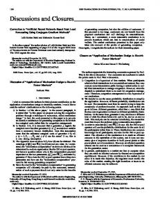
Fig. 2. Block structure of reduced system with nonlinearities.

Note that and in other words, the input to (55) is of size . For Krylov-based reduction, (55) can be reframed in blockmatrix terms as

(50) We observe that the reduction process consists simply of: 1) projecting the size- input subspace onto a size- subspace (50); 2) using this as input to a size- linear system (48) to and finally 3) representing obtain a size- state-space in the original size- state–space (50). (i.e., embedding) Equations (48)–(50) can be written in time-domain form as (51) with

(56) Equation (56) is a LTI system with inputs; it can, therefore, be reduced to a smaller system, using Arnoldi with multiple starting vectors. Let the reduced size be and the correspond; define , and let ing subspace be be the permutation matrix that reorders to produce for any vectors and . Similar to (56), (46) can be expressed as

(52) and (53) of the An approximation to any output original system can thus be obtained directly from the reduced where . state–space as We can now apply the concept of projection and embedding to the nonlinear reduction problem. Observe that an essential difficulty in reducing (45) is that, potentially, the direct product with itself is used as input. of the entire size- state space We can, however, reduce the dimensionality of this input by as the embedding in (53) from a -sized representing subspace. We then have

(54)

(57) inputs. This Equation (57) is a LTI system with system can, in turn, be reduced to a smaller one (of size ) using the Arnoldi method. The overall structure of the reduced system is shown in Fig. 2. We note that the effectiveness of size reduction is limited by the rapidly increasing sizes of the distortion input sources to the higher order Volterra systems. The actual input sizes, however, are determined by the numerical rank of the input coefficient matrices, e.g.,

Using (54), (45) becomes

(55) 2 We

thank Alper Demir for pointing out the advantages of Arnoldi over Lanczos in this context.

for (56). Owing to the fact that higher order derivatives of typical circuit functions are typically very sparse, this rank can be lower than the nominal size of the input space.

1280


B. Reducing Time-Varying Nonlinear Systems The procedure outlined in Section IV-A can be extended to nonlinear terms of a time-varying system. We start with (58) is a small input perturbation. To analyze perturbawhere tions conveniently, we now switch to the MPDE form of the differential equation (2)

(65) Equation (63) can be expressed in the operator form already encountered before in (7) (66)

(59) Let the unperturbed solution of (59) (with . Then, we can represent the perturbations to nonzero as

) be due

As discussed in Section III-B, (66) can be reduced using the Arnoldi method to the form (67) with

(60) Expanding the nonlinear functions series, we obtain

and

in Taylor

(68) and (69) and defined as

are as defined in Section III-B;

is

(70) (61) and represent the time-varying th Here, and respectively, evaluated derivative matrices of . Next, we express as with a small about can now be expressed scalar parameter. The solution in a Taylor series in

being the th block-row of , corresponding to the with th output harmonic or time point. as As in the time-invariant case, we approximate (71) Now, (64) becomes

(62) Substituting (62) in (61), and collecting the coefficients of etc., are powers of the following equations for obtained: (72) (63)

(64)

Equation (72) can now be expressed in block-matrix form as

(73)

(74)


Fig. 3. Low-pass filter

1281

!mixer!two bandpass filters.

Equation (73) has inputs; it can therefore be reduced to a smaller system using the techniques of Section III-B for and the corremultiple inputs. Let the reduced size be define . sponding Arnoldi subspace be Following a procedure similar to that for obtaining (73), (65) can also be expressed in matrix form as shown in (74). Equation (74), shown at the bottom of the previous page, is inputs, which can, in turn, be an LTV system with reduced to a smaller one (of size ) using the techniques of Section III-B. V. MACROMODELING CYCLOSTATIONARY NOISE

Equation (76) is structurally similar to (21) in [14], with replaced by the rectangular matrix . It is straightforward to apply the same reformulation steps as for LTI noise [14] to bring (76) to the form of (30), i.e., (77) TVP can now be applied to (77) to obtain a much smaller set of equations in the form of (36), which can be used to compute the noise contributions of the macromodeled system. VI. APPLICATIONS

When a system is macromodeled, it is also desirable to replace all its noise contributions by a few equivalent noise sources at the inputs or outputs.3 Usually, the power spectra of the equivalent sources have complicated frequencydependence, unlike those of the relatively simple white and flicker noise models typically used for internal noise generators. At the macromodel level, representing this frequency dependence perfectly requires computations with the original system, thus defeating the purpose of macromodeling. Instead, it is preferable to find approximate, but computationally inexpensive, forms of this frequency dependence. Such a capability has already been obtained for LTI systems with stationary noise [13], [14]. In this section, we sketch the extension to cyclostationary noise in LTV systems, useful for capturing phenomena such as frequency-translation and mixing of noise. The extension is achieved by applying the noise reformulation technique in [13], [14] to a block-matrix relation for cyclostationary noise [35] to obtain the form (30), and then applying TVP. We first recall the cyclostationary noise block-matrix relation [35]

(75)

OF

TVP

In this section, we present four applications of TVP. The first application is to a small idealized example, for the purpose of verifying TVP against hand calculations. The second application is to a switched capacitor integrator block. The third is to a RF mixer subsystem from the Lucent W2030 RFIC chip. The final application is to a dc/dc power conversion system. A. A Hand-Calculable Example Fig. 3 depicts an upconverter, consisting of a low-pass filter, an ideal mixer, and two bandpass filter stages. The component k values were chosen to be: nF, and nH. These values result in a low-pass filter with a pole at 100 kHz, and bandpass filters with a center frequency of 10 MHz and bandwidths of about 10 and 30 kHz, respectively. The LO frequency for the mixer was chosen to be 10 MHz. With reference to (17), the baseband-referred transfer funcand since they tions of interest in this case are appear in the desired up- and down-conversion paths. It can be hence, it suffices to consider shown that here. The expression for can be derived only easily using intuitive frequency-translation concepts; it is

where is the incidence matrix of the systems internal noise is a block matrix of HPSDs (harmonic power sources,4 is the spectral densities) from internal noise sources, and block matrix of noise HPSDs within the system, including the outputs. Analogous to (19) and without loss of generality, we can select the HPSDs at a single output by (78)

(76) 3 Input-

and output-referred noise sources are used extensively in circuit design. 4 Not to be confused with in (30).

A

Equation (78) is plotted for positive and negative frequencies in Fig. 4. Also plotted are the transfer functions obtained from and . It can be seen that for TVP TVP with the produces a reasonable approximation, whereas for

1282


(a)

(b)

Fig. 4. Simple circuit:

H1 (s) from TVP versus hand calculations. (a) 0ve frequencies. (b) +ve frequencies.

match is perfect, even though the original system is of order five. The poles of the original system and those from TVP are shown in Table I.

B. Switched Capacitor Integrator Block Our second application of TVP is to a lossy switchedcapacitor integrator block. The circuit was designed in a 0.35-

TABLE I

POLES (Hz)

OF

H1 (s), ORIGINAL AND REDUCED SYSTEMS


1283

The poles and residues of the system were obtained by eigendecomposition of the matrices, and used to construct expressions for the transfer function from the signal input to , this resulted in the the signal output envelope. For following analytical expression for the transfer function from the input to the output envelope:

(79)

Fig. 5. Steady-state output of a switched-capacitor integrator (with zero input).

CMOS process, and modeled using a Lucent MOS model (ASIM3) specifically intended for high-accuracy analog simulations. Comprising more than 150 MOS devices, it includes biasing, common mode feedback and slew-rate enhancement sections. The clock signal to the switched-capacitor filter had a time 12.8 MHz), but some period of 78 ns (i.e., frequency sections of the circuit operated at twice that frequency, i.e., 25.6 MHz. The steady-state waveform of the output node (in the absence of signal input) was obtained using shooting and is shown in Fig. 5. The output node did not have switching activity filtered out. Fig. 6 depicts a multi-time scale plot of the waveform at the output node in the presence of a 10-kHz sinusoidal input. (For details on how to interpret multi-time plots of waveforms, see [31] and [34]. The signal envelope (riding on the switching variations) is obtained directly from the waveform along a cross-section parallel to the signal time scale. By shifting the point of cross-section to along the clock time-scale, the signal envelope at different points of the clock waveform can be seen. Note how the (sinusoidal) signal is transmitted in the region between 60 and 78 ns on the clock time scale, but is cut out (because switches are off) between about 0–20 and 40–60 ns. For macromodeling, we chose to sample the output at 70 ns on the clock time scale, i.e., in the middle of the clock phase in which the signal is being transmitted. In other words, the transfer function being modeled is that between the input and the waveform obtained by taking a cross-section, parallel to the signal time scale, at 70 ns on the clock time scale in Fig. 6. A time-domain version of TVP was applied to reduce this transfer function. The macromodeling algorithm was run up to order 25. Fig. 7 depicts the input-to-output transfer functions from the full system ( marks), as well as from (dashed line) and two macromodels of size (solid line). As can be seen, even a tiny behavioral model of size 3 is sufficient to capture the response for input frequencies up to almost the switching frequency, while the size 25 model is accurate up to well beyond.

From the fact that the poles have negative real parts, it is seen that the system is stable. Further, we also observe that the smallest pole (168 kHz) has a much smaller residue than the one at 1.1 MHz. Such expressions can be useful to incorporate the precise characteristics of real circuit blocks into simple spreadsheet-type system design tools. Note that this is a LTI macromodel that abstracts the underlying continuous filter from the switching. If detail about the effects of switching is desired in the macromodel, all the timepoints along the clock cycle need to be incorporated as outputs to TVP. C. RF Buffer and Mixer Block A portion of the W2013 RFIC from Lucent Microelectronics, consisting of an I-channel buffer and mixer, was reduced nodes, and by TVP. The circuit consisted of about was excited by a local oscillator at 178 MHz driving the mixer, while the RF input was fed into the I-channel buffer. The time-varying system was obtained around a steady state of the harmonics circuit at the oscillator frequency; a total of were considered for the time-variation. , the upconversion Fig. 8 shows frequency plots of transfer function. The points marked “ ” were obtained by direct computation of (17), while the lines were computed and , using the TVP-reduced models with , a size reduction of two orders of respectively. Even with magnitude, the reduced model provides a good match up to the LO frequency. When the order of approximation is increased to ten, the reduced model is identical up to well beyond the LO frequency. Evaluating the reduced models was more than three orders of magnitude faster than evaluating the transfer function of the original system. easily calcuThe poles of the reduced models for lated on account of their small size, are shown in Table II. These are useful in design because they constitute excellent approximations of the full system’s poles, which are difficult to determine otherwise. D. PWM DC/DC Converter Our final application of TVP is to a boost-type dc/dc converter, featuring PWM feedback for output voltage stabilization. A simplified diagram of the circuit is shown in Fig. 9. When the switch closes, the inductor current rises linearly until the switch opens, after which the current is diverted through the diode into the load resistor. The peak current of the inductor is related to the amount of time the switch is

1284


Fig. 6. Multitime plot of switched-capacitor output.

TABLE II

POLES OF

Fig. 7. Frequency response of a switched-capacitor filter.

closed, i.e., the duty cycle of the switch control. This peak current determines the maximum output voltage, at node 3. The negative feedback loop operates by comparing the output voltage at node 3 with a reference to obtain an error voltage, which is used to control the duty cycle of the control to the switch. If the output voltage is lower than the reference, the duty cycle is increased, and vice versa. The nominal value of the input power source E was set at 1 V, while the reference voltage for the output was set to 1.4 V. The switching rate was 100 kHz. The resistance–capacitance (RC) pole formed at the load was at about 20 Hz. Initially, the loop gain including the PCM unit was set to ten. The steady state of the system was obtained with shooting

H1 (s) FOR THE I-CHANNEL BUFFER/MIXER

using about 100 timepoints. TVP (using time-domain steadystate matrices) was then run for ten steps. Fig. 10 shows plots of the transfer-function5 from the input source E to the regulated voltage at node 3. The marks were obtained from the full system, while the dashed and solid lines are from evaluations of the TVP-generated macromodels, as indicated. Observe that the size-4 macromodel is adequate to capture the system’s behavior up to the switching frequency. From the plots, we note that for low frequencies, the ripple rejection of the system is of the same order as the loop gain. The rejection, however, deteriorates significantly as the frequency rises; in fact, a small gain is seen at about 80 Hz. macroThe transfer function corresponding to the model (using poles and residues obtained by eigendecompo5 This is the 0th-harmonic transfer function, i.e., the average over the clock time scale.


1285

(a)

Fig. 8. I-channel mixer

H1 (s):

(b) reduced versus full system.

sition) is

small term (80) Note that the real parts of the poles are negative, indicating a stable system. To improve the supply rejection of the converter, the loop gain was increased to 1000, the steady-state recomputed using

shooting, and TVP macromodels generated again. The new transfer plots are shown in Fig. 11. Note that, as expected, the rejection at dc has improved to a factor of about 1000. However, the TVP-generated analytic transfer function (for ) is now

small term (81)

1286


unstable periodic solutions, because they solve boundary-value problems rather than initial-value (“transient”) problems. VII. CONCLUSION

Fig. 9. A dc/dc switching power converter with PWM feedback.

We have presented the TVP algorithm for reducing large LTV systems to much smaller ones with similar input–output transfer characteristics. The method is useful for automatic generation of accurate macromodels from SPICE-level descriptions, especially of communication system blocks. TVP has applications in system-level verification, producing analytical expressions for transfer functions, and intellectual property protection. We have illustrated TVP with several examples and obtained size reductions and computational speedups of orders of magnitude without loss of accuracy. We have also described extensions of TVP to incorporate signal path nonlinearities and for cyclostationary noise macromodeling. APPENDIX FLOQUET PARAMETERS AND LPTV TRANSFER FUNCTIONS

Fig. 10.

A dc/dc converter: transfer function for loop-gain 10.

It is well known that any LPTV system can be reduced to an LTI system and memoryless time-varying transformations. This result from Floquet theory (e.g., [10], [20]) implies that modes associated with it, the soany LPTV system has called Floquet parameters, corresponding to the eigenvalues of the underlying LTI system. In this section, we clarify the relationship between the Floquet parameters and the timevarying transfer function of the LPTV system. We start from the following ordinary differential equation description of a linear periodic time-varying system6 (82) (83) is periodic with period . Floquet theory [10], where [20] states that there exists a nonsingular -periodic matrix and a constant diagonal matrix such that (82) is equivalent to

(84) Hence, we obtain a system equivalent to (82) and (83)

Fig. 11.

A dc/dc converter: transfer function for loop-gain 1000.

(85) Note that the complex pole pair now has a positive real part, showing that the system is in fact unstable. The instability is generated by a combination of excessive phase shift and gain in the PWM feedback look. Using TVP-generated macromodels, numerical values of such unstable poles are easily obtained. Note that steady-state methods like shooting and harmonic balance, on which TVP relies, are indeed able to find

Equation (85) can be recognized to be an LTI system with the inputs and outputs multiplied by the periodic time-varying and . Since is diagonal, the equations quantities 6 The general case of LPTV DAEs can be addressed similarly using Floquet theory for DAEs [8].


are decoupled into modes. The entries of are the Floquet parameters. Following a procedure similar to that in Section III, the time-varying transfer function for (85) can be shown to be (86) Equation (86) can be solved explicitly, because is diagonal -periodic boundary and time-invariant. The solution with conditions can be shown to be

(87) and are the Fourier coefficients of and , where be . Then respectively. Let the diagonal elements of in (87) can be written as (88) and are the th elements of and where respectively. can have Equation (88) shows that for each , an infinite number of poles, which are simply the Floquet . Moreover, it is clear parameters shifted by multiples of that these poles are not time-varying. When (88) is put into (87), it is also evident that the residues of are, in fact, time varying. ACKNOWLEDGMENT The author would like to thank A. Demir for many fruitful discussions, particularly on nonlinear extensions of TVP. D. Long provided assistance and code for the frequency-domain implementation. T.-F. Fang and J. Thottuvelil pointed out the usefulness of TVP for switched-capacitor filters, power conversion circuits and IP protection. The author would also like to acknowledge the LTI model-reduction community in general, and his colleagues P. Feldmann and R. Freund in particular, for developing effective methods for modelreduction and establishing it as a useful tool for circuit analysis. REFERENCES [1] J. Aliaga, D. Boley, R. Freund, and V. Hernandez, “A Lanczos-type algorithm for multiple starting vectors,” Bell Labs, Murray Hill, NJ, Numerical Analysis no. 96-18, 1996. [2] D. L. Boley, “Krylov space methods on state-space control models,” IEEE Trans. Circuits Syst. II, vol. 13, pp. 733–758, June 1994. [3] H. G. Brachtendorf, G. Welsch, R. Laur, and A. Bunse-Gerstner, “Numerical steady state analysis of electronic circuits driven by multitone signals,” in Electrical Engineering. New York: Springer-Verlag, 1996, vol. 79, pp. 103–112. [4] M. Celik and A. C. Cangellaris, “Simulation of dispersive multiconductor transmission lines by Padé approximation by the Lanczos process,” IEEE Trans. Microwave Theory Tech., vol. 44, pp. 2525–2535, 1996. [5] , “Simulation of multiconductor transmission lines using Krylov subspace order-reduction techniques,” IEEE Trans. Computer-Aided Devices, vol. 16, pp. 485–496, 1997.

1287

[6] E. Chiprout and M. S. Nakhla, Asymptotic Waveform Evaluation. Norwell, MA: Kluwer, 1994. [7] L. O. Chua and P.-M. Lin, Computer-Aided Analysis of Electronic Circuits: Algorithms and Computational Techniques. Englewood Cliffs, NJ: Prentice-Hall, 1975. [8] A. Demir, “Floquet theory and nonlinear perturbation analysis for oscillators with differential-algebraic equations,” in Proc. ICCAD, 1998. [9] I. Elfadel and D. Ling, “A block rational Arnoldi algorithm for multipoint passive model-order reduction of multiport RLC networks,” in Proc. ICCAD, Nov. 1997, pp. 66–71. [10] M. Farkas, Periodic Motions. New York: Springer-Verlag, 1994. [11] P. Feldmann and R. Freund, “Efficient linear circuit analysis by Pade approximation via the Lanczos process,” IEEE Trans. Computer-Aided Design, vol. 14, pp. 639–649, May 1995. , “Reduced-order modeling of large linear subcircuits via a block [12] Lanczos algorithm,” in Proc. IEEE DAC, 1995, pp. 474–479. , “Circuit noise evaluation by Padé approximation based model[13] reduction techniques,” in Proc. ICCAD, Nov. 1997, pp. 132–138. [14] , “Circuit noise evaluation by Padé approximation based modelreduction techniques,” Bell Laboratories, Murray Hill, NJ, Tech. Rep. ITD-97-31678G, 1997. [15] P. Feldmann, R. C. Melville, and D. Long, “Efficient frequency domain analysis of large nonlinear analog circuits,” in Proc. IEEE CICC, May 1996, pp. 461–464. [16] R. Freund, “Reduced-order modeling techniques based on Krylov subspaces and their use in circuit simulation,” Bell Labs, Tech. Rep. 11273-980217-02TM, 1998. [17] R. Freund, G. H. Golub, and N. M. Nachtigal, “Iterative solution of linear systems,” Acta Numerica, pp. 57–100, 1991. [18] K. Gallivan, E. Grimme, and P. Van Dooren, “Asymptotic waveform evaluation via a lanczos method,” Appl. Math. Lett., vol. 7, pp. 75–80, 1994. [19] E. J. Grimme, “Krylov projection methods for model reduction,” Ph.D. dissertation, Elect. Eng. Dept., Univ. Illinois at Urbana-Champaign, 1997. [20] R. Grimshaw, Nonlinear Ordinary Differential Equations. Oxford, U.K.: Blackwell, 1990. [21] X. Huang, V. Raghavan, and R. A. Rohrer, “AWEsim: A program for the efficient analysis of linear(ized) circuits,” in Proc. ICCAD, Nov. 1990, pp. 534–537. [22] I. M. Jaimoukha, “A general minimal residual Krylov subspace method for large-scale model reduction,” IEEE Trans. Automat. Contr., vol. 42, pp. 1422–1427, 1997. [23] T. Lenahan, “Analysis of linear periodically time-varying (LPTV) systems,” Bell Laboratories, Tech. Rep. ITD-97-32813Q, Nov. 1997. [24] R. C. Melville, P. Feldmann, and J. Roychowdhury, “Efficient multitone distortion analysis of analog integrated circuits,” in Proc. IEEE CICC, pp. 241–244, May 1995. [25] S. Narayanan, “Transistor distortion analysis using volterra series representation,” Bell System Tech. J., May/June 1967. [26] A. Odabasioglu, M. Celik, and L. T. Pileggi, “PRIMA: Passive reducedorder interconnect macromodeling algorithm,” in Proc. ICCAD, Nov. 1997, pp. 58–65. [27] J. Phillips, “Model reduction of time-varying linear systems using approximate multipoint Krylov-subspace projectors,” in Proc. ICCAD, Nov. 1998, pp. [28] L. T. Pillage and R. A. Rohrer, “Asymptotic waveform evaluation for timing analysis,” IEEE Trans. Computer-Aided Design, vol. 9, pp. 352–366, Apr. 1990. [29] M. Rösch and K. J. Antreich, “Schnell stationäre simulation nichtlinearer ¨ vol. 46, no. 3, pp. 168–176, Schaltungen im Frequenzbereich,” AEU, 1992. [30] J. Roychowdhury, “A unifying formulation for analysing multi-rate circuits,” in Proc. NSF-IMA Workshop on Algorithmic Methods for Semiconductor Circuitry, 1997. , “Efficient methods for simulating highly nonlinear multi-rate [31] circuits,” in Proc. IEEE DAC, 1997. [32] , “MPDE methods for efficient analysis of wireless systems,” in Proc. IEEE CICC, 1998, pp. 451–454. [33] , “Reduced-order modeling of linear time-varying systems,” in Proc. ICCAD, 1998, pp. 53–61. [34] , “Analyzing circuits with widely-separated time scales using numerical PDE methods,” IEEE Trans. Circuits Syst. I, vol. 46, Sept. 1999. [35] J. Roychowdhury, D. Long, and P. Feldmann, “Cyclostationary noise analysis of large RF circuits with multitone excitations,” IEEE J. SolidState Circuits, vol. 33, pp. 324–336, Mar. 1998. [36] J. S. Roychowdhury, “SPICE3 Distortion analysis,” M.S. thesis, Elect. Eng. Comput. Sci. Dept., Univ. Calif. Berkeley, Elec. Res. Lab.,

1288


Memorandum no. UCB/ERL M89/48, Apr. 1989. [37] Y. Saad, Iterative Methods for Sparse Linear Systems. Boston, MA: PWS, 1996. [38] R. Telichevesky, K. Kundert, and J. White, “Efficient steady-state analysis based on matrix-free Krylov subspace methods,” in Proc. IEEE DAC, pp. 480–484, 1995. , “Efficient AC and noise analysis of two-tone RF circuits,” in [39] Proc. IEEE DAC, pp. 292–297, 1996. [40] V. Volterra, Theory of Functionals and of Integral and IntegroDifferential Equations. New York: Dover, 1959.

Jaijeet Roychowdhury received the B.Tech degree from IIT Kanpur in 1987, and the M.S. and Ph.D. degrees from the University of California at Berkeley in 1989 and 1993, all in electrical engineering. From 1993 to 1995, he was with the CAD Laboratory of AT&T Bell Labs, Allentown, PA. Since 1995, he has been with the Communications Research Division of Bell Labs, Murray Hill, NJ. His research interests include design and analysis of communication systems and circuits. Dr. Roychowdhury was awarded Distinguished Paper at ICCAD’91, and Best Papers at DAC’97, ASP-DAC’97, and ASP-DAC’99.