Reducing Field Failures in System Configurable Software: Cost-Based Prioritization Hema Srikanth IBM Software Group 4 Technology Park Drive Westford, MA srikanth
[email protected]
Myra B. Cohen Dept. of Comp. Sci & Eng. University of Nebraska-Lincoln Lincoln, NE
[email protected]
Abstract System testing of configurable software is an expensive and resource constrained process. Insufficient testing often leads to escaped faults in the field where failures impact customers and are costly to repair. Prior work has shown that it is possible to efficiently sample configurations for testing using combinatorial interaction testing, and to prioritize these configurations to increase the rate of early fault detection. The underlying assumption to date has been that there is no added complexity to configuring a system level environment over a user configurable one; i.e. the time required to setup and test each individual configuration is nominal. In this paper we examine prioritization of system configurable software driven not only by fault detection but also by the cost of configuration and setup time that moving between different configurations incurs. We present a case study on two releases of an enterprise software system using failures reported in the field. We examine the most effective prioritization technique and conclude that (1) using failure history of configurations can improve the early fault detection rate, but that (2) we must consider fault detection rate over time, not by the number of configurations tested. It is better to test related configurations which incur minimal setup time than to test fewer, more diverse configurations.
1. Introduction System configurability is a software development strategy that enables companies to develop and deploy software to a broad range of customers. The focus on system configurability rather than user configurability is characterized by the early binding time for the composition of components (or software environments) that are used for each instance of the system. In these types of systems a set of the environments must be installed, compiled and customized for use; they are not controlled by software parameters that can be
Xiao Qu Dept. of Comp. Sci & Eng. University of Nebraska-Lincoln Lincoln, NE
[email protected]
dynamically (and at little execution or setup cost) changed. Instead there is a significant cost associated with composing a single instance of the product and this can impact software testing techniques. In fact, our experience has shown that the time to configure and set up an environment for testing is the largest differentiating factor in this type of testing. The environments we aim to utilize during testing are analogous to those used by customers in the field, so we must install and compile these before testing can occur. In practice the primary costs of testing configurations inhouse consists of two elements:(1) setup (preparation) cost and (2) running tests. Compared with setup, running tests is a relatively fixed cost once a system instance is installed and configured. Software environments may consist of different operating systems, databases, and network and/or security protocols, etc. They may also include configurable parameters set by the customer such as the specific fix pack of a database, the number of concurrent connections allowed, driver types, details of the customers clustered environment or specific database settings. In a system configurable development model, a core set of components are built, tested and then composed each as a unique instance from a potentially enormous set of configurations before delivering to a large customer base; the full configuration space of a system can be in the thousands or millions. While economical from the standpoint of software development, research has shown that configurable software from the system testing perspective should be viewed as a family of software systems and that different faults will be revealed when running the same set of test cases under differing configurations [13]. System testing (testing conducted on a complete, integrated system to evaluate the system compliance with its specified requirements [10]) is the last phase before a product is delivered for customer use and thus represents the last opportunity for verifying that the system functions correctly and as desired by customers [9]. Configuring and testing
multiple complete, integrated systems (including hardware, operating system, and cooperating and co-existing applications) that are representative of a subset of customer environments is time intensive and as the number of possible components (or environments) increases the possible set of unique instances of configurations that can be deployed multiplies exponentially. Compounding this problem, research has shown that a defect found in the field often costs 100 times as much to fix as one found during requirements [1]. Based on the experience of the first author of this paper, field failures are more expensive to fix because the field issues have to go through additional processes and workflow before they come to the development team to be reproduced locally and deployed back into the customer environment. Further, every escape of a failure into the field that is found by a customer has a negative impact on system quality since this is measured by the volume of field failures. Companies, however, are often faced with lack of time and resources, which limits their ability to effectively complete system testing efforts. Recent work on prioritization of configurations [13] suggests that we can explicitly order configurations for testing to improve the rate of early fault detection in resource constrained situations, but this research has focused to date only on early fault detection. In the types of software studied in this work, the configurations are set at runtime and require installation. This work has ignored an important aspect of testing the class of software we term system configurable software – the difference in cost between testing different configurations. As a test architect at IBM, the first author’s experience is that the preparation of a system testbed for these types of system configurations takes from two to five days to complete. This includes installing and configuring all software environments for an individual configuration. Test planning and preparation may consume over 50% of the total test time and the effort of running system tests. Our typical system test is run in a clustered environment with an application server that includes at least three component values from a set of configurations – a specific operating system, back end database integration and the lightweight directory access protocol (LDAP). The time to run tests should consider both the test runtime and the preparation time such as installation and configuration times before test execution. Testing two instances of a system consecutively will differ in total test time depending on how much new setup is required to change from one configuration to the next. There have been some recent advances in cost-based prioritization. Do et al. present an economic model to capture costs related to test case prioritization [5, 6] that include parameters such as the time to fix faults, the time to run tests and revenue incurred. These models, while comprehensive, do not explicitly focus on the configurations of a system,
but rather on test cases, and may be too fine-grained for the system configurable software test environment. In this paper, we re-visit prioritization of configurations from a cost-cognizant point of view. We examine not only the increased rate of fault detection that can be achieved, but balance this with the cost of test setup required each time a configuration is modified. Our intuition is that we should focus on the total cumulative testing time taken to find faults in a system rather than on the cumulative number of configurations tested. We analyze this tradeoff based on real data gathered from the analysis of reported field failures of a large legacy enterprise system across two releases over the course of more than two years. We demonstrate that identifying configurations that are failure prone, and prioritizing test execution based not only on fault detection but also on the cost of changing and completing setup of configurations, may improve field quality by increasing the faults found within a time budget and minimizing escapes to the field. The primary contributions we make are to present: • an industrial case study of the potential effect of configuration prioritization on two releases of a large enterprise software system. • an evaluation of an alternative view of system configuration prioritization; one that is setup cost-cognizant. The rest of this paper is organized as follows. Section 2 provides some background on regression testing configurable software. Section 3 discusses the tradeoffs in cost vs. fault detection and presents the techniques we have developed to study this. Section 4 describes our case study while Section 5 presents our results. Finally, in Section 6 we present related work and in Section 7 we present our conclusions and future work.
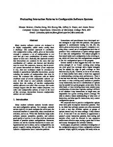
2. Background We begin with a small example to illustrate our problem domain and then present background on prioritization and combinatorial interaction testing. A model of our system is shown in Figure 1-A. Suppose we are testing an enterprise system that runs on three different operating systems, is supported on three different versions of Java™, and can be viewed using three different media players and web browsers. Each of these is considered a factor in our system. The individual options for each factor is termed a value. For instance the value Opera is one option for the factor Browser. We have a large set of system tests that we run to validate the system functionality. Running each system tests can take hours to complete. In order to test this system, we must first setup and configure the environment that consists of selecting one possible value from each of the four factors. Nine of the possible 81 configurations are shown in Figure 1-B. Research has shown (and our field experience
confirms) that if we run the same set of test cases using a different configuration different faults may be revealed [13]. Browser!
Java!
OS!
Player!
Opera!
JDK 1.3!
Mac OS X!
Quick Time!
Explorer!
JDK 1.4!
Windows XP!
Real Player!
Firebox!
JDK 1.5!
Linux !
Windows MP!
F1!
F2!
F3!
F4!
F5!
C1!
0!
0!
0!
0!
0!
C2!
1!
0!
0!
0!
1!
C3!
0!
0!
1!
1!
1!
C4!
1!
1!
0!
0!
0!
(A) Configuration Model!
Browser!
Java!
OS!
Player!
Opera!
JDK 1.3!
Windows XP!
Real Player!
2!
Firefox!
JDK 1.4!
Linux!
Real Player!
3!
Explorer!
JDK 1.5!
Mac OS X!
Real Player!
4!
Opera!
JDK 1.5!
Linux!
Quick Time!
5!
Explorer!
JDK 1.4!
Windows XP!
Quick Time!
6!
Opera!
JDK 1.4!
Mac OS X!
Windows MP!
7!
Firefox!
JDK 1.3!
Mac OS X!
Quick Time!
8!
Explorer!
JDK 1.3!
Linux!
Windows MP!
9!
Firefox!
JDK 1.5!
Windows XP!
Windows MP!
1!
( C) Fault Matrix- first four configurations!
1." < C3, C4, C1, C2 >!
2.2
Combinatorial Interaction Testing
2." < C2, C4, C1, C3 >! (D) 2 possible prioritization orderings!
(B) 2-way CIT Sample!
Figure 1. Configuration Model
2.1
run on the first configuration of our sample (1-B), (Opera, JDK 1.3, Windows XP, Real Player) did not reveal any faults during testing, while the same test suite run on the third configuration revealed three. We show two possible prioritization orderings in Figure 1-D. The first one finds all faults after testing only two configurations, and the second finds only three faults after the same time; it requires all four configurations to uncover all five faults.
Configuration Prioritization
When software is modified, regression testing is performed. This involves testing of both the new features and retesting the original features to ensure that changes have not introduced new faults. Many methodologies have been developed that focus on increasing cost-effectiveness through test case selection and/or test case prioritization (ordering) [7, 16, 17]. We only discuss the latter in this work. Many test case prioritization techniques have been proposed (e.g., [8, 18, 17]). Different techniques use different types of information to determine order such as branch, function or requirements coverage [17, 18]. In a typical regression testing scenario, a base program, P is used to collect data for prioritization of program P 0 . The assumption is that information from earlier programs predicts the fault occurrence in their modified counterparts. Regression testing for system configurable software may include not only test case selection and prioritization but also configuration selection and configuration prioritization. In [13], sampling was used to select configurations for testing of user configurable systems and these configurations were prioritized. As in test case prioritization information from prior releases was used to inform and predict which configurations should be tested first in the next release. The results of this work show that the order of configurations can impact the fault detection rate when the same set of test cases are run under differing configurations. To prioritize a set of configurations we first create a fault matrix. We show a simple matrix for the first four configurations of our example in Figure 1-C. Each row represents a configuration and each column a fault in the system. A zero in a column means that the fault is not revealed after running all test cases on that configuration, while a one means that at least one test case reveals it. As we can see, the test suite
Before we can determine prioritization orderings we must select a set of configurations to test. In our configuration example we have 81 configurations that are supported. If it takes 4 hours to run each test suite, and we can run tests continually, completely testing this system will take almost 2 weeks. Since the size of the configuration space increases exponentially in the number of factors it quickly becomes necessary to sample the configuration space. We can randomly select configurations, but we do not have knowledge of what an appropriate sample size is, and we have no guarantee of consistency. Prior work has moved towards sampling techniques that select representative subsets of configurations to test for combinations or interactions of factors and their values [13, 20]. One such method, combinatorial interaction testing (CIT) was originally created to sample a program’s input space. CIT sampling models the configurable options for a software system (factors) and their associated settings (values) and combines these so that all t-way (t > 1) combinations of settings are tested together [3]. Here, t is called the strength of testing, and when t=2, we call this pairwise testing. Recent studies suggest that CIT may provide an effective way to sample configurations for testing [12, 13, 20]. CIT samples can be modeled as a covering array, denoted CA(N ; t, k, (v1 v2 ...vk )), which is is an N × k array Pk on v symbols, where v = i=1 vi , and where each column i (1 ≤ i ≤ k) contains only elements from a set Si of size vi and the rows of each N × t sub-array cover all t-tuples of values from the t columns at least once. We use a notation to describe these with superscripts to indicate the number of factors with a particular number of values. A pairwise covering array with five factors, three of which are binary and two of which have four values, is written as CA(N ; 2, 23 42 ). Figure 1-B, shows a 2-way CIT sample for our model; this is a CA(9; 2, 34 ). All pairs of values between factors are combined. For instance we see all pairs of values from Browser and Java as well as all pairs of values from Java and Player. We can increase the strength of our sampling by including all 3-way combinations of values between factors. This will require a sample size of 27.
3. Cost-Based Prioritization In order to prioritize the CIT samples we first collect relevant information to drive the ordering. In [13] we examined ways to order CIT samples based on block coverage of each configuration’s test suite using program P to prioritize P 0 . We also examined alternative methods such as fault based prioritization and specification based prioritization. In this section we will present techniques that can be used to prioritize program P 0 ; ones that are aimed at capturing important information for system configurability. We will also present the metrics that we will use to capture the cost benefit tradeoff between the cost of configuration setup and that of fault detection.
3.1. Modeling Costs Prior work on cost models for prioritization have included many factors such as the time to fix the fault, the time to run the test case, and if the fault escapes into the field where a failure will impact customers (i.e. fault severity) [5, 6, 7]. Additionally, others have examined timeconstrained environments [19]. At IBM we have a thorough testing environment and expect that all easy to find faults are already found during unit testing. The types of faults we find due to configuration testing will likely be critical faults that will be treated as high priority. Our assumption is that due to their high priority, sufficient resources will be allocated to subsume the time tradeoff of fixing them. Our experience also shows that system test faults are highly complex to find and expensive, since it involves several days effort to configure an environment before any system test defects can surface. In other words, the overriding variable for running our tests is the time to install and build a new configuration. Based on this, we focus on this factor as the true cost of testing each configuration. Although the time to run system tests should also be considered in an absolute cost sense, it is relatively constant across different configurations so we do not consider it here. In the system configuration prioritization problem we aim to maximize fault detection while minimizing the install and build cost within a given time budget.
3.2. Prioritization Techniques We next describe three prioritization techniques that we propose which are based on the fielded test history data. In system configuration testing, we do not have prior code coverage therefore we must use other heuristics to drive prioritization. We make the assumption that faults found in one version will be indicative of the configuration value combinations for faults in the next version; i.e. these are the most complex and therefore the riskiest configurations. This is consistent with fault-based test case prioritization [16].
3.2.1
Factor-Value Prioritization
Our first method for prioritization aims to isolate the values of factors that are involved in the largest number of fielded failures. We use a previously developed algorithm to generate prioritized CIT samples [2]. We have successfully used this algorithm for configuration prioritization in [13]. The algorithm generates a single configuration at a time, driven by the product of the weights of each pairwise set of values. It stops when all pairs of factor-values are included in the sample. The resulting sample is a biased covering array. It covers all 2-way combinations of factor-values, but it is biased in that the factor-values with the highest weights occur in the earlier configurations. To set weights for this algorithm, we analyze the fault detection of each value and base the weights on this. Suppose we are setting weights using the fault matrix in Figure 1-C. Since C2 detects two faults and C2 is composed of Firefox, JDK™1.4, Linux® and Real Player, we say that Firefox, JDK 1.4, Linux and Real Player contributes to revealing fault 1 and fault 5. Similarly, for C3 , Explorer, JDK 1.5, Mac and Real Player contributes to revealing fault 3, 4 and 5; for C4 , Opera, JDK 1.5, Linux and Quick Time contributes to revealing fault 1 and 2. We then calculate the contribution of each factor-value in a cumulative fashion. A value’s contribution to one particular fault will be counted only once, even if it appears in different configurations. From this point of view, Firefox reveals two faults (F1 , F5 ), JDK 1.5 reveals all five faults, etc. The weight is equal to the ratio of the contribution of each value to the cumulative contribution of the factor to which the value belongs. We next consider the importance of each factor. Some factors will have more faults associated with them than others. Once again we calculate this and determine the ratio of the faults for the entire system. The final weight for each value in the system is the product of the factor weight and the value weight. 3.2.2 Pairwise Prioritization In a configurable system, harder to find faults (and the ones that our system tests should focus on) are most likely caused by interacting value combinations. In Figure 1, F1 will only be detected by the pair (JDK 1.4 or 1.5, Linux), which means, if we change the value of the operating system or of the Java™version to something else, this fault will not be revealed even if all other values remain the same as in C2 and C4 . In essence, only the pairs contribute to revealing F1 ; not the individual values of C2 and C4 . Our pairwise method of prioritization uses this idea to set weights to pairs, rather than to each single value. It uses a modified fault-matrix that represents fault detection for pairs of values, rather than for the entire configuration.
We show the pseudocode for an algorithm (Algorithm 1) that performs this prioritization. Once again, the aim is to generate a CIT sample where all pairs are covered, but with more important pairs covered first. The algorithm begins by adding all pairs to the U ncoveredP airs set (Line 1). Next it loops through and generates each configuration as follows until all pairs are covered. First it selects the uncovered pair that has the highest weight. Next it enters a loop to complete the configuration (Line 4). All pairs that are consistent with the values already selected for this configuration are put into a candidate set. For instance if we have already selected the pair Linux, Real Player, then any pair which contains this operating system and media player is considered consistent. From this candidate set we select the pair that has the highest value and add it to our configuration (Line 6 and 7). When we have selected values for all factors in our configuration we update (Line 8) and add this to the configuration sample (Line 9). 1: 2: 3: 4: 5: 6: 7: 8: 9:
Initialize U ncoveredP airs while U ncoveredP airs 6= ∅ do selectedvalues ← values in highest weight pair while Configuration is not complete do candidate set ← all pairs that are consistent with selected values new values ← Select highest weight pair from candidate set selected values ← selected values + new values update U ncoveredP airs add configuration to sample Algorithm 1: Pairwise Prioritization
3.2.3 Cost-Based Prioritization The two techniques mentioned above are considered traditional prioritization techniques and assume that the cost is the same for running each configuration and switching between configurations. Our last technique aims to minimize the cost of switching configurations. We use the same base algorithm as the factor-value prioritization, but instead of considering fault detection to set the weights, we use configuration switching cost — the lower the cost, the higher the priority. There are two modifications we make to the original algorithm. First, when we prioritize based on fault detection, we set weights ahead of time. But in the cost-based algorithm, the cost of switching configurations is dependent on the prior configuration, which means, the weights change after each configuration is generated; we dynamically calculate the weights at the start of each configuration generation. Second, while minimizing the cost, we still want to maximize the fault detection as much as possible. We use tie breaking to incorporate this aspect of the generation. When we have more than one choice of values with an
equal weight to select, we choose the one which will yield the highest fault detection (based on the value weights); in the original algorithm, we randomly select one. 3.2.4 Unordered As a baseline technique we use an unordered CIT sample. In this technique we generate a pairwise configuration sample using simulated annealing [4]. The generation does not occur a single row at a time, but rather the entire sample is modified during generation, viewed as a series of transformations. Therefore we can expect no bias in the ordering of the configurations of the sample.
3.3. Evaluation Metrics A common way to evaluate the effectiveness of different prioritization techniques is to measure the area under the curve when we plot the proportion of configurations run on the x-axis and the proportion of fault detection of the sample on the y-axis [8]. This metric can range from 0 to 1 (representing a proportion of the total plot area). If faults are found early in the sample, the left part of the curve will be high resulting in a larger area. The metric we use for CIT samples is called the Normalized Average Percentage of Faults Detected (NAPFD) (see [14] for a more thorough explanation). If we examine Figure 3 on page 8 we see that the topmost line has the earliest fault detection and composes the largest area (.82). The NAPFD can be formalized as follows. p CF1 + CF2 + ... + CFm + N AP F D = p − m×n 2n We have n configurations and m faults. CFi represents the number of the configuration (when testing in prioritized order) in which Fault i is found and p is equal to the number of faults detected by the prioritized set of configurations suite divided by the number of faults detected in the full CIT sample. If a fault, i, is never detected we set CFi = 0. Given our example in Figure 1-D, suppose we run only 3 configurations, then n = 3 and m = 5. With the first configuration order C3 , C4 , C1 , faults 3, 4, 5 are detected by the first configuration, C3 , and faults 1,2 can be detected by C4 , so CF3 = CF4 = CF5 = 1 while CF1 = CF2 = 2, and the NAPFD is 0.7. Similarly, with the second configuration order, C2 , C4 , C1 , CF1 = CF5 = 1, CF2 = 2, and CF3 = CF4 = 0 since faults 3, 4 are not detected by these three configurations. The NAPFD value is 0.43. The NAPFD assumes that all faults have the same severity and configurations have the same cost. In [7], Elbaum et al. address this limitation and propose a metric, APFDc , which considers the differences in fault severity and cost of the test case. However, in the APFDc the area measured is still that of fault detection. We would instead like to measure the area of cost where the x-axis is the proportion of the cost (or time in our case) and the y-axis remains the proportion of faults detected. We have developed a new metric to
capture this area based on the NAPFD that we call NAPFDc where c indicates cost. cF1 + cF2 + ... + cFm p N AP F Dc = p − + m×n 2n In this formula there are m faults and n units of cost (or time). cFi stands for the number (or units) required to find Fault i (we use discrete units of time). As before, p is equal to the number of faults detected by the prioritized set of configurations divided by the number of faults detected in the full CIT sample and if a fault , i, is never detected we set cFi = 0.
4. Case Study In this section we describe our case study designed to examine the cost-benefits in testing system configurable software. We answer the following two research questions. RQ1: Can we effectively prioritize software environments for in-house testing using historical field failure data? RQ2: Is there a cost-benefit tradeoff for evaluating prioritization of system configurable software? We begin by describing our software subjects and then discuss our dependent, independent variables, metrics and experimental methodology.
4.1. Objects of Analysis For this study we have used two consecutive major releases of a legacy product that allows enterprise customers to manage and customize organizational content for users and groups across an organization.1 The product has over a million source LOC and has been in the market for several releases and multiple years. Hundreds of enterprise customers are using this product to manage content from a single point of access. A typical mini-release of this product extends to a year, while a major release spans up to three years. The product team is spread around the globe with teams in US, India, China and Europe. The development team is moving away from a waterfall type model to a more agile process model with iterations of four weeks in length. The product has to satisfy the enterprise level customer requirements and must meet the aggressive reliability and performance requirements. Additionally, the product must ensure coverage across all supported environments. The system chosen has many environmental options, but for this study we focus on three major ones which have traditionally been the most problematic in the field and mirrors where we would therefore focus testing. 1 For proprietary reasons we cannot release the name or specific modules of this system
4.2. Experimental Methodology 4.2.1 Data Collection During the course of more than two years field failures from both releases were recorded. All of these failures are considered high severity failures because they escaped in-house testing and were due to complex combinations of configurations. The combinations of factors at the root cause of these failures were also recorded. Faults were associated with a pair of factors. More than 150 faults were considered for version one. Fewer faults were found in the second version (approximately 1/3). From this information we developed two fault matrices. The first is a standard matrix and the second is a pairwise matrix that considers the fault detection for pairs of values. 4.2.2 Prioritization We use the first release to determine a prioritization weighting for the second release. We focus on three environments that were deemed to be the most important in faultproneness based on the failure reports and choose to focus test efforts on this portion of the configuration model. This methodology is in line with what would happen in practice. According to the fault reports the following environments contributed to almost all of the fielded failures: Operating System (O), Database (D) and Security Protocol (S). We determined this based on the fact, the majority of failures were reported only when specific values were used for one of these, and remained undetected otherwise. There are five operating systems, three databases and seven security protocols. For the factor-value prioritization method we summed all faults reported for a particular factor-value and calculated the percentages of each with respect to all faults to determine the importance for prioritization. (Faults can be associated with more than one factorvalue at a time so these are not unique faults). For the pairwise prioritization technique we calculated the faults associated with pairs of configurations that were most often associated with the fault. Table 1 shows the factor-value model along with the percentage of faults associated with each value for the first version. The bold rows show the totals for each factor. As can be seen the operating system was associated with 72% of the faults in this version, while security was associated with 16%. Within operating system, O1 has the highest fault percentage while O3 has the least.
4.3. Dependent and Independent Variables Our independent variables are the various prioritization models described in Section 3, factor-value, pairwise, costbased and unordered. For each technique we generate five samples of configurations and average the results. We use more than one sample for each technique to reduce the chance that a random choice made during the algorithm is causing the observed result rather than the technique itself.
Factor
Value
Operating System O1 O2 O3 O4 O5 Database D1 D2 D3 Security S1 S2 S3 S4 S5 S6 S7
Percent Faults 72.0 41.0 16.3 0.4 6.6 35.7 11.9 61.2 29.1 9.7 16.1 22.0 9.4 24.7 2.2 26.0 6.3 9.4
Table 1. Version 1 - Faults Recorded Pair O1, D1 O1, D2 O1, S1 O1, S2 O1, S3 O1, S4 O1, S5 O3, S3 O3, S5
Fault Percent 17.4 5.8 6.7 4.0 2.1 0.3 7.9 0.6 0.6
Pair O3, S7 O4, D1 O4, D2 O4, S1 O4, S2 O4, S6 O4, S3 O4, S5 O5, D1
Fault Percent 0.6 2.1 2.7 1.2 0.6 1.8 0.3 0.3 7.3
Pair O5, D2 O5, D3 O5, S1 O5, S2 O5, S3 O5, S4 O5, S5 O5, S6 O5, S7
Fault Percent 4.9 4.3 4.9 0.9 9.8 1.2 5.8 0.9 4.9
Table 2. Version 1 - Pairwise Fault Matrix
For the factor-value prioritization model we first multiplied each percentage (as a fraction) by the weight of the factor and then used this as our weight. For instance for O1, we use the weight 0.30 and for O2 the weight is 0.12. In this way, the operating system values become the most important, followed by the security and finally the database values. We then created a CIT sample which resulted in 35 configurations. The model is a CA(35; 51 31 71 ). For the pairwise prioritization we use the data from Table 2. This table shows the pairs of values that are attributed to a set of faults. The percentage is the percentage of total faults attributed to this pair. All pairs not shown are zero. For instance, O1 combined with D1 constitutes approximately 17 percent of the faults while O1 combined with D2 accounts for 5.8 percent of the faults. The prioritized CIT samples for the cost-based prioritization is larger (45 configurations) due to repetition of some pairs early on in the sample. For RQ1 we use the first two prioritization techniques described, factor-value, and pairwise and compare this with the unordered CIT sample. For RQ2 we compare a single prioritization technique, factor-value, against the cost-based prioritization technique based on the results of RQ1. We also include the unordered technique as a baseline. Our dependent variables for RQ1 are the faults that could have been detected based on the fault matrix from the second fault matrix, and the NAPFD described earlier. For RQ2 we consider time to change configurations and therefore examine the NAPFDc as well as analyze the cumulative fault detection that will occur within specific time intervals. We compare this with the NAPFD results.
4.3.1 Compile/Build Cost For each prioritization schedule we calculate the time to compile and build the system as follows. Based on our experience it takes an average of one day to install/setup a new operating system and one half day for either the database or security environment. The absolute time will vary slightly between testers. An operating system change requires that the testers re-install both the security and database configurations, therefore each time an environment is changed we add time to install and configure all three. Using 8 hours as the time for a single day, we associate 16 hours for an operating system change (this includes both security and database) and 4 hours for any changes to the database and/or security. Since the security and database have no dependencies the time is additive. Next we assume that the time to run all tests on each configuration is a constant and is dropped from our equation. If for example we begin with a configuration consisting of O1, D3 and S7 the cost is 16 hours. If we next test O1, D1 and S6 the cost is 8 hours with a cumulative cost of 24 hours. Had we selected O1, D3 and S6 the cost would be only 20 hours (4 for the re-configuration). Likewise if we change operating systems and run O2, D3 and S7 (or any other combination of database and security) the cost is 16 for a total of 32 hours. We use these costs to weight the cost-based prioritization and to measure the NAPFDc for each configuration sample.
4.4. Threats to Validity Despite our best efforts these experiments suffer from some threats to validity. We outline the most significant ones here. We use only two consecutive releases of a single subject for our study. The subject used however is a large, real, deployed system and the faults reported are actual customer faults found in the field. We wrote several programs to manipulate our data, however we have cross validated these by hand to reduce the likelihood of any errors. One of the authors of this paper analyzed the fault reports from the field to develop the fault matrices. Although this is a threat, the other authors were not involved in this process and the matrices were developed and fixed before any prioritization techniques were applied. We also conducted this study retrospectively so we cannot be sure that the faults would have been uncovered by our in-house test suites. There is some variance in the time taken to install and compile the configurations between different testers. In this study we used an average time to compensate for this variance. Finally, there are other metrics that we may have used, but we have chosen ones that we believe are relevant to the problem and useful for others faced with the same problems.
5. Results In this section we present the results of our study to answer our two research questions.
1.0
0.9
0.9
0.8
0.8
0.7 0.6 0.5 0.4
!"#$%&'(")*+,
0.3
-".&/.0+,
0.2
12%&3+&+3,
0.1
Fault Detection Rate
Fault Detection Rate
1.0
0.7
0.82
0.6
0.71
0.5
Factor-Value
0.4
Cost-Based
0.58
0.3
Unordered
0.2 0.1
0.0 1
2
3
4
5
6
7
8
9
0.0
10 11 12 13 14 15 16 17 18 19 20 21 22 23 24 25 26 27 28 29 30 31 32 33 34 35
Number of Configurations
0.0
0.1
0.2
0.3
0.4
0.5
0.6
0.7
0.8
0.9
1.0
Proportion of Configurations Run
Figure 2. Cumulative Fault Detection Cumulative Cost (weeks)
To answer RQ1 we look at both the average percentage of faults detected across the 5 samples for each technique (factor-value, pairwise and unordered) and and the NAPFD values. We examine these values at configuration intervals which mimics a scenario where time is exhausted before testing is complete [13]. We show data for a single configuration and then show increments of 5 configurations up to 35 which is the size of the full CIT sample. These are shown in Table 3. As can be seen the NAPFD is quite low for all techniques after one configuration (.04 -.15); less than 1/3 of the faults are found. But it is as high as .76 for pairwise after 25 configurations are run. At this point 94 percent of the faults are detected, but only 83 percent of the faults are detected in the unordered sample. The unordered technique finds over 50 percent of the faults after 15 configurations, but at this point both prioritization techniques already detect over 80 percent of the faults and have NAPFDs of .63 and .67 for factor-value and pairwise respectively. There does not seem to be a large difference between the factor-value and the pairwise prioritization techniques. We also examine the cumulative fault detection in Figure 2. In this figure the x-axis is the number of configurations tested and the y-axis is the cumulative fault detection as a ratio of the total fault detection. Once again it seems that both of the fault-based prioritization orders outperform the unordered, however both seem relatively close in their ability to increase early fault detection. RQ1: Summary We conclude from this data that we can effectively prioritize system configurations using the history of escaped faults for a subsequent version of our program. We do not draw any conclusions about which of the prioritization techniques is stronger. To answer RQ2 we show only a single prioritization technique from RQ1 to compare with the cost-based technique. We have chosen factor-value because it does not require a specialized fault matrix, but the data allows us to draw the same conclusions for RQ1 as from pairwise. We begin with an examination of the graph for the NAPFD. This is shown in Figure 3. As has already been illustrated in Table 3 the factor-value NAPFD is higher than the un-
Figure 3. NAPFD Comparison 14
Factor-Value Cost-Based Unordered
12 10 8 6 4 2 0 1
3
5
7
9
11 13 15 17 19 21 23 25 27 29 31 33 35 37 39 41 43 45
Number of Configurations
Figure 4. Cumulative Cost in Weeks ordered sample. The area is also greater than the cost-based technique indicating that the factor-value prioritization is better. However, we must examine this further to understand cost. A different view of the data shows the cumulative cost (Figure 4), In this graph we show increments of weeks on the y-axis and the number of configurations on the xaxis. We see that the lowest cost is found in the cost-based method which is not unexpected. However, we also see that this cost is lower even after the other samples have run all of their tests. The cost-based sample has 45 (instead of 35) configurations in its sample, yet it finished in less than 6 weeks time (the horizontal line). The other techniques complete only about 1/2 of their configurations after 6 weeks. In fact to run the full CIT samples for unordered or factorvalue takes between 10-12 weeks. If we take a different view, we can graph the fault detection (y-axis) against the time in weeks (x-axis). We show this view of our data as Figure 5. Now it becomes clear that the cost-based prioritization, although it has a much lower NAPFD, improves early fault detection if we consider time. In 2 weeks it finds almost 90% of the faults and it finds all faults and is finished testing all configurations after 6 weeks. The factor-value prioritization on the other hand has only found 56% of the faults. Given this result we next examine the NAPFDc to see if this new metric is a better way to analyze the cost versus configuration tradeoff. We look at the NAPFDc for different time budgets. Figure 6 shows the graph for two differ-
Number Configs 1 5 10 15 20 25 30 35
Unordered Avg. % Faults Avg. Detected NAPFD 8 0.04 21 0.14 34 0.20 52 0.29 72 0.37 83 0.45 89 0.52 100 0.58
Factor-Value Prioritization Avg. % Faults Avg. Detected NAPFD 29 0.15 56 0.42 75 0.55 81 0.63 96 0.69 98 0.75 99 0.79 100 0.82
Pairwise Prioritization Avg. % Faults Avg. Detected NAPFD 29 0.15 66 0.44 80 0.59 85 0.67 88 0.72 94 0.76 97 0.79 100 0.82
Table 3. Fault Detection by Technique
1.0 0.9
Fault Detection Rate
0.8 0.7 0.6 0.5 0.4
Factor-Value
0.3
Cost-Based
0.2
Unordered
0.1 0.0 0
2
4
6
8
10
12
14
Cumulative Cost (weeks)
Figure 5. Cumulative Fault Detection By Week
ent time periods, 6 weeks and 13 weeks. We have chosen 6 weeks because that is when the cost-based technique completes and 13 weeks to allow for the completion of all other techniques. As can be seen the NAPFDc for the cost-based technique is the highest for both graphs after some initial time period. For the first few percentage points of time, factor-value outperforms cost-based, but then at some point we see an inversion (around 30% for 6 weeks and 10% for 13 weeks). The factor-value prioritization is always better than the unordered samples. RQ2: Summary For this question we believe that the answer is yes. There is a cost-benefit tradeoff that should not be ignored if significant time is incurred in setting up and configuring individual environments for testing. This can be viewed by graphing faults vs. cost and through our new metric, the NAPFDc .
6. Related Work There has been a considerable body of literature on test case prioritization [5, 6, 7, 16, 17, 19]. We focus on a few related threads of work. Do et al. [5, 6] present an economic model of cost for prioritization and conduct empirical studies to to examine how different time constraints affect the performance of test case prioritization techniques. Their model considers multiple costs and benefits, including the cost of test setup, test execution, and revenue. In our
work, we also address different time constraints, but focus on configurations (not test cases) and measure only the cost of configuration setup. Walcott et al. [19] examine timeaware test case prioritization to find an ordering which will always run within a given time limit and will have the highest possible fault detection based. The work focuses on the test case rather than the configuration and it assumes that each test case costs the same to run. Yilmaz et al. [20] sample the configurations space with CIT techniques and conduct fault characterization on the results. Their work considers only a single version of a system and does not prioritize. In a related thread Robinson et al. [15] propose a technique to detect latent faults based on configuration changes. Configuration changes are mapped to the underlying code and tests are then selected or created that cover the impacted areas. This work only addresses configuration relevant faults in a single version of a system. Our own work on configuration prioritization [13] presents different prioritization techniques at the configuration level however it does not consider the cost variance of changing between different configurations. Kimoto et al. [11] compare two algorithms to generate CIT samples for configurations that minimize the change cost. Their work is similar to ours in that they consider the time to switch configurations. However, they only present algorithms for minimizing the sample size and evaluate them on synthetic data. They do not consider fault detection or compare with other prioritization techniques.
7. Conclusions and Future Work In this paper we have presented a case study on two versions of an enterprise software system. We have shown that we can prioritize the configurations based on prior fault history to improve early fault detection. We have also shown that the traditional view of configuration prioritization does not hold when dealing with system configurable software that has involved setup between each configuration. In fact we have shown that the time to install and configure configurations between consecutive system test runs must be considered when time is limited. By examining prioritization in this new light we see that the actual time to run the same
0.92
Factor-Value
0.9
Cost-Based
0.8
1.0 0.9
0.81
Fault Detection Rate
Fault Detection Rate
1.0
Unordered
0.7
0.69
0.6 0.5 0.4 0.3
0.30
0.2 0.1
0.85
0.8 0.7 0.6
0.6 0.5 0.4
Factor-Value
0.3
Cost-Based
0.2
Unordered
0.1
0.0 0.0
0.1
0.2
0.3
0.4
0.5
0.6
0.7
0.8
0.9
1.0
Proportion of Time
0.0 !"!#
!"$#
!"%#
!"&#
!"'#
!"(#
!")#
!"*#
!"+#
!",#
$"!#
Proportion of Time
Figure 6. NAPFDc : 6 Week (left) and 13 Week (right) Budget
numbers of configurations varies greatly depending on the order in which we run them. In future work we plan to apply this method to a newer release of the system to discover if this works in practice. We also plan to examine other costs of system testing and to apply this to other configurable systems.
Acknowledgments This work was supported by IBM and in part by the National Science Foundation through award CCF-0747009, by the Air Force Office of Scientific Research through award FA9550-09-1-0129 and the Defense Advanced Research Projects Agency, award HR0011-09-1-0031. We thank G. Rothermel for comments on a draft of this work. .
References [1] B. Boehm and V. Basili. Software defect reduction top 10 list. In IEEE Computer, pages 135–137, Jan. 2001. [2] R. Bryce and C. Colbourn. Prioritized interaction testing for pair-wise coverage with seeding and constraints. Journal of Information and Software Technology, 48(10):960–970, 2006. [3] D. M. Cohen, S. R. Dalal, M. L. Fredman, and G. C. Patton. The AETG system: an approach to testing based on combinatorial design. IEEE Transactions on Software Engineering, 23(7):437–444, 1997. [4] M. B. Cohen, C. J. Colbourn, P. B. Gibbons, and W. B. Mugridge. Constructing test suites for interaction testing. In International Conference on Software Engineering, pages 38–48, May 2003. [5] H. Do, S. Mirarab, L. Tahvildari, and G. Rothermel. An empirical study of the effect of time constraints on the costbenefits of regression testing. In ACM SIGSOFT Symposium on Foundations of Software Engineering, pages 71–82, Nov 2008. [6] H. Do and G. Rothermel. Using sensitivity analysis to create simplified economic models for regression testing. In International Symposium on Software Testing and Analysis, pages 51–62, Jul 2008. [7] S. Elbaum, A. Malishevsky, and G. Rothermel. Incorporating varng test costs and fault severities into test case prioritization. In International Conference on Software Engineering, pages 329–338, May 2001.
[8] S. Elbaum, A. G. Malishevsky, and G. Rothermel. Test case prioritization: A family of empirical studies. IEEE Transactions on Software Engineering, 28(2):159–182, Feb 2002. [9] D. E. House and W. F. Newman. Testing large software products. SIGSOFT Software Engineering Notes, 14(2):71– 77, 1989. [10] IEEE. IEEE, Standard 610.12-1990,IEEE Standard Glossary of Software Engineering Terminology. 1990. [11] S. Kimoto, T. Tsuchiya, and T. Kikuno. Pairwise testing in the presence of configuration change cost. In International Conference on Secure System Integration and Reliability Improvement, pages 32–38, 2008. [12] D. Kuhn, D. R. Wallace, and A. M. Gallo. Software fault interactions and implications for software testing. IEEE Transactions on Software Engineering, 30(6):418–421, 2004. [13] X. Qu, M. B. Cohen, and G. Rothermel. Configurationaware regression testing: An empirical study of sampling and prioritization. In International Symposium on Software Testing and Analysis, pages 75–85, Jul 2008. [14] X. Qu, M. B. Cohen, and K. M. Woolf. Combinatorial interaction regression testing: A study of test case generation and prioritization. In International Conference on Software Maintenance, pages 255–264, Oct 2007. [15] B. Robinson and L. White. Testing of user-configurable software systems using firewalls. In International Symposium on Software Reliability Engineering, pages 177–186, Nov. 2008. [16] G. Rothermel and M. J. Harrold. Analyzing regression test selection techniques. IEEE Transactions on Software Engineering, 22(8):529–551, Aug. 1996. [17] G. Rothermel, R. Untch, C. Chu, and M. J. Harrold. Prioritizing test cases for regression testing. IEEE Transactions on Software Engineering, 27(10):929–948, Oct. 2001. [18] H. Srikanth, L. Williams, and J. Osborne. System test case prioritization of new and regression test cases. In International Symposium on Empirical Software Engineering (ISESE), pages 63–73, 2005. [19] K. R. Walcott, M. L. Soffa, G. M. Kapfhammer, and R. S. Roos. Time-aware test suite prioritization. In International Symposium on Software Testing and Analysis, pages 1–11, Jul 2006. [20] C. Yilmaz, M. B. Cohen, and A. Porter. Covering arrays for efficient fault characterization in complex configuration spaces. IEEE Transactions on Software Engineering, 31(1):20–34, Jan. 2006.