These models specify reef geometry by two parameters. They can .... 3 that a 5 km grid does not even remotely resolve major features of these reefs. Even a much .... system (x,y), the full nonlinear depth-integrated equations of motion are: at ax. + ay ... breadth, 1-10 km); t ~ T ~ to -t ~ f-1 (104 s for semidiurnal tides). In Eq. (3) ...
Pergamon
Prog. Oceanog.Vol. 40. pp. 285-324. 1997 © 1998 ElsevierScienceLtd. All rightsreserved Printed in Great Britain 0079-6611/98 $32.00 Plh S0079-6611 (98)00006-8
Reef parameterisation schemes with applications to tidal modelling LANCE BODE1, LUCIANO B. MASON2 and JASON H. MIDDLETON3
1School of Computer Science, Mathematics and Physics, James Cook University, Townsville, 4811, Australia 2School of Engineering, James Cook University, Townsville, 4811, Australia -¢School of Mathematics, University of New South Wales, Sydney, 2052, Australia Abstract - A variety of analytical models is used to investigate the effects on tidal propagation of a barrier reef system. These models specify reef geometry by two parameters. They can accommodate cases where water flows over reefs, as well as through inter-reef gaps, and also incorporate quadratic bottom friction. Although based on a one-dimensional approach, adaptations of a solution by Huthnance are used to account for the additional blockage effects associated with two-dimensional flow patterns near reef barriers. The present work adopts the philosophy that only a numerical approach can cope with the wide variations in reef geometry that are encountered in areas such as the Great Barrier Reef (GBR) region of Australia. Moreover, since typical model grids cannot resolve inter-reef gaps and other features with sufficient accuracy, a parameterised approach is needed to accommodate the conflicting demands of reef geometry and an economically feasible model resolution. The formulation of the analytical models is such that they can be applied immediately to standard numerical algorithms. Numerical experiments for flow in a channel, with a reef barrier across its centre, are used to test the parameterisation schemes. Comparison of the results for parameterised reefs with those obtained using extremely fine grids, shows convincing evidence of the success of the schemes. A separate method for automatically generating reef parameters has simplified the task of applying the methodology to real reefal systems. A tidal model of the Southern GBR, a region which exhibits unusual tidal behaviour, but which also has ample field data available for model testing, is used to demonstrate the accuracy that can be attained with the parameterised approach. Although tides are considered specifically in the present work, the formulation should be applicable with equal ease to the many other significant classes of low frequency motions in the GBR. © 1998 Elsevier Science Ltd. All rights reserved
1. INTRODUCTION T h e m a i n p u r p o s e o f this w o r k is to d e s c r i b e , test a n d a p p l y a p a r a m e t e r i s a t i o n s c h e m e that a l l o w s the u s u a l l y s u b - g r i d - s c a l e details o f coral reefs to b e i n c o r p o r a t e d into n u m e r i c a l l o n g w a v e m o d e l s in a d y n a m i c a l l y c o n s i s t e n t m a n n e r . R e e f s c a n e x e r t a c o n s i d e r a b l e effect o n the tides a n d o t h e r l a r g e - s c a l e flows in c e r t a i n parts o f the G r e a t B a r r i e r R e e f r e g i o n ( G B R ) . I m p o r t a n t q u e s t i o n s o f b i o l o g i c a l i n t e r e s t in t h e G B R , p a r t i c u l a r l y t h o s e r e g a r d i n g the a d v e c t i o n a n d d i s p e r s a l o f e g g s a n d larvae, c a n r e q u i r e n u m e r i c a l m o d e l l i n g at scales c o v e r i n g large port i o n s o f the c o n t i n e n t a l shelf, r a t h e r t h a n j u s t a r o u n d i n d i v i d u a l reefs (DIGHT et al., 1990). D e s p i t e the a d v e n t o f n u m e r i c a l t e c h n i q u e s s u c h as c u r v i l i n e a r c o o r d i n a t e s a n d finite e l e m e n t s , the e x t r e m e spatial c o m p l e x i t y o f the G B R r e e f m a t r i x h a s m e a n t that n o a p p r o a c h to m o d e l l i n g 285
286
LANCE BOOE et al.
the long wave equations can yet accommodate the conflicting requirements of high spatial resolution around reefs, and large areal coverage for regional dynamics. The GBR stretches for about 2000 km along the north-eastern continental shelf of Australia, from the waters of Papua New Guinea to south of the Tropic of Capricorn (9°S to 24°S), as shown in Fig. 1. More than 2500 reefs have been identified in this region, over which the reef
i"..': ,,~;;~. .~, ~
'-
"
..
CORAL SEA "'~
,
.
Southern GBR model domain
....
-.'r
t
| | r
t t
Fig. 1. Location map showing the extent of the Great Barrier Reef region, located between the coastline and the 200 m isobath (dashed line). The square sub-region, which is detailed in Fig. 2, is the Southern GBR model domain used in §8.
Reef parameterisation schemes with applications to tidal modelling
287
matrix exhibits a bewildering range of shapes and sizes. Despite its name, the GBR is in no way an unbroken chain of reefs. Although maximum lineal coverage can exceed 90% in places, this figure falls to less than 10% in other areas (IhCKARD et al., 1977). The so-called outer reef chain essentially occupies the edge of the continental shelf. Shoreward of the shelf break lie further reefs, often of considerable dimension. The GBR is separated from the coast by a relatively reef-free shelf area (the GBR "lagoon", where water is generally well-mixed vertically). More detailed descriptions of the physical structure of the GBR can be found in the reviews of MAXWELL (1968), PICKARD et al. (1977) and HOPLEY (1982). The extent to which the varying reef-forms modify the tidal response on the shelf is a matter of some interest. Given that the wavelength of barotropic tides is of order 1000 km, individual reefs should have little influence on overall tidal patterns. However, in the Southern section of the GBR, where pronounced semidiurnal amplification is observed, M]DDLETON et al. (1984) describe how the tidal characteristics of this area are modified considerably by the presence of reefs. It is now generally accepted that the overall tidal response in the Southern GBR (Fig. 2)
I
I
I
•
" ~"~;'"'~:~",,
~'
, ,,r-~
.
.
•
CORAL
.SEA
20 S
;,J :a ~.,
• "~
22 S
~
.::..-'2
-'..-g
;orn
and
;r Reefs
24 S 148 E
150 E
152 E
Fig. 2. Map of the Southern G B R region. All reef outlines are digitised from navigation charts. The square sub-region with an extent of 1° × 1° is shown in detail in Fig. 3.
288
LANCEBODEet al.
is consistent with the hypothesis first advanced in 1814 by the maritime explorer Flinders: that is, cross-shelf flow is inhibited by the massive reef coverage to such an extent that near-resonant conditions apply near the coast in the alongshore direction (although the overall shelf geometry of this region is also an integral component in the semidiurnal amplification process). A numerical tidal model of the Southern GBR is presented in this work, to demonstrate the capabilities of the reef parameterisation scheme. By contrast, in the neighbouring Central GBR, the coverage by reefs is so sparse that they can largely be ignored for tidal modelling purposes (ANDREWS and BODE, 1988). The parameterisation scheme is developed from a simple analytical, quasi-lD model, which describes flow through a chain of reefs and gaps. This theory is developed in §3 where impedance formulae are obtained for various reef configurations, using both linear and quadratic bottom friction. In §4, equivalent momentum equations are given for idealised reef elements, thus making the extension to time-dependent numerical modelling a relatively straightforward matter. Two-dimensional effects are incorporated in §5 by using results from HUTHNANCE (1985). Results from the various analytical reef models are summarised in §6. Numerical reef models are covered in §7, where the accuracy of the parameterisation schemes is demonstrated by comparison with results from high resolution, explicitly resolved, idealised reef geometries. The numerical scheme is applied to an M2 tidal model of the Southern GBR in §8, followed by overall conclusions in §9.
2. EXISTING APPROACHES TO REEF MODELLING The fundamental problem in adapting long wave models to shelf-scale reefal areas is one of spatial resolution, as is apparent from Fig. 3. This shows details of the square sub-region from Fig. 2, 1° × 1° in size, in which the reefs are overlain by a 5 km mesh. It is obvious from Fig. 3 that a 5 km grid does not even remotely resolve major features of these reefs. Even a much finer scale, e.g., the 1 nautical mile (nm) mesh used in the modelling of §8, fails to provide a sufficiently detailed explicit description of the reef matrix (1 nm = 1.8532 km). It is a clear over-simplification, therefore, to characterise individual grid squares in Fig. 3 as either 100% reef, or completely reef-free, the approach used in earlier shelf-scale numerical models of the GBR (SOBEY et al., 1977; BODE et al., 1981). Equally simplistic are analytical reef models, detailed below, which are forced to adopt idealised geometries, and hence are largely incapable of demonstrating anything other than the gross effects of reef structures on long wave propagation. Despite the simplifications adopted, previous analytical and numerical approaches have demonstrated the often significant effects of reefs on long wave dynamics, even though agreement with data is generally only qualitative. The present parameterised approach produces accurate shelf-scale solutions when tested against tidal data, as shown in §8, and in unpublished work which employs this methodology--BODE and MASON (1992, 1994a). 2.1. Analytical models
An early study by Church (personal communication) examined reef transparency in the Northern GBR, using two simple but diverse analytical treatments: a reefless shelf model with linear bottom friction; and a model in which the line of ribbon reefs is represented by an impermeable barrier at the shelf edge, thus forming an alongshore canal within the lagoon. Based on a comparison between model results and available data, particularly for phase differences, Church
Reef parameterisation schemes with applications to tidal modelling
I
0
-
., a
Hydrogral Passa
.
I
289
•
I
10
20 k m
w
•
,,f
a) II)
G
Fig. 3. Detailed map of reef outlines in the Hydrographer's Passage sub-region. The solid line indicates the navigational channel. A 5 km square grid is overlain for scale comparison purposes.
concluded that the almost unbroken line of ribbon reefs at the shelf edge forms a "barrier" that is largely permeable to tides. That is, the reefless model produces results much closer to reality for this region than the total flow barrier. HUTHNANCE (1985) undertook an extensive analytical treatment of reef porosity. This work uses two contrasting models of reefs with finite cross-shelf extent. In the first, reefs are treated as a wide unbroken region of shallow bathymetry over which all water passes. In this case, friction dominates the dynamics for reefs of significant cross-shelf width, resulting in a decoupling of the deep ocean and shelf domains, so that this solution approaches the total barrier case of Church above. A more realistic description is provided by the second model, in which ribbon reefs are represented as a chain of impermeable barriers, separated by channels. All the water passes through these inter-reef gaps. Here, Huthnance shows that the impedance to cross-shelf tidal flow can be attributed to two separate components. The first is a geometric constriction factor, caused by the fact that all water passing across the reef barrier is constrained to flow through the gaps. This part of the solution is ID in nature, and dominates the impedance for
290
LANCE BODEet al.
wide reefs. The pronounced 2D character of the flow at the entrance to and exit from inter-reef orifices introduces the second component of the impedance, the so-called "end effects", which dominate for reefs of thin cross-shelf extent. This impedance is shown to be equivalent to that obtained from a separate solution for a thin barrier (of zero cross-shelf width). The thin barrier solution is similar to that obtained by TucK (1980) for tidal flow across a continuous submerged reef. Huthnance concludes that unbroken reef chains produce such large frictional resistance that tidal communication between the ocean and the shelf must occur almost exclusively via the inter-reef channels. In accord with Church, he concludes that the geometry of typical reef structures is such that they are largely "transparent to tides". Although the broad thrust of that statement is largely consistent with observations, its simplicity tends to mask the extreme complexity, subtlety, and geographic variations in the GBR, and in the associated tidal response. Studies of tidal flow through large straits are presented by ROCHA and CLARKE (1987) who extend earlier results for sub-inertial flow by TOULANY and GARRETT (1984) tO arbitrary frequency. The flow through a single gap, designed to represent the Strait of Gibraltar, is obtained by solving the full wave diffraction problem in a rotating reference frame, utilising the solution of BUCHWALD (1971) for flow through a slit. The methodology is also extended to a finite number of orifices, to model tidal propagation through an island chain. In §3.1, we employ the scaling arguments of HUTHNANCE (1985) to show that the wave diffraction problem need not be treated for the smaller-scale tidal flows relevant to the GBR, and can be replaced by the solution to a simpler potential problem. A signifiCant contribution to the study of sub-grid-scale effects on tidal propagation can also be found in the Russian literature. The main theoretical results are summarised in KAGAN and KIVMAN (1993), who present a variety of parameterisation methods for islands and island chains. The parameterisation schemes are applied to a number of sensitivity studies on a coarse grid (5 °) global numerical M2 model. At this resolution, diffraction and Coriolis effects are essential contributors to the tidal response, as in ROCHA and CLARKE (1987). Importantly, KAGAN and KIVMAN (1993) show that parameterisation of island groups can significantly alter tidal patterns well away from their immediate vicinity, and can also lead to marked increases in energy dissipation rates in certain seas. 2.2. Numerical reef modelling
The stated motivation in HUTHNANCE (1985) was to obtain mathematical representations of reefs (i.e., parameterisations), that permit the incorporation of "a given reef system in largerarea models". Despite this, Huthnance concludes that analytical reef models are ultimately an impractical proposition for computing long wave dynamics, due to the GBR's inherent geometric complexity. The present work adopts the philosophy that only a numerical approach can accommodate the wide variations in reef geometry that are encountered in reality. Nevertheless, an essential step in the development of such numerical schemes is to test them against analytical or high accuracy numerical solutions using idealised geometries. An early attempt to incorporate reefs into numerical storm surge models of the GBR was made by SOBEY et al. (1977, 1982), whose finite difference (FD) treatment used the broadcrested weir method of REID and BODINE (1968). BODE et al. (1981) used this approach in an initial numerical study of the effects of reefs on tidal response in the Southern GBR. This model produced the observed semidiurnal tidal amplification of the area and gave approximate quantitative agreement with data, but was limited by the relatively coarse 5 nm spatial resolution. As demonstrated by Fig. 3, this is markedly larger than the dominant spatial scales of the reefs.
Reef parameterisation schemes with applications to tidal modelling
291
The need to use relatively coarse model grids, largely dictated by computer resources, provided the initial impetus for our parameterised approach. APELT and RICHTER (1985) treated reefs in the same region as impermeable barriers on an even coarser 20 km x 40 km FD grid, achieving reasonable qualitative agreement with the observed tidal pattern. If quantitatively accurate numerical solutions are required in the GBR, the early approach of using weirs or barriers on a "Yes/No" basis for coarse grids is inadequate. Adequate resolution of reefs requires a grid size As that is much smaller than that normally used in long wave models. Figure 3 suggests that a suitable As may need to be as small as a few hundred metres, i.e., around a tenth, or less, of conventional values. In explicit FD time stepping schemes, in which the maximum timestep At is governed by the stability criterion (At < As/~ghmax), total CPU requirements for 2D models vary as (As) -3. Costs vary as (As) -2 for implicit schemes. Clearly, if acceptable solutions can be obtained with an economical reef parameterisation scheme, the reductions in CPU requirements can be enormous. The aim of the parameterised approach is to provide acceptably accurate coarse grid solutions in areas of complex reef geometry, using a coding procedure to incorporate reef geometry as model data, in an efficient (and preferably automated) manner. Such a scheme should also be simple enough to require only minor modifications to existing numerical long wave models.
3. DEVELOPMENT OF REEF PARAMETERISATION SCHEME For completeness, and for use in the following analytical and numerical discussion, the 2D long wave equations are needed, in both full and simplified forms. In a horizontal Cartesian system (x,y), the full nonlinear depth-integrated equations of motion are:
at
ax
+ ay
at + ~ x an
at +
au
+ 03: av
+ay =°"
- jW= - gH ~xx
+fU=
- gHay
H2 U,
H2 V,
(1)
(2)
(3)
Here, t = time; "0 = ~(x, y, t) = sea-surface elevation, referred to Mean Sea Level (MSL) datum;
h = h(x, y) = undisturbed water depth; H = h + r/--- total water depth; f = Coriolis parameter; g = gravitational acceleration; U = (U,V) = horizontal transport per unit width, or depth-integrated velocity, defined by U = f~_hUdz=Hfi, where u = (u,v) is horizontal velocity and fi = (~,~) is its depth-average. Bottom stress is conventionally parameterised by a quadratic friction law, using the Colebrook-White formula for hydraulically rough boundaries, following SOBEY et al. (1982). This produces a weak dependence of the friction factor A on depth and bottom roughness. With a depth of h -- 30 m and a physical bottom roughness length of kh = 0.025 m, A = 1.73 x 10 -3. Shallower depths result in larger values---e.g., if h = 2 m, representative of water depths over reef fiats, A = 3.31 x 10 -3 for the same kb. Wind stress forcing at the sea surface is omitted, as only tidal motions are considered here. The linearised depth-integrated equations on an f-plane, in water of constant depth h, are
LANCE BODEet al.
292
~U 3t
fV=-
~1 gh 3x
rU h '
(4)
~V ~t + f U = -
~71 gh oy
rV h "
(5)
Eqs (4) and (5) are conventional linearisations of Eqs (1) and (2) under the assumptions that: nonlinear horizontal momentum advection can be ignored; total water depth H can be replaced by the ambient depth h in the pressure gradient term; and shelf bottom friction can be assumed linear, with coefficient r. The continuity Eq. (3) is unchanged. Linearisation of bottom stress involves replacing the term AIUI/H = lal by r. In the context of monochromatic 1D tidal flow with angular frequency o9, the result given in PROUDMAN(1953) can be used: 8
r = 37r )tUo ~- 0.85)tuo
(6)
where Uo is tidal velocity amplitude. This can be obtained by equating frictional dissipation over a tidal cycle for the quadratic and linear formulations, assuming a single, or at least a dominant constituent. PRANDLE (1978) discusses a range of such linearisations in one and two horizontal dimensions. More comprehensive treatments with applications to numerical modelling are given by SNYDER et al. (1979) and LE PROVOST et al. (1981). Note that for steady flow, the factor 8/37r reverts to unity, so that r = )tUo. With flows of the order of 1 knot ( ~ 0.5 m s - ' ), we obtain r ~ 10-3 m s-t from Eq. (6), typical of the values adopted in linear models of shelf dynamics. Assuming an e "°' time dependence for U, V and TI, in water of constant depth, U and V can be eliminated from Eqs (4) and (5) to yield the Helmholtz equation
32~ 32~1 Ox2 + ~y2 + K~T/= O.
(7)
The dispersion relation is
K~ -
o9(4 - f )
~rsgh~
,
(8)
and the complex frequency 0~ is given by 0"~ = o9[1 - irs(ogh~)-l].
(9)
Here, subscript "s" denotes the value of m r and h on the open (reefless) continental shelf.
3.1. Scale analysis for the GBR The aim here is to justify the use of certain key approximations for the GBR, and to compare the present formulation with other studies, notably ROCHA and CLARKE (1987). In particular, the question of wave diffraction is addressed. Following the approach used in §2 and §5 of
Reef parameterisation schemes with applications to tidal modelling
293
HUTHNANCE (1985), we scale variables as follows: r/ - Z (1 m); h, - / 4 o ( 3 0 - 5 0 m in interreef channels); (U,V) - U0 = Houo (with current magnitude, uo - l m s-~); (x,y) ~ L --~ d (reef breadth, 1 - 1 0 km); t ~ T ~ to-t ~ f-1 (104 s for semidiurnal tides). In Eq. (3), the scaled ratio of the terms r/, and V.U is (Z/T)/(Houo/L) = ZL/(HouoT) w, thereby producing the desired result of reducing end effects. For linear overflow reefs, ~rLR, defined in Eq. (24), is thus replaced by ~r'LR, and the ai in Eq. (24) are replaced by a'~, where O"LR----O'LR at" y(I)(W1)O" s
and
a'i = ai + 7qb(w,).
(47)
Although there are no firm theoretical grounds for this formulation, later comparisons with the results for highly-resolved reefs in the numerical experiments of §7 confirm its adequacy. A remaining minor defect is that end effects are still computed for the case of 100% reef (w---,0, b---*1). However, in the numerical model implementation, this situation is flagged, and the problem avoided by a separate treatment.
5.2. End effects for quadratic friction In this instance, no theoretical guidance is available, even for the quadratic barrier. For the linear barrier, end effects influence inertial and frictional terms equally, since ao in Eq. (35) is replaced by C~'o.By contrast, the quadratic momentum Eq. (41) contains C~o(which affects the linear inertial response), and/30 (which affects the quadratic friction coefficient, the magnitude of which is velocity dependent). An obvious approach is to consider end effects separately at the inertial and frictional limits, thereby isolating the effects on ao and /30, respectively. As friction becomes unimportant, the linear and quadratic momentum equations, Eq. (35) and Eq. (41), have the same form, depending only on C~o.This implies that for the QB case, ao in Eq. (41) should be replaced by C(o to incorporate end effects, as in Eq. (47). If we specify that /30 is replaced by /3'o =/3o + A/3o in Eq. (29) when incorporating end effects for the quadratic barrier, then from Eq. (41) at steady-state, /3'o is defined by
/3'°= K,U~o 3x
(48)
where Uo refers to the steady-state limit of the QB solution given in Eq. (33). With /3o given by Eq. (29),
304
LANCE BODEet aL
j hs
A/3o=/3'o - /30 = KsU~° 0x -
[
(l-b)
+
b]
w2 .
(49)
Given the dependence of/3'o on U~o, a numerical approach provides the most feasible method for determining A/3o. The numerical experiments, described later in §7, allow direct computation of Uo and hence/3'0 from Eq. (48). The relationship obtained empirically in §7.4 is (50)
A /3o = aw""/ O ( w ),
with a ~ 1.56 and n ~ - 0.56. In the case of quadratic overflow reefs, we replace w by w~, using the same heuristic arguments as above.
6. ANALYTICAL MODEL RESULTS The aim of this section is to explore the nature of the response to tidal forcing of idealised reef elements, by summarising the results of the previous analytical models for barriers and overflow reefs, with linear and quadratic bottom friction. The significance of including end effects is investigated, and an evaluation is also made of the quasi-steady approximations. In §4 we show that all linear models, except for the full reef case (LR) have the form OU a~ Ot -
07t gh, ox -
rsU aj h~
(51)
These models, when considered in harmonic form, yield an effective impedance, given by o" = aio) - iajrJh,. For the full reef (LR), o" is not available in this form, although it can still be found from Eqs (22) and (24). The corresponding momentum equation for quadratic friction is OU
O'q
~jK~IUIU"
(52)
Again, an effective impedance tr = a i t o - i/3jKslUI applies, with ]U[ given by Eq. (33), for all but the full reef case, QR. The (ai, aj) and (a~,/3j) combinations for specific models are given in Tables 1 and 2. Thus for all except the quadratic reef model which requires an iterative procedure, an explicit solution can be written down. Before covering the range of constricted flow solutions, we consider the basic properties of the open channel, for both linear and quadratic friction. To facilitate comparisons between linear and quadratic results, friction factors are tuned so that the steady-state velocities are approximately 0.5 m s-' for both models, with r~ = l0 -3 m s-j and A~ = 1.73 x 10⁻³ (§3). Figure 7 shows the amplitudes and phase lags for the unconstricted channel as a function of frequency, from steady-state to 4 cycles/day (cpd). Here amplitudes are normalised against respective steadystate transport: ULo, given in Eq. (14) for linear friction, and Ucm given by Eq. (34) for quadratic friction. For linear dynamics, Eq. (13) states that the response of the open channel is solely determined by the shelf impedance, trs, which depends on frequency and the relevant physical parameters. By contrast, the quadratic frequency response also depends on the magnitude of the applied
Reef parameterisation schemes with applications to tidal modelling
305
Open Channel Response
,0k o,,c_ w,s
I.
a-
1
°'t!
t
0.0
V2 0
1
2
0 3
4
Frequency(cpd) Fig. 7. Amplitude and phase lag in unconstricted channel, for linear (thin lines) and quadratic bottom friction (thick). Amplitude values are normalised by steady state values, ULo and Uoo; with quadratic friction, a discontinuity arises at zero frequency. Data from harmonic analysis of the linear and quadratic numerical experiments of §7 are indicated by " + " and " x ", respectively; circles ("o") denote maximum transports for quadratic friction.
forcing in the channel, so that increasing the pressure gradient, and hence the velocities, would make the response more frictional, and thus modify the shapes of the quadratic amplitude and phase curves in Fig. 7. Here, the two flow response extremes are: (i) frequency dominated (low friction or wavelike) where o- is real and the flow is in quadrature (90 ° phase lag) with the negative pressure gradient, -O~/ax; (ii) frictionally dominated (steady-state in the limit) for which cr is imaginary and the phase lag is zero. Note that when flow is frequency (frictionally) dominated, we call it "inertial" ("frictional"). As an example, the phase lag of U (arg(io~,.)) is approximately 76.5 ° at the M2 frequency for linear friction. In this instance, ~r,/o~ 2 ~ 1 - 0.24i, and flow is frequency dominated. Although the linear and quadratic models are tuned at steady-state, the decrease in velocity at higher frequencies reduces the relative contribution of friction to the value of ~r, thus making the quadratic response even more inertial. Also seen in Fig. 7 is the increase of quadratic amplitude response to values above 1.0, at low frequencies. The response returns abruptly to 1.0 at steady-state as the factor 8/37r in Eq. (6) reverts to unity. Fig. 7 shows marked variations in the frequency response of U for the open channel. To prevent these variations from masking the effects due to the constriction, it is desirable to remove the background open channel solution by computing the response relative to the unconstricted flow. For linear dynamics, the complex "constriction factor" ~ is defined as the ratio of U to the unconstricted value UL in Eq. (13). Using Eqs (12) and (16), ~ is given by = U = o',_= I~le -i(ae,~. U~. o"
(53)
306
LANCE BODE et al.
Table 1. Summary of linear analytical model formulations, including the incorporation of end effects (denoted by subscript "e" or a dash); the a~ and a'~ are defined in Eq. (39) and Eq. (47). Amplitude and phase of the constriction factor ~ at the M2 frequency are tabulated for geometries A, B1 and B2---see Fig. 8
Linear Model
ot~
~
[~1
A~
A (0.1,0.5) Open channel Barrier LB LBe Reef LR LRe QuasiLS steady LSe
1.0
1.0
I~1
~+
B1 (0.2,0.02)
I~1
A~
B2 (0.2,0.04)
Ctl
1.000 0.182 0.174 0.197 0.188 0.194
0.00 0.00 0.00 - 0.12 - 0.12 - 0.01
1.000 0.556 0.511 0.567 0.522 0.566
0.00 0.00 0.00 - 0.03 - 0.03 - 0.00
1.000 0.862 0.759 0.868 0.765 0.867
0.00 0.00 0.00 - 0.01 - 0.01 - 0.00
O/' 1
0.186
- 0.01
0.520
- 0.00
0.764
- 0.00
ao a'o
ao a'o
0/3 Ol' 3
1~1 is the relative amplitude response and Ath is the phase lag relative to the unconstricted flow. A similar definition applies for quadratic friction. As shown by Fig. 3, a grid resolution of 5 km can lead to a wide range of reef parameters w and b. Since ~ depends in general on geometry and frequency, results are presented in two distinct ways. Geometric effects are demonstrated by plotting contours of [~1 and Ark as functions of w and b at the M2 frequency. Variations with frequency are demonstrated by graphs of and A~b for the three specific geometries indicated on Fig. 8: A [(w,b) = (0.1,0.5)], B1 [(w,b) = (0.2,0.2)], and B2 [(w,b) = (0.2,0.04)]. B1 and B2 are used later in the numerical experiments of §7. For the linear barrier, ~La = l/a0 is real, so that AtkLB = 0. This means that the constriction factor, ~LB, is completely determined by geometry (i.e., by the values of w and b). Contour plots of ~LB in Fig. 8(a) show these variations with geometry. Numerical values of ~ at the M2 frequency are listed in Table 1 for geometries A, B1 and B2. The respective transports for these configurations are 18, 56 and 86% of the open channel value. Thus, when 80% of the channel cross-section is occupied by reef (B1 and B2), significant fluxes can still be driven by the applied pressure gradient. Figure 5 provides the explanation for this conclusion, by showing that readjustment of the pressure gradient will produce much higher velocities in the gap, thus compensating for the smaller cross-sectional area of the channel at the constriction. Only for the even more constricted geometry A is the transport significantly reduced. Table 2. Summary of quadratic analytical model formulations, including the incorporation of end effects (denoted by subscript "e" or a dash). Amplitude and phase of the constriction factor ~ at the M2 frequency are tabulated for geometries A, B1 and B2---see Fig. 10 Quadratic Model
ai
/3j
Open channel Barrier QB QBe Reef QR QRe QuasiQS steady QSe
1.0 oto ot'o
1.0 /30 /3'0
or3 t~'3
/31 fl'~
lull A~b A (0.1,0.5) 1.000 0.182 0.174 0.226 0.217 0.216 0.205
0.00 -1.60 -1.36 -12.45 -11.68 -2.17 -1.87
I~[ A& B1 (0.2,0.02) 1.000 0.555 0.510 0.583 0.537 0.582 0.535
0.00 -1.89 -1.60 -4.78 -4.32 -1.94 -1.65
lull A~b B2 (0.2,0.04) 1.000 0.861 0.758 0.873 0.771 0.874 0.772
0.00 -1.09 -1.13 -1.78 -1.76 -1.03 -1.07
Reef parameterisation schemes with applications to tidal modelling
'°1 F /
/
[
.///
/
7
°'1
/'
o.V, , / , b L
°"41
/" //
//
0.05
0,1
1.0
/// /I /
///// LB,,../'
/'
,
•
•
•
.
0.8 / O.6
// .6,' //
//
oo ~
///
307
1
//
// //
o.~
//
w
0.4
O.B
~ / /
0.2
//
O.S
(a)
0.0
1.0
0.0~
0.1
w
0.5
1,0
Fig. 8. (a) Constriction factors for the linear barrier, with and without end effects (LB, LBe), showing ~LB and I,,~Laelat the M2 frequency. A, BI and B2 denote geometries (w,b) = (0.1,0.5), (0.2,0.2) and (0.2,0.04), respectively. (b) Overflow reef solutions with end effects, showing contours of 191 for the linear reef (LRe) and its quasi-steady approximation (LSe).
When the barrier constriction extends along the full length of the channel (b = 1), a channel of reduced width, wAs, remains. Consequently, the transport is w times that of the open channel and ,~LB(W,1) = W, the minimum constriction factor for any w, as seen in Fig. 8(a). At the other extreme of b = 0, ~Ln(W,0) = 1, implying that any constriction completely disappears. This statement, that a narrow orifice presents no resistance to flow, is clearly unrealistic. It arises from the assumption of 1D solutions, and ignores the 2D nature of the flow in the neighbourhood of the gap--the end effects. These are demonstrated for the linear barrier by plotting contours of ~LBe = 1/% on the same figure. For geometry A, end effects reduce the transport from 18 to 17%; for B2, the change is from 86 to 76%. End effects can thus act to additionally restrict flow by a significant factor, particularly for thin barriers. In the limit as b---~0, end effects constitute the only restriction to flow. Fig. 9 shows the (constant) relative frequency response (LB) for B1 and B2, as well as the distinct contribution from end effects (LBe). Relaxing the barrier constraint that prevents flow over reef flats leads to the overflow reef solutions described in §3.3. On physical grounds, the larger cross-sectional area associated with this reef geometry leads to increased flows, and if friction were negligible, I~1 would increase in proportion to the cross-section. However, frictional effects are more pronounced across the shallow reef flat (hl = 2 m) than in the gap. Figure 9 shows that this results in a minimum at steady-state. Thus the overflow reef geometry not only allows more flow than the barrier, but the porosity increases with frequency, mirroring the accompanying effects of co on ~r. In §4, three quasi-steady solutions were introduced so that approximate momentum equations could be obtained for overflow reef cases. Testing of these was performed, in order to determine which most closely approximated the full reef solution. The first such model was excluded, as its response is independent of frequency. The second model produces the correct asymptotic behaviour at the steady-state and inertial limits, but differs significantly at mid-frequencies. Although still a compromise, the third model was chosen as its response is judged superior over the range of frequencies most likely encountered in long wave motions. Results for this linear quasi-steady model (LS) are given in Figs 8 and 9, and in Table 1. When the more realistic quadratic representation replaces linear bottom friction, we expect the overall response characteristics to remain similar. Figs 10 and 11 and Table 2 show that this is largely the case, although some subtle differences remain. Note again that the linear and
LANCE BODE et al.
308
0.65
(a)
'
'
(b)
Q,,;m,,t,y'B1
G m t r y B1
LB r LBe
LS, LEe 0.80
IFI
No End Effects
I/LS3 -2
LB
0.55
jl.~e
Wlth End Effects
-3 Lb 0.50
i
i
L
1
i
2 Frequency
i
i
3
o
i
,
L
1
2
3
(¢pd)
i
(clod)
Frequency
0.90 (C)
(d)
Geometry'B2 No End Effects
Geometry
LB t I.Be
B2
fLS3
LB 0.85
IFI -2 0.80
LRe
With End Efhlc~
0.75
i
i 1
i Frequency
i 2
i (clxI)
i 3
,
d'LS3e
-3 i
i 1
i Frequency
i 2
t
i 3
(clad)
Fig. 9. (a) Variation with frequency of linear solutions for J~l using geometry B1 [(w,b) = (0.2,0.2)], both with and without end effects: LB, LBe--barrier; LR, LRe--overflow reef; LS, LSe--quasi-steady solutions. (b) Corresponding Ark curves for geometry B1. (c) As in (a), but for geometry B2 [(w,b) = (0.2,0.04)]. (d) Corresponding A~ curves for geometry B2.
quadratic friction factors are tuned, so that a change in the applied forcing would alter the quadratic results. Figure 10(a) shows contours of I~QBI = [U/UQ], the magnitude of quadratic barrier (QB) constriction factor without end effects. Comparison with Fig. 8(a), and the values given in Tables 1 and 2, show that differences between I~QBI and ]~EBI are indeed minor, at the M2 frequency. Figure 11 shows, however, that the quadratic response differs significantly from the linear at low frequencies. The enhanced friction not only decreases the amplitude response, but also reduces the phase lag. Unlike the linear case, where relative phase lags are identically zero, the At~Qa values in Fig. 10(b) show a phase lag reduction, the magnitude of which increases as the gap fraction tends to zero. Physically, the larger velocities through the gap make the channel response more frictional, thus reducing the phase lag and amplitude. The constriction factor [ffQR[ for overflow reefs using geometry B2 is shown in Fig. 1 l(a), with corresponding plots of A~b in Fig. 1 l(b). As with the quadratic barrier, there are marked variations in I~l and A~b at low frequencies. At higher frequencies, the amplitude solutions correspond more closely to those for linear overflow reef dynamics. Values of A~b are similar to those for QB at low frequencies, but differ noticeably at the high frequency end. The increase in porosity of the quadratic reef over the quadratic barrier is greater than for the corresponding
Reef parameterisationschemes with applications to tidal modelling
,.o /
/,,. /,,,/ ,/,
/,,
77
0.5
o.,
/
I
0.8
--
,/'/,"7
s
// o~
1.0
/,, /,,,
//
os~.//"
,;~,4
Q,,
0.6
(,,, ,/,,
//0.. // ~, 0.5 / /;," / , , 0, ~'.. /(/ i,
0.4
~
0.05
0.1
-'
0.5
,-8
/)
/
'
1.5
0.05
,
0,4
W
IFI
//
o., ~ /
7/
/
O
#i~II
""
l
-2
0./ I
OA
Ic
5.0
!
0.1
0.5 W
-1 ~.5
i
o~~ ~ 0.05
1.O
0.5
0.1
o? / l i
0.5 t/0"1"
QRll
(b)
Z
0.5
W
/
t~
0.2
(,a) '
309
1.0
\\
\
ORe
\
QSe ~
o~
o
. 0,~
o
~
(d)
0,1
0.5
1.0
W
Fig. 10. (a) Constriction factor magnitude I~[ for the quadratic barrier, with and without end effects (QB,QBe), at the M2 frequency. A, B1 and B2 denote geometries (w,b) = (0.1,0.5), (0.2,0.2) and (0.2,0.IM), respectively. (b) Corresponding contours for A~b. (c) Contours of I~1 for the quadratic overflow reef solution with end effects (QRe) and its quasi-steady approximation (QSe), at the M2 frequency. (d) Corresponding contours for /t~b. linear cases. End effects again act to produce similar changes to those in the linear solutions, with flow rates reduced by approximately the same factors--see Fig. 11. The quadratic quasi-steady (QS) approximation provides a reasonable approximation to the quadratic reef solution (QR). Fig. 10(c) and (d) compare I~vl and A4b for the QRe and QSe solutions at the M2 frequency. Amplitudes for the quasi-steady solution generally compare well with those for the overflow reef. However, the pattern of the relative phase lags for QSe is closer to that of the quadratic barrier, shown in Fig. 10(b). Differences become marked as b---+l, where the reef solution is much more frictional. Amplitude and phase errors also increase with decreasing values of w. In reality, although very small values of w may be needed for some reef geometries, the resulting flow rates through such gaps will be insignificant, with the water tending to take other less restricted paths through the reef matrix. Therefore, any inaccuracies associated with using the quasi-steady reef solutions are expected to have minimal effects on overall flow patterns. It is instructive to consider the limiting values of ~v for all the above models, at the inertial (frictionless) and steady-state extremes. In the linear barrier and quasi-steady solutions, Eq, (51 ) shows that these limits are 1/~i and l/aj. For the overflow reef, Eqs (22) and (24) can be used to show that these limits a r e 1~or2 and l / s t. These values are all real, so that A& ~ 0 at the
310
LANCE BODE et al.
(a)
(b)
.. _~.~----~
0~0
QB
~J~
N~
-4
~
~ ~*QIIr~
IFI 0~o I
-8 0.40 ~
~
i i 1
i i
i
i 3
-12
i
i
i
L
1
(cpd)
Frequency
0.90
Geometry B1
B1 ( ~
i 2
i
2 Frequency
(c)
i
i
i
3
4
(cpd)
o.~-~-~_ QB
-4
0.80 °Se--
.. o_m-
--a
0.70
Geometry
0.60
i
i I
i
i 2
Frequency
i
i 3
Geometry B2
B2 i
-12
i
o
(cl)cl)
,
1
i
,
2 Frequency
i
i
3 (cpcl)
Fig. 11. (a) Variation with frequency of quadratic solutions for 191 using geometry B1 [(w,b) = (0.2,0.2)], both with and without end effects: QB, QBe--barrier; QR, QRe---overflow reef; QS, QSe---quasi-steady solutions. (b) Corresponding Aq5 curves for geometry B1. (c) As in (a), but for geometry B2 [(w,b) = (0.2,0.04)]. (d) Corresponding A~ curves for geometry B2.
two frequency limits--see Fig. 9. When end effects are included, the corresponding results are obtained by replacing the various c~ values by a ' . Similar analyses can be performed for the quadratic friction models, giving the respective limits of 1/c~i and 1/~-~fljfor the barrier and quasisteady models. In the QR case, these limiting values are 1/a2 and 1/~-~.
7. NUMERICAL REEF MODELLING
A prime aim in the analytical modelling described in the above sections is to allow a wider investigation than in HUTHNANCE (1985) of the effects of reef geometry on tidal response. In reality, however, a numerical approach is essential for accurate tidal modelling in view of the complexity of the GBR. The fact that equivalent momentum equations have been derived for reef modelling, and that the linear models can be extended to cover quadratic friction, makes the task of numerical model formulation a relatively simple exercise.
Reef parameterisation schemes with applications to tidal modelling
311
7.1. Model formulation In principle, Eqs ( 1 ) - ( 3 ) can be solved numerically by any one of a vast number of FD and finite element (FE) algorithms. In the present work we use the fully implicit two-dimensional FD model of BODE and MASON (1994b), adapted from that described by WILDERS et al. (1988). The equations are discretised on a standard, spatially staggered C-grid (MESINGER and ARAKAWA, 1976). Assuming for the present that nonlinear advective terms can be ignored, there are only relatively minor differences between Eq. (1) and the nonlinear quasi-steady Eq. (52): the nonlinear pressure gradient term is g/-/V-q is used in Eq. (1) rather than ghVB in Eq. (52); Coriolis accelerations, which are treated implicitly (BODE and MAsoN, 1994b), can be added as a body force; and the magnitude of the 2D transport, IUI = (U z + Vz) 1/2, replaces its 1D equivalent, ]UI. Thus, with w and b (and hence the relevant a and /3) known for a given grid square, any suitable numerical scheme can be applied to the modified momentum equations. Note that the use of the C-grid means that a different (w,b) pair in Fig. 6(a) applies for each of Eqs ( 1 ) (3), when treated numerically. With regard to the continuity equation, Eq. (3), Fig. 6(a) shows that in situations where the reef becomes exposed and thus acts as a total barrier, this equation must be replaced by b~ bU 3 v fl-(1-w)bl~t+~+~=0
(54)
or its numerical equivalent. In reality, reefs only tend to be exposed near the bottom of a spring tide, so that Eq. (3) will generally suffice, although it is simple to modify the numerical scheme to solve Eq. (54).
7.2. Numerical test bed Before applying the numerical schemes to the GBR, their performance is assessed by numerical experiments conducted in a suitable test bed. In all cases, the 2D (not the 1D) momentum equations are solved numerically. Both linear and quadratic models are tested. The respective friction parameters take the values adopted in §3, namely rs = 10-3 m s-~ and A~ = 1.73 x 10⁻³, with a larger value of As = 3.31 x 10⁻³ over reef flats of depth he. = 2 m. The standard test bed (Fig. 12) is a channel of length 25 nm, width 5 nm, and depth h~ = 30 m. The coarsest grid size, which is used for all the parameterised experiments, is Aso = 5 nm. The timestep used in all simulations is At -- 900 s. At its centre, the channel is constricted by a barrier. For the standard geometry used in most of the tests, the barrier covers 80% of the channel width (4 nm); the resulting gap is 1 nm wide and long. Each end of the channel is forced sinusoidally by a wave of amplitude 0.04 m, with the ends differing in phase by 180 °. Frequencies range from zero (steady-state) to 4 cpd, thus covering the full range likely to be relevant to continental shelfscale motions within the GBR. Steady-state velocities for the open channel are of order 0.5 m s~-L. At the coarsest resolution, the standard geometry of Fig. 12 has (w,b) = (0.2,0.2) for the central grid square. However, taking the 1:5 aspect ratio into account over the full length of the channel, (w,b) = (0.2,0.04). This corresponds to geometry defined as B2 in §6. In additional experiments, labelled B1, the obstruction extends along the length of the central grid square, giving (w,b) = (0.2, 0.2) for the channel as a whole. At grid resolutions other than Aso, the
312
LANCE BODE e t
al.
5 As0 I I I
G e o m e t r y B2
i
17 = - A e i ~ I I I I
A$o
=
| l
ASo
y!
I
15 45
I
q = A e i~ I I
I I
vJ I
Fig. 12. Test bed used in numerical experiments, with dimensions 25 nm long and 5 nm wide; harmonic forcing is applied at each end, as shown. The fundamental grid spacing used for the parameterised model is Aso = 5 nm. The B2 configuration of [(w,b) = (0.2,0.2)] for the central grid square is shown, along with successive levels of grid refinement used in the experiments ( A s o / A s = 5:1, 15:1, 25:1 and 45:1).
reefs and the gap are resolved explicitly. The values of As/Aso must be conformable with the C-grid; those chosen are 1/5, 1/15, 1/25 and 1/45, the sizes of which are displayed in Fig. 12. Note that with a grid spacing of Aso and parameterised reefs, the model runs approximately 2000 times faster for the implicit scheme used here than it does at the finest grid resolution. This factor would be around 105 with an explicit numerical scheme! Model results are compared by calculating the magnitude and phase of the total transport U across the central transect of the entire channel. Comparison with U for the open channel flow yields the relative amplitude and phase response, I,~l and Ath. As well as the barrier model, flow is also allowed over the obstruction, in order to test the various overflow reef schemes. 7.3. Numerical test results Numerical results from the parameterisation scheme using the coarsest grid size Aso, are compared with those obtained from the succession of increasingly finer-scale models that explicitly resolve the reef geometry of Fig. 12. Comparisons are also made with the analytical reef models described above. Given the large number of results obtained, only a selection is presented. Tables 3 and 4 summarise the LB and QB results for all grid sizes, using B2 geometry. These are also depicted in detail in Fig. 13. Results for the full range of experiments are presented in less detail in Figs 14 and 15: these show only the numerical results from the parameterised and finest grid (45:1 mesh ratio) models, along with the analytical solutions for BI, B2 and open channel geometries. Comparison with the analytical open channel solutions in Figs 14 and 15 shows that the numerical results exhibit small but finite errors. These figures give I~1 and A~b, the response relative to the absolute frequency response in Fig. 7, which shows both analytical and numerical results. On the scale of Fig. 7, differences between the analytical and numerical open channel results of Figs 14 and 15 are barely perceptible. Note also that relative errors are likely to be magnified at high frequencies, where amplitudes decrease markedly. In view of these numerical fluctuations, the frequency response is computed against the analytical open channel solutions for linear and quadratic friction, i.e., Eqs (13) and (34). The general pattern in the small numerical errors obtained with the open channel is seen in the results of all simulations (Figs 14 and 15). Nonlinearities cause an additional problem in
Reef parameterisation schemes with applications to tidal modelling
313
Table 3. Results of numerical test bed calculations for the total flow barrier with geometry B2 and linear friction. Entries show computed amplitude and phase of the constriction factor ~ as a function of forcing frequency and grid resolution, compared with analytical values, both with and without end effects Freq
(cpd)
0 0.25 11.5 0.75 I 2 4
LB
1
LBe
0.862 0.00 0.862 0.0 0.862 0.0 0.862 0.0 0.862 0.0 0.862 0.0 0.862 0.0
0,862 0.00 0.860 0.18 0.858 0.19 0.858 0.20 0.864 0.23 0.861 O. 18 0.879 0.22
0.759 0.00 0,759 0.0 0.759 0.0 0,759 0.0 0.759 0.0 0,759 0.0 0,759 0,0
Grid Resolution (As/As,) le 1/5 (I.759 0.00 0.757 0.18 0.756 0.20 0,756 0.21 0.761 0.24 0.760 0.20 0,778 0.25
0.785 0.00 0,782 0.20 0.778 0.32 0.776 0.37 0.778 0.26 0.782 0.08 0.801 0.42
1/15
1/25
1/45
0.776 0.00 0.772 0.20 0.769 0.32 0.767 0.37 0.768 0.26 0.773 0.08 0.793 0.42
0.770 0.00 0.767 0.20 0.766 0.32 0.766 O. 17 0.763 0.26 0.768 0.08 0.788 0.42
0.766 0.00 0.763 0.20 0.759 0.32 0.758 0.06 0.759 0.26 0.763 0.08 0.783 0.42
Table 4. Results of numerical test bed calculations for the total flow barrier with geometry B2 and quadratic friction. Entries show computed amplitude and phase of the constriction factor ,.% as a function of forcing frequency and grid resolution, compared with analytical values, both with and without end effects Freq
(cpd) QB
0 0.25 0,5 0.75 I 2 4
0.714 0.00 0.737 -5.63 0.792 -7.55 0.835 -5.72 0.851 -3.76 0.861 -1.02 0.862 -0.26
1 0.714 0.00 0.732 -3.23 0.783 -6.55 0.827 -5.30 0.847 -3.66 0.863 -1.14 0.884 -0.1 I
QBe 0.626 0.00 0,646 -5.76 0.696 -7.75 0.734 -5.89 0.749 -3.88 0.758 -1.05 0.759 --0.26
Grid Resolution (As/Aso) 1e 1/5 0,626 0,00 0,643 -3.38 0.690 -6.89 0.731 -5.71 0.749 -3.80 0.764 -1.05 0.783 -0.28
0.668 0.00 0.678 -2.51 0.722 -5.56 0.757 -4.48 0.773 -3.11 0.787 -0.99 0.809 -0.07
1/I 5
1/25
1/45
0.648 0.00 0.663 -2.98 0.708 -6.22 0.745 -5.05 0.770 -3.50 0.777 -1. I 1 0.799 -0.1 I
0.640 0.00 0.655 -3.13 0.701 -6.58 0.741 -5.48 0.756 -3.65 0.761 -1.40 0.794 -0.09
0.634 0.00 0.649 -3.25 0.695 -6.75 0.736 -5.64 0.752 -3.77 0.768 -1.22 0.790 -0.10
the a n a l y s i s a n d i n t e r p r e t a t i o n o f results for q u a d r a t i c friction. F i g u r e 16 s h o w s a t i m e series o f the c o m p u t e d v e l o c i t y n e a r the c h a n n e l c e n t r e for g e o m e t r y B2, at a f r e q u e n c y o f 0.25 cpd. T h e s t r o n g n o n l i n e a r i t i e s a n d r e s u l t a n t g e n e r a t i o n o f h a r m o n i c s are e v i d e n t in this trace. As a c o n s e q u e n c e , h a r m o n i c a n a l y s i s p r o d u c e s a m p l i t u d e s that are l a r g e r t h a n the m a x i m a at low f r e q u e n c i e s , as seen in Fig. 7. N u m e r i c a l l y - d e r i v e d a m p l i t u d e s closely f o l l o w the v a l u e s o b t a i n e d f r o m the q u a d r a t i c a n a l y t i c a l s o l u t i o n o f §3.3.2, a n d c a n e x c e e d the s t e a d y - s t a t e value. U n l i k e
314
LANCE BODE et al.
0.84 0.82
IFI
0.80
0
Parameterlsed
+
5:1
x i •
15:1 25:1 45:1
2
A¢
1 O:
0.78 t + + • +
+ -1
0.76 ~ - - ~ - ~ 0.74
[
0.80
IFI
-2
Linear
Linear
OI
+ x
..__---.---4
-2
0.75
0.70
0.65
F
-4 -6
0
1
-8
Quadratic
i
2
3
Frequency (cpd)
4
0
,
,
1
2
Quadratic
3
Frequency (cpd)
Fig. 13. Variation with frequency of numerical solutions for IU¢Iand A