Aug 6, 2009 - Anshul Agrawal, Thasia Madison, Lydia Tapia, and Nancy M. Amato. Parasol Lab, Dept. of Computer Science, Texas A&M University, College ...
Region Identification in Unsupervised Adaptive Strategy Framework Anshul Agrawal, Thasia Madison, Lydia Tapia, and Nancy M. Amato Parasol Lab, Dept. of Computer Science, Texas A&M University, College Station, TX 77843 {anshula, tmadison, ltapia, sthomas, amato}@cs.tamu.edu August 6, 2009 Unsupervised Adaptive Strategy(UAS) is a method which uses unsupervised learning techniques to perform adaptive motion planning in a given environment. The framework proposes automatic identification of regions. These regions divide the given environment such that they represent the planning space aptly based on the topological characteristics of the region. The current framework uses k-means clustering to perform region identification. In our modified approach, we first identify regions in the given environment using kmeans, hierarchical clustering and PG-means clustering individually. Next, we evaluate UAS’s performance by analyzing its results for improved efficiency and effectiveness due to the different regions identified by the three clustering techniques. We also examine how these regions affect the scalability of UAS to plan motions in complex environments involving cases where the workspace is not as easily mapped to the configuration space. Based on experimental results, we conclude the usefulness of each clustering method for the different motion planning environments.
“Region Identification in ...”, Anshul, Thasia et al., Texas A&M, August 2009
1
1
Introduction
The problem statement of motion planning (MP) is to figure out a path from the start location to the end location in a given configuration space. Even in a known environment, MP is not an easy problem to solve. There is strong evidence that any complete planner will have complexity that grows exponentially in the degrees of freedom of the robot [19]. Numerous randomized approaches have been proposed to solve this problem[11, 1, 4, 13, 18, 3]. The efficiency and effectiveness of these planners has been seen to be highly correlated with the planning space and the problem construction [7]. Adaptivity has been proposed as a solution [15, 17, 10, 5, 20, 2]. While significant improvement has been shown over non-adaptive approaches, these methods have all been seen to have serious drawbacks that limit their usefulness such as requiring significant user intervention (e.g., manual classifications of training instances for supervised machine learning methods, parameter tuning to set learning rates and learning weights) or restricting the types of problems they are able to solve. Unsupervised Adaptive strategy(UAS) for constructing Probabilistic Road Maps demonstrates a method which uses a combination of different adaptive learning strategies to make the motion planner more practical and efficient in complex environments with a variety of topological features. UAS explores a combination of two previously introduced adaptive methods, a feature-sensitive motion planning framework [15] and temporal adaptation (provided by the Hybrid PRM planner [10]). The UAS requires less user intervention, models the topology of the problem in a reasonable and efficient manner, can adapt the sampler depending on characteristics of the problem, and can easily accept new samplers as they become available. UAS uses the feature-sensitive framework to identify regions, except it replaces the tedious manual creation and labeling of training examples with unsupervised clustering. It then applies the adaptive strategy from Hybrid PRM in each of these semi-homogeneous regions. UAS assigns and adjusts sampler rewards based on the structural improvement the sampler makes to the roadmap [16]. The current implementation of this UAS framework uses k-means clustering to perform the unsupervised region identification. In this paper we compare and analyze two more clustering techniques namely hierarchical clustering and PG-means clustering individually with the framework. We create three versions of the UAS framework. Each of these versions runs one clustering method, that is, k-means, hierarchical, or PG-means [6]. We then execute the versions of UAS on several complex MP environments, where each environment poses a different challenge to the clustering strategy. We record the test-run results generated by each clustering technique and evaluate them against each other according to several criteria. We see if the generated clusters span over similar topology segments of the environment. We also test the regions for the runtime efficiency of the MP strategies on the regions generated to conclude if the regions are beneficial to UAS or not. At the end of the paper, we conclude the advantages and disadvantages of each clustering technique when integrated with the UAS framework, and suggest which one these three would be a better algorithm to use with the UAS.
2 2.1
Related Work Unsupervised Adaptive Strategy
UAS demonstrates how combining both the topology adaptation and sampler adaptation assists in answering the question of where and when to apply different sampling strategies. It simplifies the process of adaption that requires minimal user intervention, can be applied to any MP problem, and supports both topological and sampler adaptation. No previous method has all these characteristics. Augmenting an approach with topology adaptation enhances performance by focusing sampling in important or difficult regions of the problem. Adapting the sampler during the problem solution removes the burden of mapping samplers to region features and making sub-optimal choices. The results presented in this approach use workspace partitioning but can be easily extended to C-space partitioning as was done in [17]. In our method outlined in Algorithm 2.1, we first replace the requirement of manual training data creation and labeling with unsupervised learning for region identification. Next, we exchange the manual mapping of region types to samplers with the adaptive strategy provided in Hybrid PRM. This allows our method to continue to perform well as new sampling strategies are developed without requiring any additional input from the user. Also, the homogeneity of the region allows Hybrid PRM to quickly assess the space and
“Region Identification in ...”, Anshul, Thasia et al., Texas A&M, August 2009
2
select optimal samplers. This property reduces sensitivity to parameters such as learning rate and number of samplers. Finally, we use roadmap structure improvement metrics to automatically assign rewards/costs to the various samplers instead of tuning those parameters by hand, thus further eliminating parameter sensitivity. In the following subsections, we describe each step of the algorithm in more detail. Algorithm 2.1 Unsupervised Adaptation Method (UAS). Input. An environment E, a query Q, a set of samplers S, and an increment size m. Output. A roadmap R. 1: Identify (homogeneous) regions for planning in E. 2: Set P r(s) = 1/|S| for each sampler s ∈ S. 3: while Q not solved with R do 4: for all regions identified in E do 5: for i = 1 .. m do 6: Select sampler s according to probabilities P r. 7: Generate a sample with s and add it to R. 8: Update P r(s) according to the structural improvement of R. 9: end for 10: end for 11: end while 12: return R.
2.1.1
Feature Sensitive Motion Planning Framework
This approach was introduced as a method that used machine learning to characterize and partition a planning problem [15]. In this approach, the planning space is recursively subdivided until a machine learning method is able to classify a subdivision as appropriate for a planner from a given library. This topology mapping may be defined in either workspace or C-space. The strength of this method lies in its ability to identify a model of a problem’s topology that make certain regions appropriate for certain planners. However, other than recursive subdivision calls, it is not able to adapt planner applications over time. Another drawback of this approach is that it requires a mapping of samplers to regions, typically generated by machine learning techniques that require an “expert” to label hundreds of examples of training data. Such a mapping must be repeated as new planners are developed. 2.1.2
Hybrid PRM
Here, a reinforcement-learning approach provides sampler adaption by selecting a node generation method that is expected to be the most effective at the current time in the planning process [10]. Variations of this method that changed the learning process [21] and employed workspace information [12] have also been explored. The theory behind this method is that as the space becomes over-sampled by simple samplers, more complex samplers will be able to take over. However, these samplers are applied globally over the whole problem, and the features of the planning space, such as topology, are not used when deciding where to apply the selected method. Also, there are many parameters that need to be set for optimal application of the Hybrid PRM method such as initial sampler weights, sampler reward/cost assignment, how weights are adjusted during learning, and how long before beginning adaptation, to name a few. As new samplers become available, it is straightforward to add them to HybridPRM. 2.1.3
K-means Clustering
k-means, also referred to as the Lloyd’s Algorithm, is a clustering technique used to group n samples into k clusters in a given euclidean space until each observation belongs to the nearest mean. The initial k means are randomly selected in the given space. It then groups the observation samples with the closest means. Next, it finds the centroids to these regions and re-associates the samples with the different centroids based on the closest distance. The centroids of these clusters become the new means of the cluster. This process is repeated until convergence is achieved.
“Region Identification in ...”, Anshul, Thasia et al., Texas A&M, August 2009
2.1.4
3
Unsupervised Region Identification
To identify semi-homogeneous regions in the environment, UAS first constructs a small roadmap using each of the different samplers. Next, it partitions the nodes in the roadmap into c clusters using k-means clustering, for a given number of clusters c. There are many features that have been previously explored for region identification [15]. In the results shown in UAS, clustering is based on a set of features that are independent of robot type: visibility, X-position, Y-position, and Z-position. Then, it defines each region as the bounding box of each node set. Due to the use of positional values as features, clusters may result in overlapping regions. Choosing the number of clusters c is often difficult to perform using k-means clustering. In our motion planning application, the use of positional values (X, Y, Z) as features only complicates this selection because additional clusters will always provide an improvement. For example, consider the set of samples in Figure 1 for the Maze environment (Figure 4(a)). Partitioning the samples into 3 clusters (a) intuitively splits the environment into a single constrained region in the middle and two free regions on each end (samples are colored according to cluster membership). Increasing the number of clusters to 4 (b) begins to partition the already homogeneous regions. For example, the one circled region in (a) becomes the two circled regions in (b).
(a) 3 clusters
(b) 4 clusters
Figure 1: clustering based on a small roadmap in the Maze. In order P to overcome this limitation and automate the process, we examine the percentage of the variance k explained, ( i=1 σi2 )/σ 2 where σ 2 is the variance of the data set, for each c. Recall that the data set is defined by the features used for clustering (Section 2.1.4). We select the c that maximizes the second derivative of this function. This is commonly known as the elbow criterion [9, 14]. Intuitively, this criterion selects c such that adding additional clusters does not add sufficient information. In Figure 2, the average variance is plotted against the number of clusters for two environments, the L-tunnel and Maze. The “elbow” is indicated with a red star in each plot, and its calculation is shown in the inset. As noted above, the Maze is best represented by 3 clusters (see Figure 1(a)) instead of 4 (Figure 1(b)) which splits a region of homogeneous visibility. 2.1.5
Unsupervised Sampler Reward Assignment
Another area typically requiring user intervention is tuning the learning rate and the rewards/costs for each sampler. In addition, as new samplers are added to the set, these values may have to be adjusted. Similar to Hybrid PRM [10], UAS uses an exponential function to update sampler rewards. However, it defines the individual sample rewards differently. It rewards samplers on the range [0,1] as follows: cc-create and ccmerge nodes have a reward of 1 (since they always improve the roadmap) and all other nodes (e.g., cc-expand 2 and cc-oversample) have a reward of e−αvt , where vt is the visibility ratio of the node generated at time step t and α > 0. This gives nodes with low visibility a large reward and nodes with high visibility a small reward. The UAS found that α = 4 works well in practice because it weights the rewards on either end of the visibility spectrum (i.e., nearly 1 for the lowest visibilities and nearly 0 for the highest). It assigns equal weight to past performance and random selection when setting sampler probabilities.
4
“Region Identification in ...”, Anshul, Thasia et al., Texas A&M, August 2009
0.4
0.35
0.3
0.06 Elbow
0.25
0.08
0.3
0.025
Variance
Elbow
0.02 0.015
0.2 Variance
0.01 0.005
1
2
0.15
3 4 Clusters
5
0.04 0.02
0.25
0
1
2
0.2
3 4 Clusters
5
6
6
0.15
0.1
0.05
0.1
0.05 1
2
3
4
5 Clusters
6
7
8
9
10
(a) L-tunnel (elbow at 4 clusters)
1
2
3
4
5 Clusters
6
7
8
9
10
(b) Maze (elbow at 3 clusters)
Figure 2: Change in variance as the number of clusters increases.
3
Methods
In our approach to testing the two clustering techniques, we implemented a couple of Matlab scripts that run hierarchical clustering and PG-means clustering on a given data set and return the clusters formed by the respective methods. The UAS process is divided into three discrete steps. First, the UAS Framework samples a small number of points across the environment in the Configuration Space and calls these data points the training set. We modified the existing UAS Framework such that it outputs and stores the sampled training set data points into a file, which can be read by the clustering code. Then, the UAS program pauses for the user to confirm the generation of clusters. At this time, the user is expected to run the clustering methods, hierarchical clustering or PG-means clustering, on the data read in from the files containing the training set data. These Matlab script files perform the clustering specific operations and return the clusters in list form into another file as the output. At this point, the UAS program can be allowed to continue. In the final stage, the UAS program parses the file with the cluster outputs and performs Hybrid PRM on the different regions created to generate a roadmap that can solve a given query.
3.1
Hierarchical Clustering
Hierarchical clustering recursively groups the given set of nodes based on certain proximity distance metrics. We use binary agglomerative hierarchical clustering to perform a bottom-up recursive clustering of the two closest nodes at each step. There are three major conceptual steps involved in this process. Variance vs # of Clusters 0.09
1 0.9
0.08 0.02
0.8
0.06
Elbow
0.07 3.5
0.01
0.7
0
Variance
3
2.5
−0.01
0.04
2
0.03
1.5
0.02
1
0.01 0
0.5 6
10
3
8
1
(a)
9
4
5
2
7
0.6
0.05 0.5 1 2 3 4 5 6 7 8 9 101112131415 Number of Clusters
0.4 0.3 0.2 0.1
123456789111 012 13 14 15 16 17 18 19 20 21 22 23 24 25 26 27 28 29 30 31 32 33 34 35 36 37 38 39 40 41 42 43 44 45 46 47 48 49 50 51 52 53 54 55 56 57 58 59 60 61 62 63 64 65 66 67 68 69 70 71 72 73 74 75 76 77 78 79 80 81 82 83 84 85 86 87 88 89 90 91 92 93 94 95 96 97 98 99 100 Number of Clusters
(b)
0
0
0.1
0.2
0.3
0.4
0.5
0.6
0.7
0.8
0.9
1
(c)
Figure 3: A randomly generated 2D data set of 100 nodes (a) Dendrogram(with a maximum of 10 clusters/leaf-nodes) (b) Elbow Criterion (c) 3 Optimum Clusters • Distance Matrix: A distance array is first created as a list of all distances between each of the nodes in the input data set based on a certain distance metric in the configuration space. We chose this metric to be Euclidean distance, which is just the square-root of the sum of the squares of differences between two points.
“Region Identification in ...”, Anshul, Thasia et al., Texas A&M, August 2009
5
• Linkage Matrix: Next, a Linkage Matrix is created with ’Wards Distance’ as the linkage criteria. A Linkage Matrix is a connection analysis tool, that is used to represent the hierarchical clustering tree (see Figure 3.1(a)). The Wards Distance is the Inner squared Distance that can be used to minimize the variance of the clusters. • Optimal Clusters; In the last stage of creating clusters to represent the given environment, we apply the elbow criterion on the variance vs. number of clusters curve. The elbow criterion is used to find the optimal number of clusters by observing the rate of increase in the information gain rate with the increase in the number of clusters. (see Figure 3.1(b)). This criterion returns the number of optimal clusters k for the given environment, and we slice the hierarchical clustering tree at a height where there are only k leaf nodes. All the sampled nodes that lie in the sub-tree of these leaf-nodes fall under the same cluster.
3.2
Projected Gaussian-means Clustering
In the initial step, PG-means [6] generates a model of k clusters. The method used to learn the new model is called Expectation-Maximization (EM); however, any other method, i.e. k-means, can be used to obtain a new model. EM is a technique where the likelihood of generating an expected model of clusters is maximized based on logarithmic statistics. Once the best model of k clusters is obtained, the model and data set are projected to a 1-dimensional arbitrary axis to expedite the process of testing. After the projection phrase, the model is tested for its fitness with the data set. The Kolmogorov-Smirnov Test (KS-Test) is used to compare the model to the data set since it theoretically determines whether two given data sets differ significantly. At this time, the model may be accepted; if it is rejected, a new model is created using EM based on the previous learned model, and the PG-means process is repeated in this manner until a model is accepted. PG-means was set up with the following parameters and respective values: • Alpha: 0.001 • Number of projections: 12 • Data matrix: Sample nodes generated in the training phase of the UAS framework. The resulting information that the PG-means code provides is the number, location, and orientation of the final model of clusters. Finally, a Euclidean distance function was used to associate the nodes with their closest cluster centers.
4
Experiments
In this section, we compare the performance of our region identification methods within the UAS Framework. We study both rigid body problems and articulated linkages in environments of varying heterogeneity.
4.1
Experimental Setup
We implemented all planners using the C++ motion planning library developed by the Parasol Lab at Texas A&M University. RAPID [8] is used for collision detection computations. The hierarchical clustering was R clustering library. The PG-means library used for this research project performed using the MATLAB was provided by Greg Hamerly at Baylor University[6]. In our approach, connections are attempted between k “nearby” nodes according to a certain distance metric; here we use k = 20, C-space Euclidean distance, and a simple straight-line local planner. For a given region, we select a sampler based on the region’s average visibility. Our experiments map the regions as follows: in low visibility regions OBPRM is chosen, in medium visibility regions we use Gaussian sampling, and in high visibility regions uniform random sampling is used. Hybrid PRM is implemented as discussed in [10]. Sampler probabilities are initialized to the uniform distribution.
6
“Region Identification in ...”, Anshul, Thasia et al., Texas A&M, August 2009
(a) Maze
(b) L-Tunnel
(c) Hook
(d) Walls
Figure 4: Rigid body (a-c) and articulated linkage (d) environments studied. The robot must travel from one end to the opposite end. 4.1.1
Environments Studied
We explore several different rigid body and articulated linkage environments of varying topology, see Figure 4. In these environments, the witness queries have been designed to force the robot to traverse the entire problem space. This ensures that they capture the problem complexity. • Maze: This environment consists of two open areas connected by a maze of narrow tunnels. The tunnels vary from smaller than the robot (impassable) to just slightly wider than the robot. The robot is in the shape of a spinning top, and it is often very difficult for a planner to find feasible motions in the maze. • L-Tunnel: The L-shaped robot must rotate and translate in between three large obstacles to traverse an L-shaped maze. • Hook: The Hook environment has two walls with slits between them. The robot, a hook, must rotate and translate between the two slits to move from one side of the environment to the other. • Walls: The Walls environment has several chambers with small holes connecting them. Each chamber is either cluttered or free. The robot must traverse each chamber to solve the query. 4.1.2
Sampler Selection and Evaluation
To have a variety of sampling techniques in our available library of samplers, we have chosen samplers known to work well with varied amounts of obstacles. The samplers selected are: uniform random sampling [11], Gaussian sampling [4], and OBPRM [1]. For Gaussian sampling, we use two values of the Gaussian distance d: the robot’s minimum diameter, rd , and 2rd . We use the following metrics to evaluate planner performance: ability to solve a user-defined witness query, changes in types of nodes generated (e.g., cc-create, cc-merge, cc-expand, and cc-oversample), and collision detection calls as a measure of time.
4.2
Cluster Study
As demonstrated in [15], the training set (initial roadmap) must be cheap, fast, and represent the main features of the C-space. To define a good initial roadmap size, we chose to construct our small roadmap with fixed proportions of uniform random, Gaussian, and OBPRM nodes. Other sampling techniques could be used, but this set of planners mirrored the planners used for full map-building. We also used a low connection parameter (k = 5) to reduce cost. For example, roadmaps of 100 to 1000 nodes required from 48,664 to 400,848 CD calls. For the experiments here and those done in previous studies [15], low values of k capture the topology of the space. A larger value of k is used when maps are generated in the regions (Section 4.1.1). For each environment, the number of clusters identified by k-means and hierarchical clustering used the elbow criterion described in Section 2.1.4. PG-means used the KS Criterion to find this number.
“Region Identification in ...”, Anshul, Thasia et al., Texas A&M, August 2009
7
After the roadmaps were constructed, we studied the effect of the number of nodes on cluster quality. Recall that while all features, positional and visibility, are used in clustering, the positions are used to define region boundaries and visibility is used to define region homogeneity. For example, in the Maze environment, using k-means and hierarchical clustering, we found that with 200 nodes, 3 clear clusters were formed (Figure 1(a)). When the training set size was reduced to 100, three clear clusters were still able to be formed. Contrastingly, in the Maze environment using PG-means clustering, we found that with 200 nodes, 4 clear clusters were formed. However, when the training set size was reduced to 100, only two clear clusters were formed. For k-means, the visibility changes made two clear facts. First, an increased number of training samples increases the chance of finding clear, homogeneous regions. This was reflected in the difference in min/max ranges for different data set sizes. Second, while more samples are useful, they are not necessary to obtain good regions. This was made clear by the average visibility values, variance of visibility, and size and placement of the regions across all data set sizes. These results are shown in Table 1, where clusters are grouped by the relative positions of their members. Due to these facts, we chose a low, set number of samples (200) for clustering in the environments shown. However, as new problems are explored, the effects of sample size on cluster identification can be evaluated as shown. The results of hierarchical clustering, as illustrated in Table 2, were very similar to those of the k-means for the Maze environment. The number of clusters remained the same for different training set sizes. Also, the visibility ranges and the averages showed a very similar trend. There were three clusters identified, with one cluster being low visibility, and the others being high visibility. This could be attributed to the fact that both k-means and hierarchical clustering use the elbow criterion to determine the optimal clusters. Another reason for this would be that both of these clustering methods attempt to group nodes based on some representative value of the data; k-means uses centroids and hierarchical uses Wards distance. PG-means clustering shows an interesting trend with changing the number of nodes in the training data set. As evidenced by the results listed in Table 3, there is a drastic change in the number of clusters generated with changing the number of nodes. With 200 nodes, four optimum clusters were detected; however with 300 nodes, eleven optimum clusters were generated. This could be attributed to the KS-Test, which uses both the data set and the iterative cluster models it generates to learn and eventually conclude the optimal clusters. Thus changing the data set number makes a considerable impact on the resulting clusters. One way to look at the data is to look at the spread of visibility values as defined by the difference of the minimum and maximum visibility values in a cluster. In the PG-means tests, the spread varies with the number of nodes and clusters generated. For example, in the case of the 200 node training data set, two clusters have a medium spread (0.667,0.333) one has a wide spread (0.800), and one has a low spread (0.200). The magnitudes of the spreads also reflect the magnitudes of the standard deviation. In the 100 node data set, the spreads were the maximal values of 1.000 and 1.000. Additionally, in the 400 node data set, the spreads were distributed from 0.333 to 0.600 across the five clusters indicating little homogeneity in a single cluster’s visibility. Thus, the 200 node training data set was chosen for the purposes of our experiments.
4.3
Performance Study
In this section we compare the performance of k-means, hierarchical clustering and PG-means clustering, when they are integrated with the UAS Framework, in each environment. We allow the planner to attempt to solve the query with at most 5000 nodes for all environments except L-Tunnel in which we allow 8000 nodes. From our results displayed in Table 4, one can see that in the L-Tunnel environment, hierarchical clustering outperformed the other two clustering methods as illustrated by the low number of nodes generated and collision detection calls. However, no single clustering method dominates in every environment as evidenced by k-means’ strong performance in the Maze Environment. K-means not only generated the least number of nodes in this environment, it also made the least number of collision detections calls. Even though hierarchical clustering had to generate the largest number of nodes, it also had less collision detection calls than PG-means and k-means. This implies the topology was better captured by the clusters. In the final tested environment, the Walls environment, PG-means’ performance trumped the other two clustering methods’, which is supported by the extremely low number of nodes generated and resultant collision detection calls. Our results show that the number and placement of clusters is important to UAS’s ability to solve queries
8
“Region Identification in ...”, Anshul, Thasia et al., Texas A&M, August 2009 Cluster # 0
1
2
Data Set Size 100 200 300 400 100 200 300 400 100 200 300 400
Size (%) 27 18 20 21 42 43 48 47 31 40 32 31
Avg. 0.241 0.192 0.314 0.338 0.813 0.907 0.885 0.886 0.857 0.813 0.915 0.943
Visibility Std. Dev. Min 0.191 0.000 0.169 0.000 0.210 0.000 0.202 0.000 0.242 0.250 0.158 0.375 0.189 0.375 0.189 0.400 0.177 0.500 0.211 0.400 0.141 0.500 0.111 0.667
Max 0.600 0.500 0.667 0.667 1.000 1.000 1.000 1.000 1.000 1.000 1.000 1.000
Table 1: Cluster statistics on the Maze environment using different data set sizes. Clusters are grouped using k-means clustering. Cluster # 0
1
2
Data Set Size 100 200 300 400 100 200 300 400 100 200 300 400
Size (%) 23 14 25 17 45 41 26 34 32 45 48 49
Avg. 0.272 0.139 0.399 0.312 0.829 0.795 0.966 0.895 0.764 0.887 0.871 0.871
Visibility Std. Dev. Min 0.209 0.0 0.141 0.0 0.235 0.0 0.221 0.0 0.213 0.33 0.226 0.33 0.083 0.6 0.179 0.25 0.298 0.0 0.180 0.33 0.214 0.0 0.204 0.33
Max 0.6 0.5 0.8 0.75 1.0 1.0 1.0 1.0 1.0 1.0 1.0 1.0
Table 2: Cluster statistics on the Maze environment using different data set sizes. Clusters are grouped using hierarchical clustering. in a given environment. For instance, in the Maze environment, k-means and hierarchical clustering found three clusters and outperformed PG-means, which found four clusters. Furthermore, k-means performed slightly better than hierarchical clustering in the Maze environment and this could be attributed to the size and placement of the clusters k-means creates. In the Walls environment, PG-means generated three clusters as opposed to the six clusters that k-means and hierarchical clustering discovered. PG-means’ strong performance in the Walls environment demonstrates that the three clusters generated by PG-means were more appropriate for the Walls environment.
5
Conclusion
Using our feature evaluation techniques, we have been able to extract useful information about the environment which is consequential to more efficient motion planning. As a result of our research, we find that each clustering method has its strengths and weaknesses in a given environment. In the future we plan to use the information gathered to better choose a clustering method for a given environment. It is evident from the performance tests that improved clusters result in more efficient motion planning. Both the features used to
“Region Identification in ...”, Anshul, Thasia et al., Texas A&M, August 2009
9
define the clusters and the clustering techniques are useful in region identification. In future work, we intend to modify these features and test new features that define a configuration to study the resultant effect on this planning process.
6
Acknowledgments
We would like to acknowledge Greg Hamerly at Baylor University for providing the PG-means Matlab libraries.
References [1] N. M. Amato, O. B. Bayazit, L. K. Dale, C. V. Jones, and D. Vallejo. OBPRM: An obstacle-based PRM for 3D workspaces. In Robotics: The Algorithmic Perspective, pages 155–168, Natick, MA, 1998. A.K. Peters. Proc. Third Workshop on Algorithmic Foundations of Robotics (WAFR), Houston, TX, 1998. [2] J. Berg and M. Overmars. Using workspace information as a guid to non-uniform sampling in probabilistic roadmap planners. Int. J. Robot. Res., 24(12):1055–1072, 2005. [3] R. Bohlin and L. E. Kavraki. Path planning using Lazy PRM. In Proc. IEEE Int. Conf. Robot. Autom. (ICRA), pages 521–528, 2000. [4] V. Boor, M. H. Overmars, and A. F. van der Stappen. The Gaussian sampling strategy for probabilistic roadmap planners. In Proc. IEEE Int. Conf. Robot. Autom. (ICRA), volume 2, pages 1018–1023, May 1999. [5] B. Burns and O. Brock. Toward optimal configuration space sampling. In Proc. Robotics: Sci. Sys. (RSS), 2005. [6] Y. Feng and G. Hamerly. Pg-means: Learning the number of clusters in data. In Neural Information Processing Systems, pages 393–400, 2006. [7] R. Geraerts and M. H. Overmars. Reachablility-based analysis for probabilistic roadmap planners. Robotics and Autonomous Systems, 55:824–836, 2007. [8] S. Gottschalk, M. C. Lin, and D. Manocha. OBB-tree: A hierarchical structure for rapid interference detection. Comput. Graph., 30:171–180, 1996. Proc. SIGGRAPH ’96. [9] T. Hastie, R. Tibshirani, and J. Friedman. The Elements of Statistical Learning: Data Mining, Inference, and Prediction. Springer, 2001. [10] D. Hsu, G. S´ anchez-Ante, and Z. Sun. Hybrid PRM sampling with a cost-sensitive adaptive strategy. In Proc. IEEE Int. Conf. Robot. Autom. (ICRA), pages 3885–3891, 2005. ˇ [11] L. E. Kavraki, P. Svestka, J. C. Latombe, and M. H. Overmars. Probabilistic roadmaps for path planning in high-dimensional configuration spaces. IEEE Trans. Robot. Automat., 12(4):566–580, August 1996. [12] H. Kurniawati and D. Hsu. Workspace-based connectivity oracle - an adaptive sampling strategy for prm planning. In Algorithmic Foundation of Robotics VII, pages 35–51. Springer, Berlin/Heidelberg, 2008. book contains the proceedings of the International Workshop on the Algorithmic Foundations of Robotics (WAFR), New York City, 2006. [13] S. M. LaValle and J. J. Kuffner. Randomized kinodynamic planning. In Proc. IEEE Int. Conf. Robot. Autom. (ICRA), pages 473–479, 1999. [14] L. Lieu and N. Saito. Automated shapes discrimination in high dimensions. Proc. of SPIE, 6701 – Wavelets XII(67011W), 2007.
“Region Identification in ...”, Anshul, Thasia et al., Texas A&M, August 2009
10
[15] M. Morales, L. Tapia, R. Pearce, S. Rodriguez, and N. M. Amato. A machine learning approach for feature-sensitive motion planning. In Algorithmic Foundations of Robotics VI, pages 361–376. Springer, Berlin/Heidelberg, 2005. book contains the proceedings of the International Workshop on the Algorithmic Foundations of Robotics (WAFR), Utrecht/Zeist, The Netherlands, 2004. [16] M. A. Morales A., R. Pearce, and N. M. Amato. Metrics for analyzing the evolution of C-Space models. In Proc. IEEE Int. Conf. Robot. Autom. (ICRA), pages 1268–1273, May 2006. [17] M. A. Morales A., L. Tapia, R. Pearce, S. Rodriguez, and N. M. Amato. C-space subdivision and integration in feature-sensitive motion planning. In Proc. IEEE Int. Conf. Robot. Autom. (ICRA), pages 3114–3119, April 2005. [18] C. L. Nielsen and L. E. Kavraki. A two level fuzzy PRM for manipulation planning. Technical Report TR2000-365, Computer Science, Rice University, Houston, TX, 2000. [19] J. H. Reif. Complexity of the mover’s problem and generalizations. In Proc. 1EEE Symp. Foundations of Computer Science (FOCS), pages 421–427, San Juan, Puerto Rico, Oct. 1979. [20] S. Rodriguez, S. Thomas, R. Pearce, and N. M. Amato. (RESAMPL): A region-sensitive adaptive motion planner. In Algorithmic Foundation of Robotics VII, pages 285–300. Springer, Berlin/Heidelberg, 2008. book contains the proceedings of the International Workshop on the Algorithmic Foundations of Robotics (WAFR), New York City, 2006. [21] D. Xie, M. Morales, R. Pearce, S. Thomas, J.-M. Lien, and N. M. Amato. Incremental map generation (IMG). In Algorithmic Foundation of Robotics VII, pages 53–68. Springer, Berlin/Heidelberg, 2008. book contains the proceedings of the International Workshop on the Algorithmic Foundations of Robotics (WAFR), New York City, 2006.
11
“Region Identification in ...”, Anshul, Thasia et al., Texas A&M, August 2009
Cluster # 0
1
2
3
4
5
6
7
8
9
10
Data Set Size 100 200 300 400 100 200 300 400 100 200 300 400 100 200 300 400 100 200 300 400 100 200 300 400 100 200 300 400 100 200 300 400 100 200 300 400 100 200 300 400 100 200 300 400
Size (%) 55 21 19 10 45 22 1 12 37 9 35 21 13 24 3 18 23 3 10 2 13 3 -
Avg. 0.596 0.314 0.998 0.111 0.764 0.991 0.510 0.994 0.958 0.509 0.984 0.538 0.880 0.524 0.469 0.577 0.958 0.180 0.676 0.086 0.816 0.018 -
Visibility Std. Dev. Min 0.347 0.000 0.236 0.000 0.016 0.875 0.143 0.000 0.298 0.000 0.039 0.800 0.104 0.375 0.189 0.400 0.095 0.667 0.137 0.250 0.111 0.667 0.195 0.000 0.174 0.500 0.111 0.667 0.168 0.167 0.111 0.667 0.097 0.667 0.109 0.000 0.226 0.200 0.117 0.000 0.208 0.500 0.047 0.000 -
Max 1.000 0.667 1.000 0.500 1.000 1.000 0.667 1.000 1.000 0.800 1.000 0.800 1.000 1.000 0.800 1.000 1.000 0.400 1.000 0.333 1.000 0.143 -
Table 3: Cluster statistics on the Maze environment using different data set sizes. Clusters are grouped using PG-means clustering.
“Region Identification in ...”, Anshul, Thasia et al., Texas A&M, August 2009
Method Hierarchical
PG-means
k-means
Method Hierarchical
PG-means
k-means
Method Hierarchical
PG-means
k-means
Method Hierarchical
PG-means
k-means
Maze Environment Nodes Required Training 200 Planning 1063 1263 Totals Training 200 Planning 1600 Totals 1800 Training 200 854 Planning Totals 1054 L-Tunnel Environment Nodes Required Training 200 Planning 2102 Totals 2302 Training 200 Planning 2400 Totals 2600 Training 200 3395 Planning Totals 3595 Hook Environment Nodes Required Training 200 Planning 1303 Totals 1503 Training 200 Planning 837 Totals 1037 Training 200 1125 Planning Totals 1325 Walls Environment Nodes Required Training 200 Planning 4202 4402 Totals Training 200 Planning 858 Totals 1058 Training 200 2293 Planning 2493 Totals
12
CD Calls 1516 762812 764328 41850 2361493 2403343 41850 708127 749977 CD Calls 1516 2052992 2054508 26181 3937818 3963999 26167 2027709 2053876 CD Calls 7067 53067 60134 7067 197920 204987 7067 135116 142183 CD Calls 26922 800031 826953 26922 215203 242125 23276 663891 687165
Table 4: Performance comparison of hierarchical, PG-means and k-means clustering on different environments to solve the query.