Mo j - FSn 'aoj,. (11). 0. 0. 0 ... where FS, = exp(ln F s) = 0.25 is the logarithmically averaged ...... motions observed for aftershocks of the northeastern Ohio earth-.
Bulletin of the Seismological Society of America, Vol. 84, No. 1, pp. 1-15, February 1994
Regional Propagation Characteristics and Source Parameters of Earthquakes in Northeastern North America by John Boatwright
Abstract
The vertical components of the S wave trains recorded on the Eastern Canadian Telemetered Network (ECTN) from 1980 through 1990 have been spectrally analyzed for source, site, and propagation characteristics. The data set comprises some 1033 recordings of 97 earthquakes whose magnitudes range from M -~ 3 to 6. The epicentral distances range from 15 to 1000 km, with most of the data set recorded at distances from 200 to 800 km. The recorded S wave trains contain the phases S, SINS,Sn, and Lg and are sampled using windows that increase with distance; the acceleration spectra were analyzed from 1.0 to 10 Hz. To separate the source, site, and propagation characteristics, an inversion for the earthquake corner frequencies, low-frequency levels, and average attenuation parameters is alternated with a regression of residuals onto the set of stations and a grid of 14 distances ranging from 25 to 1000 km. The iteration between these two parts of the inversion converges in about 60 steps. The average attenuation parameters obtained from the inversion were Q = 1997 + 10 and y = 0.998 + 0.003. The most pronounced variation from this average attenuation is a marked deamplification of more than a factor of 2 at 63 km and 2 Hz, which shallows with increasing frequency and increasing distance out to 200 kin. The site-response spectra obtained for the ECTN stations are generally flat. The source spectral shape assumed in this inversion provides an adequate spectral model for the smaller events (Mo < 3 x 10²¹ dyne-cm) in the data set, whose Brune stress drops range from 5 to 150 bars. For the five events in the data set with Mo >- 10 23 dyne-cm, however, the source spectra obtained by regressing the residuals suggest that an o92 spectrum is an inadequate model for the spectral shape. In particular, the corner frequencies for most of these large events appear to be split, so that the spectra exhibit an intermediate behavior (where Iti(og)l is roughly proportional to o9).
Introduction The evaluation of seismic hazard in intraplate areas such as northeastern North America is impeded by the general lack of near-field recordings. Not only are these intraplate earthquakes infrequent, but the seismicity is diffused over a relatively wide area. The nearest recordings of these earthquakes are characteristically obtained at distances of 50 to 100 km. This circumstance makes the problem of extrapolating regional recordings to estimate near-field motions critical for seismic hazard research. These extrapolations are most readily obtained by determining a regional attenuation function and using this attenuation function to correct the regional recordings to the near field. Recently, Atkinson and Mereu (1992) analyzed a set of earthquakes that occurred in eastern North America from 1980 to 1990, recorded on the vertical components of the Eastern Canadian Telemetered
Network (ECTN). By combining recordings so that they were able to eliminate the average source spectra of the earthquakes, they fit a "trilinear" function to the regional attenuation that was linear over the distance ranges A = 70, 70 -- A ~ 130, and A = 130 km. This article re-analyzes the data analyzed by Atkinson and Mereu (1992) using a significantly broader inversion process. In particular, this inversion scheme allows for variations of the regional attenuation as a function of frequency as well as distance. The results indicate that for distances 1000 km. These three events occurred in the Ungava Peninsula in northern Quebec; only the 16 March 1989 Payne Bay earthquake was recorded at distances 1000 km from this set of recordings. Therefore, the 25 December 1989 Ungava main shock and largest aftershock are excluded. Inversion for Source, Site, and Propagation Characteristics The inversion procedure is described in detail by Fletcher and Boatwright (1991); this section provides a brief overview. A general model for the ground acceleration spectra can be written as
si(f)i)j(f)
iik(f)
g(Rk, f )
Here si(f) is the frequency-dependent site response at station i, ~ ( f ) is the acceleration source spectrum ra-
I
Canada Distribution
of ECTN Recordings
6.5
50 ° -
"
;
;
==
I
6. I
5.5-
e=o
l I
5' 45
.';
I
I
4.5.
° -
I
4" I I
3.5 40 °
-85
-80 °
-75 o
-70 o
_65 °
-60 °
3 10
l I
Ii|
• I I I I II I I l I |i
I
I i
I l II
Iii
ii
iII
I II
I
I
! I
I
II KIIN
i
I
llll
I
i I i
I!
iilliii
N
I miNI
lllltillll lilIIIIIHI lilill l I I I II III IIIII INI I I llil I I Ill IN I I IN illlil illilillll~llilml I I III ill ill Ill lillllilllillilil I I | I IN I N I l l N I B l l l i l m i i l i l Nil I II I i | llJ I lililillitJgliflli IiilIiHill I ll i ill lililllli llINililmi immlllmNm I I I I I I I Ii Ill llllelUll ililOlillli|Nlml li IIIII INN lllilliiHillili~li I I II I i I II i liill|l I II
||II | | i lill IS
I
II
I
il
i~I
I
i
llll
ii
100
R Figure l. Distribution of earthquake epicenters (crosses) and ECTN stations (triangles) in northeastern North America. The largest earthquakes are labeled. The epicenter of 1989 Payne Bay earthquake plots to the north of this map; otherwise, the epicenters of all of the events analyzed in this article are shown. The cluster of stations along the Saint Lawrence River below Saguenay is the Charlevoix array.
! I
I
(km)
Figure 2. ECTNrecordings plotted as a function of hypocentral distance and L e magnitude, reprinted from Atkinson and Mereu (1992). The distribution of recordings demonstrates the relative lack of attenuation in northeastern North America. mbL~ = 3.0 earthquakes were recorded out to 200 kin, whereas rnbL~ = 3.6 earthquakes were recorded out to 600 km.
1000
Regional Propagation Characteristics and Source Parameters of Earthquakes in Northeastern North America diated by earthquake j, and g(R,,f) is the frequency-dependent attenuation for the distance Rk between the ith station and the jth earthquake. Because of the number of parameters involved, the inversion is broken into two interdependent parts, or subinversions. The first subinversion uses the entire frequency band to solve for the source and average attenuation parameters, whereas the second subinversion solves for site and attenuation residuals independently at each frequency. Combining these two subinversions into a single inversion would require that the residuals be solved for all frequencies simultaneously. Although the two subinversions are not conjugate, they complement each other so that an iterative process that solves each subinversion in turn converges satisfactorily. The first subinversion combines a simple spectral shape for the seismic source, that is, the 0)2 spectral shape, with a simple model for the geometrical and anelastic attenuation. Because the attenuation and the rate of spectral falloff above the comer frequency cannot be independently determined from body wave recordings, the displacement spectra is assumed to fall off as o9-2 above the comer frequency, explicitly following the suggestion of Hasegawa (1974) who assumed that acceleration spectra are flat for frequencies above the comer frequency and that anelastic attenuation is appropriately modeled using an exponential function of frequency. The acceleration source spectra are modeled using Boatwright's (1978) approximation for the Brune (1970) shear-wave spectrum:
(2rrf)2ao /)(f) = (1
+ (f/fc)4) 1/2"
(1)
Each source spectrum is determined by two parameters, the low-frequency spectral level, fro, and the comer frequency, fc. The dependence on the comer frequency is nonlinear: the appropriate inversion process is necessarily iterative. The average attenuation of the body waves is modeled using the function R~
R ~'
g(R, T, f ) = - - e ~"*+r/Q) = - - e ¢y(t*+R/~Q), 2 2
(2)
where R is the hypocentral distance, the factor of 2 approximates the free-surface amplification, T is the attenuation exponent, T = R/fl is the travel time, T / Q is the distance-dependent attenuation, and t* is the average nearsite attenuation. This attenuation function is readily linearized with respect to T, t*, and 1/Q by taking logarithms. This first subinversion solves for two parameters for each earthquake, ffo~and fcj, and three parameters that describe the average attenuation, T, 1/Q, and t*, by fit-
3
ting the logarithms of the acceleration spectra, In//k(f,), which have been corrected for instrument and noise by Atkinson and Mereu (1992). Atkinson and Mereu (1992) used a lag-window technique to obtain stable estimates of the Fourier spectra. The spectra are corrected for the instrument response using the ECTN transfer functions from Munro et al. (1986) and averaged logarithmically over intervals of 0.1 log units so that they are resampled at 1.0, 1.26, 1.59, 2 . 0 , . . . , 10.0 Hz. If the record spectra are sampled at N frequencies f,, the appropriate error function is = ~
lln ~ ( f . ) -
In/)~(f.) + In g(Rk,f.)
12/~(fD.
k,n
(3) Here ~r~(fn) is the spectral noise, assumed to be equal to ii~(fn)/4. If the noise spectra obtained from pre-event samples exceeded this level at any of the frequencies fn, these frequencies are not summed in the error function. A singular value decomposition is used to minimize equation (3). For the ECTN data set, the inversion starts with the trial comer frequencies lOglofcj = (4.8 - mbZ)/2, where earthquakes with mOLg = 3 and 5 are assumed to have comer frequencies of 7.9 and 0.8 Hz, respectively. The second subinversion regresses the residuals from the first subinversion onto the stations and a grid of distances. The residual for each record fit In rk(f) = In//k(f) - In/Jj(f) + In g(Rk, f )
(4)
is decomposed into a site-response spectrum and a residual attenuation spectrum as In rk(f) = In si(f) + In 6(Rk, f ) ,
(5a)
where si(f) is the site-response spectrum for the ith station and 6(Rk, f ) is the residual attenuation spectrum at the distance (Rk). The residual attenuation is determined as a function of distance by linearly interpolating between the residual attenuation spectra determined at the distances Ru For R~ =< Rk < RI+I = Rl + At, this interpolation is obtained as In 6(Rk, f ) = wl(Rk) In 6(Rl,f) + t/+l(Rk) In t~(Rl+l,f),
(5b) where the interpolation weights a r e t l + l ( e k ) = ( g k - R 3 / At and wt(Rk) = 1 -- t~+l(Rk). A solution of equation (5a) can be obtained by minimizing the error functions xz(f) = E [In rk(f) - In si(f) - Wl(R,) In 6(Rl, f ) k
- h+,(Rk) In 6(R,+,,f)lz/~(f)
(6)
4
J. Boatwright
at each frequency f = fn. The variances v~(f,) are obtained by combining the data variances ~ ( f , ) with the variances of the spectral models fit in the first subinversion. The residual attenuation spectra could trade off with the site response if a narrow range of distance is sampled by only a few sites. This trade-off is resolved by constraining the residual attenuation spectra, that is, by adding the term ~ ( f ) = "~ 2
IIn 6(R,'f)l 2/v2(f)
(7)
k
to the error functions in equation (6). This constraint procedure is appropriate because the average attenuation function in equation (2) has already been fit to the data. The problems of trade-off between sites and propagation are minimal in the ECTN data set because of the areal distribution of sources and stations. The regressions for the residual site and attenuation spectra are determined using a conjugate gradient method that starts with an initial guess for the solution vector and solves a sparse matrix equation iteratively, where the number of iterations is "on the order of" the number of sites plus the number of distances (Press et al., 1986, p. 71). To estimate the uncertainties of the site-response and residual attenuation spectra, however, it is necessary to invert equation (6) using a singular value decomposition. The composite inversion alternates between the first and second subinversions, that is, minimizing equation (3) for the spectral parameters describing the sources and attenuation, and then regressing the residuals of this subinversion onto the sites and the attenuation. The site and attenuation spectra are then incorporated as corrections to the recorded spectra in equation (3) as
= ~ Iln i/,(L) - In oj(L) - In s;(f.) k,n
+ In g(Rk, f.) - In 6(Rk, f~)[z/~(f.),
(8)
and the first subinversion is rerun. This alternating process is continued until neither subinversion can reduce the error further. In contrast to this iterated inversion, Atkinson (unpublished manuscript, 1993) obtains generally similar results by minimizing the error function,
X =
~ Iln//k(f.)-
In aj(f.) + In ga(Rk,fn)
-
-
In si(fn)],
k,n
(9) in which the acceleration source spectra aj(f,) are unconstrained, the attenuation function ga(R~, fn) is assumed to follow a trilinear form determined by Atkinson
and Mereu (1992), and the site-response spectra are constrained as Zk In si(f,) = O. Regional P r o p a g a t i o n Characteristics The data that have been inverted are the vertical recordings of the S waves originally processed by Atkinson and Mereu (1992). A characteristic set of recordings is plotted in Figure 2 of their paper. The durations of the data samples depend on the source-receiver distance; each sample contains about 90% of the S-wave energy in the seismogram. The phases that contribute to this energy are S, SmS, an, and Lg. By including most of the S-wave energy, the variability associated with each earthquake's radiation pattern is somewhat mitigated. Moreover, this strategy obviates the problem of separating phases that interfere at some distance; this interference is incorporated directly into the residual attenuation function. The inversion of the ECTN data was performed using minimal damping for the residual attenuation spectra, that is, with h = 0.01 in equation (7). Similar results were obtained with A -- 0.003; there is no apparent dependence on the damping parameter. The average attenuation parameters obtained from the inversion are y = 0.998 --- 0.002, Q = 1997 --- 10, and t* = 0.002 +0.002 sec. These small uncertainties do not indicate the goodness of fit of the exponential form relative to other possible forms for the attenuation function. The estimates for , / a n d Q are equal to the estimates obtained by Atkinson and Mereu (1992) using a linear attenuation function. Moreover, they are intermediate to the estimates of Q = 2100 and 7 = 1.3 for S waves from 10 to 140 km, and Q = 1566 and y = 0.7 for Lg waves from 100 to 400 km obtained by Frankel et al. (1990) in an analysis of data recorded in New York State. The residuals from this average attenuation are regressed onto a grid of 14 distances and 11 frequencies as the function Figures 3a and 3b showthe spread of the individual spectral estimates, corrected for source and site characteristics, around the estimates of the residual attenuation for 2 and 5 Hz, that is, 6(Rt, 2 Hz) and 3(R~, 5 Hz). The grid of distances (R = 25, 40, 63, 100, 126, . . . . 794, 1000 km) is identified by the error bars. The attenuation residuals at 2 Hz show a deamplification of 0.4 log units at 63 km, then rise linearly between 63 and 160 km. Beyond 160 km, the attenuation residuals are relatively small. At 5 Hz, the deamplification at 63 km is less strong, and there is a slight amplification peak at 200 km. The amplitude decreases slightly for distances beyond 500 km. At both frequencies, the 95% confidence interval for the distribution of residuals is a factor of 2 for hypocentral distances from 200 to 800 km, and a factor of 3 for smaller hypocentral distances. Atkinson and Mereu (1992) considered various parameterizations of the attenuation as a function of dis-
Regional Propagation Characteristics and Source Parameters of Earthquakes in Northeastern North America
10. S - W. a v. e .A t.t e n. u a. t i o. n . . R "t, Q = 1997
F r e q u e n c y - 2~0 'Hz ' 1 +
+
+
+
+
+
+
++
+ 1.0
/
+
. + ÷++. + +. ~.~+ ~+ / ~_~;++~-:¢ *.~+ +* ~-~-~ * +~+ 4
.....
0.1
,
50
,
100
,
,
,
500
,
1000
H y p o e e n t r a l D i s t a n c e (kin)
(a) 10.
s-Wave Aitenuation' + R i , Q = 1997
' Freq'uency - 510"Hz" +
+
+
o ..=ca
< -d
+
+
+
~ +++÷++ -~+ +++ + ±+ $~++-~ t+~'~+ T+ ~+±~.++~.:+~ ~ +~+ +
++
1.0
i+
0~
+
0.1
,
,
,
50
i
+41-
+
+
,
,
,
t
,
I00 Hypocentral D i s t a n c e
i
,
,
+
+
,
,
500
(km)
(b) Figure 3. Residual attenuation at 2 Hz, plotted as a function of the logarithm of hypocentral distance. The crosses mark the individual residuals, corrected for source, site, and the average attenuation of R -I and Q = 1997. Although the recordings are relatively sparse for distances 130 kin.
,
1000
5
tance, finally proposing a trilinear form for the attenuation ga that is linear over the three distance ranges A _--