2 Hitachi Medical System America, Twinsburg, OH. 3 Dept. of Biophysics, Medical College of Wisconsin, Milwaukee, WI. ABSTRACT. SENSE has been widely ...
REGULARIZED SENSE RECONSTRUCTION USING ITERATIVELY REFINED TOTAL VARIATION METHOD Bo Liu1, Leslie Ying1, Michael Steckner2, Jun Xie3 and Jinhua Sheng1 1
Dept. of Electrical Engineering and Computer Science, University of Wisconsin, Milwaukee, WI 2 Hitachi Medical System America, Twinsburg, OH 3 Dept. of Biophysics, Medical College of Wisconsin, Milwaukee, WI
Index Terms— SENSE, total variation regularization, Bregman iteration
methods have been proposed for the regularization image [5,6], but none of them can reconstruct an aliasing-free, edge-preserving image at high reduction factors. To address the ill-conditioning problem at high reduction factors, we propose an improved SENSE algorithm based on total variation (TV) regularization with iterated refinement by Bregman iteration. Since the TV method was first applied to image processing by Rudin and Osher [8], many successful applications of TV regularization have been reported including MR image reconstruction [9-11]. The TV technique uses the bounded variation norm for the regularization term, and the best solution is the one that balance the data consistency and total variation. The advantage of TV regularization lies in that it penalizes highly oscillatory solution but allows sharp discontinuities (edges) [10]. With the addition of Bregman iteration, the TV regularization has been shown to reconstruct MR images with fine details [12-14]. In this paper, we applied TV regularization to SENSE reconstruction and demonstrated its superior performance when high reduction factors are used.
1. INTRODUCTION
2. TIKHONOV REGULARIZED SENSE
ABSTRACT SENSE has been widely accepted as one of the standard reconstruction algorithms for Parallel MRI. When large acceleration factors are employed, the SENSE reconstruction becomes very ill-conditioned. For Cartesian SENSE, Tikhonov regularization has been commonly used. However, the Tikhonov regularized image usually tends to be overly smooth, and a high-quality regularization image is desirable to alleviate this problem but is not available. In this paper, we propose a new SENSE regularization technique that is based on total variation with iterated refinement using Bregman iteration. It penalizes highly oscillatory noise but allows sharp edges in reconstruction without the need for prior information. In addition, the Bregman iteration refines the image details iteratively. The method is shown to be able to significantly reduce the artifacts in SENSE reconstruction.
Thanks to the desirable feature of fast data acquisition in kspace without the need of improving the gradient performance, parallel MRI has been extensively investigated since its emergence. Several reconstruction methods have been established in order to unfold the aliased images caused by sampling at a rate lower than Nyquist rate during acquisition [1,2]. Among them, SENSE (SENSitivity Encoding) [1] is known to theoretically be able to give the exact reconstruction of the imaged object in absent of noise. However, in practice, a well-known problem of SENSE is the amplification of data noise due to the ill-conditioned nature of the inverse problem which is especially serious when a high reduction factor is employed. General solutions include optimization of the coil geometry [3, 4] and application of mathematical regularizations to reconstruction [5-7]. A natural choice for regularization is the Tikhonov scheme primarily due to the existence of a closed-form solution. A common problem with Tikhonov regularization is that the reconstruction is overly smooth unless a high quality regularization image is used. Several
1424406722/07/$20.00 ©2007 IEEE
121
The parallel imaging equation for the k-space data acquired at the lth receiver coil can be expressed as G G G G G G D l ( k m ) ³ U ( r ) s l ( r ) e � i 2 S k m r dr (1) G G where U (r ) is the spin density of the desired object, Dl ( k m ) G is the data measured at the k-space location km by the lth
G
receiver coil whose sensitivity profile is sl (r) . In parallel imaging, these k-space data from all L channels are acquired simultaneously, but sampled with a rate R times lower than the Nyquist sampling rate such that the data acquisition time is reduced by a factor of R. After discretization, Eq. (1) can be represented as a linear equation [1]: G G Ef d , (2) G G where f and d are vectors of the desired image on voxels and the acquired k-space data, and the element of the encoding matrix E is given by
ISBI 2007
G G G e � i 2 S k m rn s l ( rn ) .
E ^l , m `, n
(3)
The solution to Eq. (2 ) is given by G G f ( E H Ȍ �1E ) �1 E H Ȍ �1 d , (4) where the superscript H indicates transposed complex conjugate, Ȍ is the receiver noise covariance[1]. When the linear equation in Eq. (2) is ill-conditioned, the data noise can be amplified which leads to poor reconstruction. Tikhonov regularization has been used to address the ill-conditioning problem. In Tiknohov framework, the reconstruction is given by: G G G 2 G G f reg arg min d � Ef � O ( f � f r ) , (5) G f
^
`
where the regularization parameter O is chosen to balance the data fitting error and the penalty (or regularization) term formed from the difference between the expected solution G and the prior image f r known as the regularization image. G A closed-form solution for f reg exists and is given by G G G G (6) f reg f r � (E H ȥ �1E � O I ) �1 E H ȥ �1 (d � Ef r ) . Because Tikhonov formulation in Eq. (5) uses L2 norm, the regularized reconstruction usually suffers from blurring G effects unless a high quality regularization image f r is available. In practice, a low resolution image generated from several additional lines acquired at the center of the kspace is used as the regularization image. However, its limited quality cannot remove aliasing artifacts at high reduction factor R. Another option to address the ill-conditioning problem is to use the iterative conjugate gradient (CG) method for SENSE reconstruction [15]. The CG method has inherent regularization capability because the low-frequency components of the solution tend to converge faster than the high-frequency components. However, in the case of high reduction factor, the inherent regularization is not sufficient. 3. PROPOSED REGULARIZATION METHOD 3.1. Theory To better address the ill-conditioning problem at high reduction factors, we propose to use iteratively refined TV regularization for SENSE reconstruction. TV regularization has been proved to be able to recover piecewise smooth functions without smoothing sharp discontinuities. With TV regularization, the reconstructed image is given by G G G2 G , (7) f reg arg min d � Ef � O f f
^
BV
`
where the regularization term changes from L2 norm to bounded variance (BV) norm. To keep convexity, we define the BV norm as G 2 2 2 2 f ¦ x fr � x fi � y fr � y fi , (8) BV
122
where f r and fi are real and imaginary part of the complex MR image, and x and x denote the gradient along x and y respectively [13]. Total variation is a characteristic of an image; the value is usually small for a clean image, but increases with addition of noise. The use of BV norm in Eq. (7) allows us to recover images with edges. To further improve the fine details in reconstruction, we use an iterative regularization procedure. Instead of stopping at G the solution f 0 to Eq. (7), we use it to iteratively refined TV regularization: G G G G G f k arg min{|| d � Ef || � OD( f , f k �1 )} , for k ! 0 . (9) f G G G where D( f , f k ) is the Bregman distance between f and G f k associated with the BV norm, which is defined as [16] G G G G G G G D ( f , f k ) || f ||BV � || f k ||BV � � f � f k , w (|| f k ||BV ) ! (10) G where � , ! denotes the inner product and w (|| f k ||BV ) is G an element of the sub-gradient of the BV norm at point f k . G G G Since the BV norm is convex, D( f , f k ) is convex in f for G each f k . The Bregman distance is an indication of the G G increase in || f || BV over || f k ||BV above linear growth with G G slope w (|| f k ||BV ) . It has been shown that the sequence Ef k G monotonically converges to the acquired noisy data d , and for O sufficiently large, the sequence also monotonically G gets closer to the noise free data Ef true , whose convergence is faster than noise [13]. Therefore, if a good stopping rule is applied, Bregman iteration can recover fine details of the image before the noise. According to [13], the minimization in Eq (10) is equivalent to G G G G G f k arg min{|| d � vk �1 � Ef || � O || f ||BV } , (11) f G G where vk vk �1 � d � Ef k for k ! 0, v0 0 . It is seen that the
above formulation is the same as TV regularization except G G G that d is replaced by d � v k �1 . 3.2. Optimization To solve the minimization in Eq (7), we first obtain the Euler-Lagrange equation: G G G G f 0 �O ( G ) � 2EH (d � vk �1 � Ef ) , (12) f
We then can establish the following time dependent partial differential equation (PDE): G G G G G f f O ( G ) � 2EH (d � vk �1 � Ef ) . (13) f In order to solve Eq. (10), we employ the time marching method [8] which is an iterative numerical method. Specially, we update the solution iteratively according to
G Gw G G G f kw f k � O't ( ( G w ) � 2 E H (d � vk �1 � Ef kw )) (14) f k G where w is the iteration number starting from zero with f 00 being the initial guess for the desired image, and 't can be regarded as the time marching step. Suppose W iterations are needed for solving the minimization in Eq. (11), then the G G G algorithm proceeds as f 00 , f 01 , …, f 0W (zeroth Bregman), G G G G f10 (same as f 0W ), f11 , ..., f1W , etc. The convergence of minimization is guaranteed [17]. G f kw�1
4. EXPERIMENT RESULTS
The proposal method was tested on a number of data sets. We show results of phantom data collected on a Hitachi Airis Elite (Kashiwa, Chiba, Japan) 0.3T permanent magnet scanner with a four-channel head coil and a single slice spin echo sequence (TE/TR = 40/1000 ms, 8.4KHz bw, 256 u 256 matrix size, FOV = 220 mm2), and results of in vivo data acquired on a 3T GE Excite MR system (Waukesha, WI, USA) with an eight-channel head coil (MRI Devices, Waukesha, WI, USA) and a 3-D SPGR pulse sequence (TE = 2.38 ms, TR = 7.32 ms, flip angle = 12°, matrix = 200 u 200, FOV = 187 mm2, slice thickness = 1.2mm). In both data sets, the full k-space data were acquired and their sum of square reconstruction is used as the gold standard for comparison. The data were downsampled to simulate a 4X reduction factor. The central 32 fully-sampled phase encoding lines were acquired as the auto-calibration signal (ACS). The ACS was used to generate a set of low resolution images from multiple coils. The sensitivity profiles of the coils were estimated from these images. The sum of the square of the low resolution images were also used as the initial image for the proposed regularization method. We used 2 Bregman iterations of Eq. (11) (k=0,1), with each iteration of minimization solved by 30 iterations of Eq. (14) (w=0, 1, …, 29). The reconstructed images are shown in Fig. 1 for phantom and Fig. 2 for in vivo data. For comparison, reconstructions from the basic SENSE [1] and Tikhonov regularized SENSE [7] are also shown in Fig. 1 and 2. in Tikhonov regularized SENSE, the low resolution image from central k-space is used as the regularization image. It is seen that all these reconstructions contain different levels of artifacts at this high reduction factor of 4. Among all these methods, the proposed method gives the best reconstruction. The proposed method converged quickly after 2 Bregman iterations. Each iteration took 18 seconds on a 2.8GHz CPU/512MB RAM PC, which is on slightly longer than the running time of 5.8 and 16.8 seconds for (c) and (d), respectively.
123
Fig. 1: SENSE reconstruction from phantom acquired with a 4channel coil and a 4X reduction factor. (a) Gold standard reconstructed from fully sampled data, and (b) SENSE reconstruction with the proposed regularization method, (c) basic SENSE, (d) Tikhonov regularized SENSE.
Fig. 2: SENSE reconstruction from in vivo data acquired with an 8- channel head coil and a 4X reduction factor. (a)-(d) are the same as in Fig. 1.
5. DISCUSSION
Our experiment results demonstrated that TV regularization is ideal for piecewise smooth functions whose total variation is small. Because the phantom image in Fig. 1 satisfies such piecewise smooth condition, the proposed method showed a significant improvement over the existing techniques. In contrast, the improvement for the in vivo brain image is not as dramatic; there exists a tradeoff between least total variation and data consistency.
In addition, we observed that the fine details of image are gradually reconstructed as the number of Bregman iterations increases; as the number further increases, noise will become apparent. As in Fig. 3, the image with two Bregman iterations recovers the main structure, and an additional iteration recovers more fine details. But as the iteration number further increases, noise becomes apparent. It suggests that the iteration has to stop at some appropriate stage. The stopping rule similar to [13] was used here to ensure the best results. In general, the convergence is fast and computational complexity of each iteration is relatively low as shown in our experiments.
[3] M. Weiger, K.P. Pruessmann, C. Lessler, P. Roschmann, and P. Boesiger, “Specific coil design for sense: a six-element cardiac array,” Magn. Reson. Med., vol. 45, pp. 495-504, 2001. [4] J. A.de Zwart, P. Ledden, P.van Gelderen, P.Kellman, and J.H.Duyn, “Design of a SENSE-Optimized High Sensitivity MRI Receive Coil for Human Brain Imaging,” Magn. Reson. Med., 47, pp.1218-1227 2002. [5] F.-H. Lin, K. K. Kwong, J.W. Belliveau, and L.L. Wald, “Parallel imaging reconstruction using automatic regularization,” Magn. Reson. Med., vol. 51, pp. 559-567, 2004. [6] L. Ying, D. Xu and Z.-P. Liang, “On Tikhonov Regularization for image reconstruction in parallel MRI,” in Proc. IEEE EMBS, pp. 1056-1059, 2004. [7] K. F. King and L. Angelos, “SENSE image quality improvement using matrix regularization,” in Proc. ISMRM, pp.1771. 2001 [8] L. I. Rudin, S. Osher and E. Fatemi, “Nonlinear total variation based noise removel algorithms,” Physica D, vol. 60, pp. 259-268, 1992. [9] C. R. Vogel, “Computational Methods for inverese problems,” SIAM 2002. [10]1 T. F. Chan and C.K.Wong, “Total Variation Blind Deconvolution,” IEEE Tran. Imag. Proc. vol..7, pp. 370-375, 1998. [11] J. V. Velikina, “VAMPIRE: Variation Minimizing Parallel Imaging Reconstruction,” in Proc. ISMRM. pp. 2424, 2005 [12] T-C.Chang, L.He, and T.Fang, “MR Image Reconstruction from Sparse Radial Samples Using Bregman Iteration,” in Proc. ISMRM, pp. 696. 2006
Fig. 3: Reconstructions using the proposed method with 1, 2, 3, and 4 Bregman iterations are shown in (a)-(d).
6. CONCLUSION
A novel regularized SENSE reconstruction method has been proposed. Based on TV regularization and Bregman iteration, the method reduces the image artifacts caused by the ill-conditioned nature of high reduction factors. Results show this algorithm achieves image quality superior to the existing methods with little increase in computational time. Acknowledgments: The authors would like to thank Mr. Guoqiang Yu for helpful and valuable discussion. 7. REFERENCES [1] K. P. Pruessmann, M. Weiger, M.B. Scheidegger, and P.Boseiger, “SENSE: Sensitivity encoding for fast MRI,” Magn. Reson. Med., vol.42, pp. 952-962, 1999. [2] M. A. Griswold, P. M. Jakob, R.M. Heidemann, M. Nittka, V. Jellus, J. Wang, B. Kiefer, and A. Haase, “Generalized autocalibrating partially parallel acquisitions (GRAPPA),” Magn. Reson. Med., vol 47, pp. 1202-1210, 2002.
124
[13] L. He, T-C. Chang, S. Osher, T. Fang, and P. Speier, “MR Image Reconstruction by using the iterative refinement method and nonlinear inverse scale space methods,” Camreport; cam06-35, UCLA, 2006 [14] S. Osher, M. Burger, D. Goldfarb, J. Xu, and W. Yin, “An iterative regularization Method for Total variation based Image Restoration,” Multiscale Modeling and Simulations, vol.4, pp. 460489, 2005. [15] K. P. Pruessmann, M. Weiger, and P. Boernert, “Advances in sensitivity encoding with arbitrary k-space trajectories,” Magn. Reson. Med., vol. 46, pp. 638–651, 2001. [16] L.M. Bregman, “The relaxation method for finding the common point of convex sets and its application to the solution of problems in convex programming,” USSR. Comp. Math. and Math. Phys., vol. 7, pp. 200-217, 1967. [17] L.M. Bregman, “Finding the common point of convex sets by the methods of successive projection,” Dokl. Akad. Nauk. USSR, vol. 162, pp. 487-490, 1965.