Basic concepts. Joelle Pineau. School of Computer Science, McGill University. Facebook AI Research (FAIR). CIFAR Reinfor
Reinforcement Learning: Basic concepts
Joelle Pineau School of Computer Science, McGill University Facebook AI Research (FAIR)
CIFAR Reinforcement Learning Summer School July 3 2017
Reinforcement learning •
Learning by trial-and-error, in real-time.
•
Improves with experience
•
Inspired by psychology
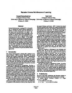
Environment
observation, reward
– Agent + Environment
action
– Agent selects actions to maximize utility function. Agent
3
RL system circa 1990’s: TD-Gammon Reward function: +100 if win - 100 if lose 0 for all other states
Trained by playing 1.5x10⁶ million games against itself. Enough to beat the best human player.
4
2016: World Go Champion Beaten by Deep Learning
5
RL applications at RLDM 2017 • • • • • • • • • •
Robotics Video games Conversational systems Medical intervention Algorithm improvement Improvisational theatre Autonomous driving Prosthetic arm control Financial trading Query completion
6
When to use RL? •
Data in the form of trajectories.
•
Need to make a sequence of (related) decisions.
•
Observe (partial, noisy) feedback to choice of actions.
•
Tasks that require both learning and planning.
7
RL vs supervised learning Training signal = desired (target outputs), e.g. class
Inputs
Supervised Learning
Outputs
Training signal = “rewards”
Inputs (“states”)
Reinforcement Learning
Outputs (“actions”)
8
RL vs supervised learning Training signal = desired (target outputs), e.g. class
Inputs
Supervised Learning
Training signal = “rewards”
Inputs (“states”)
Reinforcement Learning
Outputs
Environment
Outputs (“actions”)
9
RL vs supervised learning Training signal = desired (target outputs), e.g. class
Inputs
Supervised Learning
Training signal = “rewards”
Inputs (“states”)
Reinforcement Learning
Outputs
Environment
Outputs (“actions”)
10
Practical & technical challenges: 1. Need access to the environment. 2. Jointly learning AND planning from correlated samples. 3. Data distribution changes with action choice.
Markov Decision Process (MDP) Defined by: S: = {s1, s2, …, sn }, the set of states (can be infinite/continuous) A: = {a1, a2, …, am }, the set of actions (can be infinite/continuous) T(s,a,s’) := Pr(s’|s,a), the dynamics of the environment
MDPs as Decision Graphs
R(s,a): Reward function μ(s) : Initial state distribution
&"
&#
T
!"
!#
%#
11
T
!$
%$
'''
The Markov property The distribution over future states depends only on the present state and action, not on any other previous event. Pr(st+1 | s0, …, st, a0, … MDPs at) = Pr(st+1 t , at ) as| sDecision &"
Graphs
&#
!"
12
!#
!$
%#
%$
'''
The Markov property •
Traffic lights?
•
Chess?
13
The Markov property •
Traffic lights?
•
Chess?
•
Poker?
Tip: Incorporate past observations in the state to have sufficient information to predict next state. 14
The goal of RL? Maximize return! •
Return, Ut of a trajectory, is the sum of rewards starting from step t.
15
The goal of RL? Maximize return! •
Return, Ut of a trajectory, is the sum of rewards starting from step t.
•
Episodic task: consider return over finite horizon (e.g. games, maze).
Ut = rt + rt+1 + rt+2 + … + rT
•
Continuing task: consider return over infinite horizon (e.g. juggling, balancing).
Ut = rt + grt+1 + g2rt+2 + g3rt+3 … = ∑k=0: ∞ gkrt+k 16
The discount factor, g •
Discount factor, g ∊ [0, 1) (usually close to 1).
•
Intuition: – Receiving $80 today is worth the same as $100 tomorrow (assuming a discount factor of factor of g = 0.8). – At each time step, there is a 1- g chance that the agent dies, and does not receive rewards afterwards.
17
Defining behavior: The policy •
Policy, p defines the action-selection strategy at every state:
p(s,a) = P(at=a | st=s) p : S→A
Goal: Find the policy that maximizes expected total reward. (But there are many policies!) argmaxp Ep [ r0 + r1 + … + rT | s0 ]
18
Example: Career Options
n,a Unemployed
n,i
i
Example: Career Options Industry
0.8
0.2
gUnemployed i 0.6 g a Industry r=!0.1 r=+10 i (I) (U)i Grad 0.4 Academia n School r=!1 a0.5 g,n
0.9
i
g
0.5
Grad School (G)
n=Do Nothing i = Apply to industry g = Apply to grad school a = Apply to academia
n,g,a
0.1 0.9 a
What is the best policy? 0.1
Academia (A)
19
r=+1
Example: Career Options 0.2
n,a Unemployed R(s) = -1
0.5
i
g
g,n
Industry R(s) = +10 0.2
0.5
0.8
g 0.6 0.4 Unemployed
(U)i Grad n School r=!1 R(s) = 0
n,i
Example: Career Options 0.9
r=!0.1
0.8
i
0.7
g 0.6
0.6 0.4 a0.5 0.4
i
0.5
Grad School (G)
a Industry 0.9 i 0.1 r=+10 (I) Academia R(s) 0.9 = +5 n,g,a
0.1 0.9 a
What is the best policy? 0.1
n=Do Nothing i = Apply to industry g = Apply to grad school a = Apply to academia
Academia (A)
20
r=+1
Value functions
The expected return of a policy (for every state) is called the value function: Vp(s) = Ep [rt + rt+t + … + rT | st = s ]
Simple strategy to find the best policy: 1. Enumerate the space of all possible policies. 2. Estimate the expected return of each one. 3. Keep the policy that has maximum expected return.
21
Getting confused with terminology? •
Reward?
•
Return?
•
Value?
•
Utility?
22
Getting confused with terminology? •
Reward: 1 step numerical feedback
•
Return: Sum of rewards over the agent’s trajectory.
•
Value: Expected sum of rewards over the agent’s trajector.
•
Utility: Numerical function representing preferences.
•
In RL, we assume Utility = Return.
23
The value of a policy Vp(s) = Ep [rt + rt+1 + … + rT | st = s ] Vp(s) = Ep [rt ] + Ep [ rt+1 + … + rT | st = s ] Vp(s) = ∑aÎA p(s,a)R(s,a) + Ep [ rt+1 + … + rT | st = s ] Immediate reward
Future expected sum of rewards
24
The value of a policy Vp(s) = Ep [rt + rt+1 + … + rT | st = s ] Vp(s) = Ep [rt ] + Ep [ rt+1 + … + rT | st = s ] Vp(s) = ∑aÎA p(s,a)R(s,a) + Ep [ rt+1 + … + rT | st = s ] Vp(s) = ∑aÎA p(s,a)R(s,a) + ∑aÎA p(s,a)∑s’ÎST(s,a,s’)Ep [rt+1+…+ rT | st+1=s’ ] Expectation over 1-step transition
25
The value of a policy Vp(s) = Ep [rt + rt+1 + … + rT | st = s ] Vp(s) = Ep [rt ] + Ep [ rt+1 + … + rT | st = s ] Vp(s) = ∑aÎA p(s,a)R(s,a) + Ep [ rt+1 + … + rT | st = s ] Vp(s) = ∑aÎA p(s,a)R(s,a) + ∑aÎA p(s,a)∑s’ÎST(s,a,s’)Ep [rt+1+…+ rT | st+1=s’ ] Vp(s) = ∑aÎA p(s,a)R(s,a) + ∑aÎA p(s,a)∑s’ÎST(s,a,s’) Vp(s’) By definition
This is a dynamic programming algorithm. 26
The value of a policy State value function (for a fixed policy): Vp(s) = ∑aÎA p(s,a) [ R(s,a) + g ∑s’ÎS T(s,a,s’)Vp(s’) ] Immediate
Future expected sum of rewards
State-action value function: Qp(s,a) = R(s,a) + γ ∑s’T(s,a,s’)[∑a’ÎA p(s’,a’)Qp(s’,a’)] These are two forms of Bellman’s equation. 27
The value of a policy State value function: Vp(s) = ∑aÎA p(s,a) ( R(s,a) + g ∑s’ÎS T(s,a,s’)Vp(s’) ) When S is a finite set of states, this is a system of linear equations (one per state) with a unique solution Vp. Bellman’s equation in matrix form:
Vp = R p + g Tp Vp
Which can solved exactly:
Vp = ( I - g Tp )-1 Rp
28
Iterative Policy Evaluation: Fixed policy Main idea: turn Bellman equations into update rules.
1. Start with some initial guess V0(s),∀s. (Can be 0, or r(s,·).)
29
Iterative Policy Evaluation: Fixed policy Main idea: turn Bellman equations into update rules.
1. Start with some initial guess V0(s),∀s. (Can be 0, or r(s,·).)
2. During every iteration k, update the value function for all states: Vk+1(s) ¬ ( R(s, p(s)) + g ∑s’ÎS T(s, p(s), s’)Vk(s’) )
30
Iterative Policy Evaluation: Fixed policy Main idea: turn Bellman equations into update rules.
1. Start with some initial guess V0(s),∀s. (Can be 0, or r(s,·).)
2. During every iteration k, update the value function for all states: Vk+1(s) ¬ ( R(s, p(s)) + g ∑s’ÎS T(s, p(s), s’)Vk(s’) )
3. Stop when the maximum changes between two iterations is smaller than a desired threshold (the values stop changing.) This is a dynamic programming algorithm. Guaranteed to converge! 31
Convergence of Iterative Policy Evaluation •
Consider the absolute error in our estimate Vk+1(s):
•
As long as ga rt, st+1
49
Online reinforcement learning •
Monte-Carlo value estimate: Use the empirical return, U(st) as a target estimate for the actual value function:
V (st ) ← V (st ) + α (U(st ) −V (st ))
* Not a Bellman equation. More like a gradient equation.
– Here 𝛼 is the learning rate (a parameter). – Need to wait until the end of the trajectory to compute U(st).
50
Temporal-Difference (TD) learning •
Temporal-Di↵erence (Sutton, Monte-Carlo learning: V (st )(TD) ← V (stLearning ) + α (U(st ) −V (st ))
1988)
We want to update the prediction for the value function based on its change, i.e. temporal di↵erence from one moment to the next Tabular TD(0): • • TD-learning: V (st)
V (st) + ↵ (rt+1 + V (st+1)
V (st)) 8t = 0, 1, 2, . . .
TD-error
• Gradient-descent TD(0): If V is represented using a parametric function approximator, e..g a learning neural network, with parameter ✓: rate ✓
✓ + ↵ (rt+1 + V (st+1) 51
V (st)) r✓ V (st), 8t = 0, 1, 2, . . .
TD-Gammon (Tesauro, 1992) Reward function: +100 if win - 100 if lose 0 for all other states
Trained by playing 1.5x10⁶ million games against itself. Enough to beat the best human player.
52
Several challenges in RL •
Designing the problem domain – State representation – Action choice – Cost/reward signal
•
Acquiring data for training – Exploration / exploitation – High cost actions
•
Time-delayed cost/reward signal
•
Function approximation
•
Validation / confidence measures 53
Tabular / Function approximation •
Tabular: Can store in memory a list of the states and their value. * Can prove many more theoretical properties in this case, about convergence, sample complexity.
0.1 0.7 Intended direction
0.1 0.1
•
Function approximation: Too many states, continuous state spaces.
54
In large state spaces: Need approximation
55
Learning representations for RL
s
Q𝛳(s,a)
Original state
Linear function
56
Deep Reinforcement Learning s
Q𝛳(s,a)
Original state
Convolutional Neural Net
Deep Q-Network trained with stochastic gradient descent. [DeepMind: Mnih et al., 2015]. 57
Deep RL in Minecraft
Many possible architectures, incl. memory and context Online videos: https://sites.google.com/a/umich.edu/junhyuk-oh/icml2016-minecraft [U.Michigan: Oh et al., 2016]. 58
The RL lingo •
Episodic / Continuing task
•
Batch / Online
•
On-policy / Off-policy
•
Exploration / Exploitation
•
Model-based / Model-free
•
Policy optimization / Value function methods
59
On-policy / Off-policy •
Policy induces a distribution over the states (data). – Data distribution changes every time you change the policy!
60
On-policy / Off-policy •
Policy induces a distribution over the states (data). – Data distribution changes every time you change the policy!
•
Evaluating several policies with the same batch: – Need very big batch! – Need policy to adequately cover all (s,a) pairs.
61
On-policy / Off-policy •
Policy induces a distribution over the states (data). – Data distribution changes every time you change the policy!
•
Evaluating several policies with the same batch: – Need very big batch! – Need policy to adequately cover all (s,a) pairs.
•
Use importance sampling to reweigh data samples to compute unbiased estimates of a new policy.
62
Exploration / Exploitation
63
Exploration / Exploitation Exploration: Increase knowledge for long-term gain, possibly at the expense of short-term gain
Exploitation: Leverage current knowledge to maximize short-term gain
64
Model-based vs Model-free RL
•
Option #1: Collect large amounts of observed trajectories. Learn an approximate model of the dynamics (e.g. with supervised learning). Pretend the model is correct and apply value iteration.
•
Option #2: Use data to directly learn the value function or optimal policy.
65
Approaches to RL Policy Optimization / Value Function
Policy Optimization
Dynamic Programming modified policy iteration
DFO / Evolution
Policy Gradients
Policy Iteration
Value Iteration
Q-Learning Actor-Critic Methods
66
TD-Learning
Quick summary •
RL problems are everywhere! – Games, text, robotics, medicine, …
•
Need access to the “environment” to generate samples. – Most recent results make extensive use of a simulator.
•
Feasible methods for large, complex tasks.
•
Intuition about what is “easy”, “hard” is different than supervised learning.
Learning RL 67
Planning
RL resources Comprehensive list of resources: • https://github.com/aikorea/awesome-rl
Environments & algorithms: • http://glue.rl-community.org/wiki/Main_Page • https://gym.openai.com • https://github.com/deepmind/lab
68