Reinforcement Learning Real Experiments for Opportunistic ... - Supelec

Reinforcement Learning Real Experiments for Opportunistic Spectrum Access Christophe MOY SUPELEC/IETR Avenue de la Boulaie, 35576 Cesson-Sévigné, France [email protected] Abstract-- This paper proposes the analysis of experimental results obtained on the first worldwide implementation on real signals of reinforcement learning algorithms used for cognitive radio decision making in an opportunistic spectrum access (OSA) context. Two algorithms, able to act in highly unpredictable conditions, are compared: UCB (Upper Confidence Bound) and WD (Weight Driven). The OSA scenario is played in lab conditions around a couple of USRP N210 platforms. One platform is playing the role of the primary network and generates signals in a set of frequency bands with a pre-defined mean vacancy probability for each. An OFDM modulation scheme is used here, generated with GRC environment (GNU Radio Companion). Another platform runs Simulink in order to play the role of the secondary user (SU) cognitive engine that learns. The experimental results shown in this paper illustrate how the SU learns and predicts the channels’ vacancy thanks to UCB and WD algorithms. They validate in real conditions machine learning algorithms capabilities for opportunistic spectrum access context, in terms of learning speed and convergence accuracy. They enable also to compare UCB and WD performance. Index terms-- cognitive radio, OSA, reinforcement learning, UCB, weight-driven, decision making, convergence

I.

INTRODUCTION

Learning is one of the main features a radio equipment should have in order to turn it towards cognitive radio. This sentence can be applied at network level as well, and then we speak about cognitive networks. Cognitive radio paradigm is all about providing self-adaptation capabilities to the radio equipments and networks so that they can adapt dynamically to real-time conditions. Current usual radio systems however are designed to support the worst case situation they are supposed to face rarely, which results at almost all instants in a loss in terms of power consumption, autonomy, spectrum efficiency and consequently capacity of the global system, etc. In other words, current radio systems are far from optimality, whatever the goal criteria, and cognitive radio is a way to make a further step towards

optimality. The facilities a cognitive radio equipment (or a cognitive network) should include in addition to usual radio processing any radio equipment should have [1], can be summarized as [2]: - sensing means, - learning and decision making means, - adapting means. Many studies have been done and many papers have been published for the past twenty years on the third part, in other words software radio. Sensing has been also a major focus in the community for the last ten years. Decision has often been considered as an optimization issue in an expert system perspective [3]. But not so many papers have been done on learning for cognitive radio, and none on implementing learning in real wireless conditions. This paper aims at deeply analyzing results of the first worldwide implementation of reinforcement learning (RL) algorithms for OSA (opportunistic spectrum access) on real radio signals. Two reinforcement learning algorithms, UCB (Upper Confidence Bound) and WD (Weight Driven), are used by a secondary user (SU) to learn about channels occupancy in order to derive the best channel to select in an OSA scenario. The considered learning algorithms are able to act in highly unpredictable conditions, e.g. learn from scratch about the spectrum occupancy by primary users (PU). This paper is organised as follows. Secion II deals with spectrum learning and section III makes a focus on reinforcement learning for OSA. Then the experimental context is presented in section IV. Sections V and VI propose an analysis of experimental results obtained so far. Learning speed, convergence properties, as well as a comparison between UCB and WD are discussed before drawing some conclusion.

II. LEARNING SPECTRUM FOR COGNITIVE RADIO A. Decision Making vs Learning We focus in this paper on the decision making and learning attributes. They hardly can be divided as they are intimately inter-related. Paper [3] makes an overview of decision making strategies that have been studied during the first ten years of CR. To sum-up, in order to select which decision strategy is appropriate for a given CR context, it is necessary to analyze the degree of a priori knowledge the system has on its environment (in the widest sense of [1] and [2]). If the system perfectly knows the environment state (which can be derived from many parameters), expert schemes can be used. In this context indeed, the system configuration corresponding to each environment state can be pre-defined a priori. At the opposite, when the environment state is unpredictable instantaneously, or at least when it is statistically predictable, learning is helpful. This paper deals with this case, which is the hardest met in CR scenarios. B. Opportunistic spectrum access Radiofrequency spectrum is a rare, then expensive resource. During the 20th century, spectrum scarcity issue has been solved by exploiting always new higher frequency bands thanks to electronics progresses. Improvements have been also made by the signal processing research community during this period: more information could be sent in the same bandwidth, or bandwidth could be reduced for the same amount of data to be sent in a second. Despite all these progresses however, wireless applications’ demand is growing faster than the new spectrum opportunities. Consequently spectrum scarcity is even worse every year. We are facing such a limit today that spectrum access paradigm needs to be changed. We should now move indeed from improvement to a real breakdown of spectrum related issue. Many measurements indeed have shown recently that if all spectrum bands are reserved for a specific service or application, many of them are underused in time [4][5], depending on each location. Then an opportunity exists for new spectrum if spectrum sharing is done differently [6]. OSA is one of them. It consists in enabling Secondary Users (SUs) to use the spectrum let vacant by licensed Primary Users (PUs).

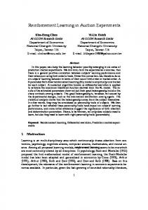
Cognitive radio [1], through its features in terms of permanent adaptability to varying conditions, is foreseen as key technology in order to implement such new schemes in commercial and military spectrum. In an OSA commercial context, this is derived as follows: time is slotted in iterations. At each iteration, the SU radio system senses a channel. Either the channel is detected vacant and then transmission is done by the SU system on this channel. Or the channel is detected occupied and no transmission is done at that iteration. The SU system must wait for next iteration to sense another channel. Learning consists in taking into account the past trials’ results in order to decide which channel to target at next iteration. The goal is to maximize the probability of success (e.g. channel is vacant) in order to maximize transmission opportunities for SU. C. Reinforcement Learning for OSA RL is based on the “try and evaluate” principle which consists in iteratively trying a set of solutions, evaluating their result and then deriving some quality factor of each trial. The goal is to order solutions, given a quality objective, so that the best one is used at next iteration. In other words, this aims at predicting which solution is giving the best opportunity at next trial. Figure 1 shows how this can be derived in the OSA context, at the output of a sensing algorithm detecting the presence of a PU signal (energy detector, cyclostationnarity detector, etc.). The learning and decision process aims at: 1. deciding to transmit or not at current iteration, 2. updating learning information, 3. deciding which channel to sense and to choose for transmission at next iteration. The decision to transmit is done only if the detection finds the channel vacant at the current iteration. Learning, as well as the decision on which channel to try to transmit at next iteration, are done whatever the detection result. The OSA context can be modeled as a MAB issue (Multi-Armed Bandit) [7]. In the OSA context, the MAB model is the following: each frequency channel is equivalent to a gambling machine or a bandit arm. If we consider a wide sense stationnary context, the figure of merit of a channel is its probability of vacancy, e.g. not used by a PU, which is equivalent to the probability for a gambling machine or arm to win.

update knowledge

DECISION

LEARNING next iteration channel choice

PU yes do not transmit detected? no

transmit in sensed channel

Figure 1 - Learning and decision making processes based on a reinforcement learning approach in OSA context.

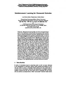
D. Implementation perspectives for OSA The advantage of the proposed RL algorithm for OSA is that in such an approach only one channel is sensed at a time. It is indeed a MAB context as you only play one gambling machine at a time in casino. Then Radio Frequency (RF) front-end and digital processing front-end of the radio do not have to support a larger bandwidth than the bandwidth of one channel which is required for the transmission itself. In other words, there is no need for a wideband RF (and the associated digital processing power) to sense all channels of interest in parallel, which represents great savings both at design and operation times. As shown in Figure 2, the proposed OSA radio equipment can be based on a conventional radio with the only addition of sensing, decision making and learning components. RX RF processing

sensing

TX RF processing

paper. Here, we assume that the conventional radio system is able to change of channel, e.g. its carrier frequency statically. In other words, it selects a frequency at the beginning of each communication, but does not change during communications. Therefore, ‘adapt’ block here just uses differently a feature that is present in the conventional radio. It is not a new feature to be added for OSA purposes only.

RX baseband processing

learning decision

adapt

TX baseband processing

Figure 2 - Cognitive cycle elements to be added to a conventional radio to support the proposed OSA features are highlighted in dark grey.

As a consequence, OSA introduction does not require changing the global design of the equipments, but just add some light digital signal processing as it will be shown in the experiments at the end of the

III. REINFORCEMENT LEARNING ALGORITHMS FOR OSA We also aim in this study at comparing on real radio signals two RL algorithms which have been proposed for OSA. UCB algorithm we have been studying theoretically in [8] is the first one. The second is the Weight Driven algorithm proposed in [9]. A. RL model for OSA The spectrum is divided in K channels denominated by k Є {1, 2, …, K}, each having the same bandwidth and representing one arm for the MAB algorithm. We suppose that time is discrete, slotted in iterations, and that only one channel is sensed at each iteration. The temporal occupancy of every channels follows a Bernoulli distribution θk for which the mean expected value, µ k = E[θk], can be set independently in simulations and in the experiments. The SUs are supposed to be synchronous with PUs. We define t as the discrete time index representing the total number of times (or iterations) that the algorithm has been played. The cumulative number of times that channel k has been chosen in the previous steps is Tk. B. Upper Confidence Bound Algorithm for OSA We have been studying for several years at theoretical level the potential capabilities of UCB algorithms as a means for a CR equipment to learn about spectrum opportunities. UCB is a RL algorithm that can solve problems modeled as MAB. It has been explained in [3] that this kind of approach is efficient in a context of high uncertainty, e.g. where the cognitive system has no a priori knowledge about the channel occupancy statistics. UCB has been identified indeed at the beginning as a solution for decentralized learning for cognitive radio [8]. Then, UCB has been confronted to sensing

errors and cooperative mechanisms, which has confirmed their validity in the cognitive radio context. It has been proven theoretically in [10] that UCB still converges to the best solution(s) if sensing errors are committed. Then simulations on a radio chain have been derived to confirm the validity of the theoretical results, taking into account sensing errors of energy detector for instance. There exists several UCB [11] algorithms but that does not change the generality of the proposed approach. Let’s state that an independent realization ,

( )

of the statistical distribution θk described ,

previously has an empirical sample mean

( )

. If

we define , , ( ) as a bias added to the empirical sample mean, we can compute UCB coefficients , ,

( )

as in [12] for UCB1 with: , ,

and

, ,

( ) ( )

← ←

α ln ( ) ,∀ ( )

,

( )

+

, ,

( )

Wt+1,k = Wt,k + f

,∀

returns the index of the maximum value of , ,

( )

The WD algorithm is structured the same way as UCB except for three aspects: - Bk index of each channel is replaced here by a weight Wk which is not based on the empirical mean, but only a function of the number of times this channel has been sensed vacant and occupied, - the introduction of a preferred set of channels reduces the set of possibly selected channels to a subset of the total number of channels, this subset selecting the best channels obtained after a given initialization step [9], - the decision to transmit is not only based on the presence or not of the primary user in [9]. It is also a function of the quality of the considered channel, but this will not be considered in this paper. After each trial, the weight of the channel k that has been chosen for transmission is updated as follows:

At each iteration, decision based on UCB algorithm Indeed

C. Weight Driven Algorithm for OSA

, ,

( ).

indexes are constituted for each

, ( ) (obtained on channel of the empirical mean the trials made on each channel) upper bounded by a

, , ( ) bias (specific to each channel also). The higher the Bk index of a channel, the higher probability this channel is to be vacant. So the SU will choose to transmit at next iteration on the channel having the highest Bk index. A consequence is that the best channels are also more sensed than others and the knowledge on their availability is closer to reality. Note also that coefficient α is relative to the speed of convergence of the algorithm. In other words, α sets the relative ratio between exploration and exploitation. A lower α decreases the influence of the bias

compared to the vacancy empirical mean . Then a lower α makes UCB give more confidence on its paste experience and favor exploration. At the opposite, a higher α favors exploration by increasing impact.

where f = +1 if the channel is rewarded, e.g. detected vacant, and f = -1 if it is punished, e.g. detected occupied. Note that if Wk is null and channel k is detected occupied, Wk stays null (Wk ≥ 0). Each channel is ranked thanks to its weight which reflects the quality of the resource. The WD algorithm is directly derived from the two stages RL algorithms proposed in [13]. The decision process is based on a statistical distribution constructed from the weights:

( )=

∑

1,…,

,

,

where Pt(k) is the probability that the channel k is chosen. Moreover WD’s choice does not directly consist in selecting the channel with the highest weight. If the weight of a channel is above a given threshold Vt, then the channel is selected to enter the preferred set. When the preferred set is full, the choice is restricted to the channels in the set. A new channel may be included in the preferred set only if another is leaving it while its Wk is decreasing under the threshold value. The threshold value and the size of the preferred set are the parameters which dimension the WD algorithm in terms of exploration and exploitation.

IV. EXPERIMENTAL CONTEXT A. Primary user network platform In our experiments, the primary network is made of 8 channels, e.g. K = 8. The probability of vacancy of each channel by the primary users can be set as wanted and has been chosen as follows in the following experimental results of this paper: {0.5;0.3;0.4;0.5;0.6;0.7;0.8;0.9}. This means that the probability of occupancy of channel 1 by PUs is 0.5, the probability of occupancy of channel 2 by PUs is 0.7, the probability of occupancy of channel 3 by PUs is 0.6, and so on until the probability of occupancy of channel 8 which is 0.1 only. So channel 8 has a probability of vacancy of 90% and then is the best channel to offer secondary transmissions opportunities. Instead of using 8 platforms that should be synchronized to coordinate primary users frequency jumps, an OFDM signal generation with 8 carriers has been chosen [14]. Only one platform is necessary and the synchronization between users is straightforward as all channels traffic is generated through OFDM symbols. Switching-on and off channels only consists in filling the 8 elements vector before the IFFT by a “1” when a channel should be occupied and “0” when it should be vacant. Hence channels 1, 5, 7 and 8 are vacant in the vector [0 ; 1 ; 1 ; 1 ; 0 ; 1 ; 0 ; 0].

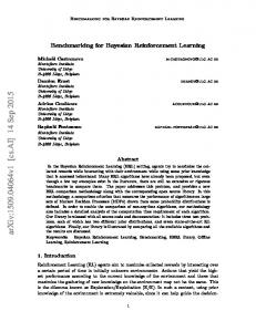
The chosen design environment for the primary network radio signal generation is GNU Radio Companion (GRC) and the hardware platform is made of a USRP platform from Ettus Research [15] connected to a laptop running Linux as shown left hand side of Figure 3. For simplicity purposes, OFDM symbols rate is set to one symbol per second. This means that the channel occupancy of PUs varies once a second and can be followed by human eye. Nothing technically prevents form accelerating this rate. Algorithms converge in function of the number of trials, so learning algorithms convergence speed is directly a function of this rate. If frames would be 1 ms long, we could directly conclude on a learning speed 1000 times faster than the current experiment. B. Secondary user platform The right hand side platform of Figure 3, made of a computer and a USRP platform, represents a secondary user. Only sensing and learning are implemented here, e.g. this platform is only a receiver (RX). In other words, the decision to transmit, after detecting the channel is empty, is not implemented here and no SU transmission occurs. This is out of the scope of our experiment which focuses in learning validation.

Figure 3 – Experimental testbed for learning in an OSA context. Left hand side (laptop + USRP) is the playing the role of the primary network transmission (TX) with the visualization of the generated traffic on 8 channels. Right hand side (laptop + USRP) is the playing the role of the secondary user learning algorithm, implementing an energy detector as a sensor (RX).

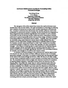
The detector for sensing is an energy detector, but any other detector could be used without any loss of generality on the learning results. Sensing quality may have an influence but what is important in the experiment is that there may be errors of detection, as it can be expected in the reality, e.g. SU decides a PU is present when it is not (false alarm), or SU decides a PU is not present when it is (misdetection). Channel number 1 is used as a synchronization means for the secondary user platform. The occupancy probability of channel 1 is 0.5 as it is switching from vacant to occupied and vice-versa at each OFDM symbol. This enables the secondary user to detect when the transition between OFDM symbols is done so that the SU synchronizes the energy detection phase on an entire OFDM symbol of the primary network. V. EXPERIMENTAL RESULTS ANALYSIS Figure 4 is snapshot of the secondary user host PC screen that shows the results for an experiment shot after 350 iterations. The left hand side curve displays , the empirical vacancy probability of channels derived from UCB during the first 350 iterations of a shot, whereas right hand side curve displays UCB indexes evolution during the same period of time. We discuss about these results after next section which describes the tables formats. A. Table results format Tables in the middle of Figure 4 show figures concerning WD algorithm at the top and UCB at the bottom.

For both algorithms, tables are ordered from channel 1 to 8 starting at the top. WD algorithm table is the top one with the following information: - central column is the number of times WD algorithm played each channel, - right column is the weight Wk of each channel, consequently a function of the difference between the number of times the channel was detected vacant with the number of times it was detected occupied, - left column is the empirical probability of vacancy of the channels. It is given for information purposes, in order to compare with the real probability given in section IV.A and the one obtained with UCB. It is not a parameter used by WD algorithm. Concerning UCB algorithm, just two columns are given in the bottom table: - right column is the number of times UCB algorithm played each channel, - left column is the empirical probability of vacancy of the channels , from which Bk index value is derived for each channel. Channels with a higher Bk and Wk index are more played compared to those with a low index. This means that the channels which are the most likely to be vacant are more sensed in order to obtain more transmission opportunities. Only one channel is sensed at each slot indeed and only this one can be used for transmission at the current iteration. Note that in this experiment, both algorithms are executed in parallel, on exactly the same experimental data in terms of carrier randomness and radio channel conditions. However, the choice of the channel selected at each iteration is different since these algorithm follow different strategies.

Figure 4 - Evolution during first 350 iterations of an experiment shot. Left hand side: empirical average vacancy rate of the 8 channels derived from UCB. Right hand side: UCB indexes evolution. Bottom middle table: UCB trials on the right column and derived channels average vacancy rate at iteration 350. Top middle table: WD weights in the right column, number of WD trials in the middle and derived channels average vacancy rate in the right column.

B. Learning Speed analysis One goal of this experiment is to evaluate the speed of the learning process in real radio conditions. Do reinforcement learning algorithms make sense for cognitive radio applications? Figure 5 is another example, equivalent to left Figure 4, that shows the very beginning of the learning process with UCB algorithm. Both experiments have been done with the same channel vacancy rates given in section IV.A, but different random samples. We can see that the beahvior is roughly the same, but with different results because of randomness effects. The main point to emphasize is that just after a few hundreds of iterations, we of real obtain a quite accurate approximation vacancy probability of channels, e.g. in Figure 5: - 0.91 for channel #8 in violet instead of 0,9; - 0.87 for channel #7 in yellow instead of 0,8; - 0.8 for channel #6 in dark blue instead of 0,7; - 0.74 for channel #5 in green instead of 0,6; - 0.58 for channel #4 in red instead of 0,5; - 0.68 for channel #3 in light blue instead of 0,4; - 0.14 for channel #2 in purple instead of 0,3; - 0.69 for channel #1 in yellow instead of 0,5; These are amazing results as this kind of reinforcement learning algorithm, which is based on a convergence at infinite time, are very rapidly accurate. We can see on Figure 5, that after just one third of these iterations, just a little bit more than 100 iterations, these results are almost obtained.

Figure 5 – Empirical probability of vacancy of the eight channels derived by UCB algorithm during 340 iterations: channel #8 is violet / #7 yellow / #6 blue / #5 green / #4 red / #3 light blue / #2 purple / #1 light yellow

If iterations occur at a rate of 1 ms (a typical frame size as in 4G LTE wireless standard), this means that these results can be obtained after 100 ms only. Of course, if a greater number of channels is considered, learning should be proportionnally longer to obtain the same results. A hundred channels would be “learnt” at the same level in a little bit more than 1 s. Moreover, most important is not to derive the exact probability of vacancy, but to derive the channel hierarchy in terms of transmissions opportunities. Bk indexes of UCB are not reflecting exactly the probability of vacancy, but a value relative to the empirical probability of vacancy k, biased with Ak factor. The Bk indexes evolution is harder to interpret intuitively, but can be seen on the right curve of Figure 4. Fast increment or decrement phases correspond to a period where the channel of interest is selected for sensing. If it is sensed vacant (respectively occupied), its Bk index increases (respectively decreases) fast, so that one after another, each Bk index is becoming the greatest and then is selected from time to time. However, more selection occurrences happen for those having a good empirical mean on past experiments, and less occurrence for those having a bad empirical mean on past experiments. C. Convergence issue Following figures detail on a few steps how learning progresses. We can see on Figure 6 the very beginning of the learning phase, e.g. after 80 trials (a mean of 10 trials per channel then). We just consider the best channel first, which is channel number 8 at the bottom of each table. On this example, whereas UCB algorithm is only theoretically guaranteed to converge at infinity, we can see that it has already chosen almost one third of the time the most available channel (channel 8). This maximizes the transmission opportunities, as channel 8 has a 90% probability of being vacant, compared to a uniform rule which would have selected this channel only 1/8 of the times. WD algorithm on its side is still filling its preferred set, which is set at 3 in these experiments. During this time WD operates as UCB and can exploit the channel when it is vacant, but it seems that WD has not selected the best channel in its preferred set. We can see that WD tried two times the best channel but it was occupied once, so it has been overpassed by other channels which were vacant in the early trials, so that it is not favored.

Figure 6 - Learning results on the eight bands after 80 iterations – top table for WD algorithm and bottom table for UCB algorithm

Figure 7 is extracted from the same shot as Figure 6 after 1500 trials. Figure 7, and later Figure 8, confirm that WD has not selected the best channel in its preferred set. It is then very hard to change the preferred set as it means that one of the selectd channels should be detected occupied as many times as it has been detected vacant before. Then its weight value decreases under the threshold value and consequently WD can explore again other channels and see which one to integrate in the preferred set. D. Impact of sensing errors Sensing errors are committed, but the current experimental protocol can not allow to derive the exact probability of false alarm and misdetection. This is a future work we are working on currently. However, as the left column of the two tables of Figure 6 to Figure 8 are displaying the empirical probability derived from past experiments, we can see that they are not exactly equal to those defined arbitrarily for the primary network channels’ vacancy. Results obtained after 7000 iterations are given in Table 1 (derived from Figure 8). Note that for WD, we only filled channels that have been deeply explored, e.g. those of the preferred set.

Figure 7 - Learning results after 1500 iterations

We can see that experimental results are a little bit too much optimistic in general, which could emphasize a certain probability of misdetection. However, we can not definitely state on the real causes in this experimental context. Future work will do. Table 1 - Empirical probability of vacancy (EPV) derived by UCB and WD after 7000 iterations, compared to the probability of vacancy set in the experiments (PVSE) channel #8 #7 #6 #5 #4 #3 #2 #1

EPV UCB 0.87 0.84 0.80 0.79 0.57 0.53 0.27 0.70

EPV WD 0.82 0.77 0.72

PVSE 0.90 0.80 0.70 0.60 0.50 0.40 0.30 0.50

E. Extra-computational power for supporting CR Sensing and learning signal processing is so simple that it can be done in real time using Simulink on a conventional laptop. We have usually experienced a factor 60 between Simulink and GRC execution speed in favor of GRC. Most of the processing is used for sensing and displaying

purposes. Learning only consists in updating a set of 8 figures requiring a square root operator for UCB and a few multiplications and additions for both. So both UCB and WD learning algorithms could be implemented in parallel with Simulink and without specific computing accelaration methods.

Figure 8 - Learning results after 7000 iterations

VI. UCB AND WD COMPARISON A. Comparison context Comparing two RL algorithms is expected to give information on their relative convergence speed and divergence characteristics. Moreover, it demonstrates reinforcement learning’s pertinence for cognitive radio. UCB and WD are only compared in these experiments in terms of learning based on the presence or not of a primary user. Other parameters concerning the quality of the channel (SINR) used by [13] associated with WD cannot be considered here as transmission is not implemented. So we just compare with UCB here the pure learning sub-part of WD, not the global WD approach of [13]. B. Convergence comparison We see on the experiments that WD may diverge, e.g. it may never converge on the best channel. This is the divergence criteria in terms of reinforcement

learning. This is what happens during our experiments when the best channel is not selected in the preferred set. This may be caused by the presence sensing errors. However, we have also experienced contexts without errors by simulation where WD diverges, just due to bad luck in randomness during initialization phase consisting in filling the preferred set. WD algorithm has indeed no mathematical proof of convergence, whereas UCB has been proven to be convergent for a perfect estimation (here detection of PU) by the machine learning community [12]. We have derived in our theoretical studies the proof of convergence of the UCB in presence of sensing errors on the PU presence [10]. This means that UCB algorithm guarantees to find the most available channel for an infinite time. The only concern is that for a given number of trials, the more sensing errors the longer it takes to converge. This has been verified on all the experimental shots we have done, even if only a few of them have provided data in this paper. These selected shots were typical shots, not special cases obtained rarely. C. Results Interpretation in terms of transmission opportunities Figure 6 to Figure 8 show how the SU learns in real-time and real radio signals the statistical mean of vacancy of primary channels thanks to RL. RL helps SU privileging at next transmission the use of the channels which have the best probability of being vacant. Hence after 7000 iterations, as shown in Figure 8, UCB has selected the best channel more than half of iterations. As this channel has a 90% probability of vacancy, this means that, in the worst case where all the other channels would be always occupied, SU has found transmission opportunities around 50% of the time. If the two best channels are considered, this increases up to ¾ of the attempts. Concerning WD algorithm, whereas it has diverged, results are even better than UCB if we consider the 4 best channels as they have been selected 100% of time. Indeed, number 2, 3 and 4 have been selected with a vacancy probability of respectively 0.8, 0.7 and 0.6, which offers also great transmission opportunities. This means that the convergence criteria, in the sense of machine learning, is not a criteria which is so valuable for cognitive radio real context. Machine learning

evaluation criteria versus cognitive radio’s ones is the topic of [16] if you want to read more about it. VII. CONCLUSION This paper presents the experimental results of the first implementation of reinforcement learning algorithms for CR on real radio signals. They demonstrate both accuracy and feasibility of RL for spectrum-oriented cognitive radio scenarios such as OSA. This experimental platform is a source for many further studies that could also help evaluating aspects of the cognitive radio chain complementary to learning. We are currently extending this demonstrator while integrating secondary transmission and feedback channel between secondary user and primary network platform so that probabilities of false alarm and misdetection can be measured. This will provide a very interesting experimental tooling for the evaluation of sensing algorithms in real radio conditions. VIII. ACKNOWLEDGMENT Author would like to thank Paul Sutton for advising the papers of the Trinity College of Dublin dealing with holes generation in OFDM spectrum. IX. REFERENCES [1] [2] [3]

[4] [5]

[6]

[7] [8]

J. Mitola, “Cognitive Radio” ” Licentiate proposal, KTH, Stockholm, Sweden, Dec. 1998. J. Palicot, "Radio Enineering: From Software radio to Cognitive Radio", Wiley 2011; ISBN: 978-1-84821-296-1 W. Jouini, C. Moy, J. Palicot, "Decision making for cognitive radio equipment: analysis of the first 10 years of exploration", EURASIP Journal on Wireless Communications and Networking 2012, 2012:26. "FCC Spectrum Policy Task Force: Report of the spectrum efficiency working group," 15 November 2002. M. López-Benítez, F. Casadevall, A. Umbert, J. PérezRomero, J. Palicot, C. Moy, R. Hachemani, “Spectral occupation measurements and blind standard recognition sensor for cognitive radio networks,” CrownCom, June 2009 Q. Zhao, A. Swami, "A Survey of Dynamic Spectrum Access: Signal Processing and Networking Perspectives", in IEEE ICASSP: special session on Signal Processing and Networking for Dynamic Spectrum Access, April, 2007 R. Agrawal, “Sample mean based index policies with o(log(n)) regret for the multi-armed bandit problem,” Advances in Applied Probability, 27:1054–1078, 1995 W. Jouini, D. Ernst, C. Moy, J. Palicot, "Upper confidence bound based decision making strategies and

dynamic spectrum access", ICC, Cape Town, South Africa, May 2010 [9] T. Jiang, D. Grace, P.D. Mitchell, “Efficient exploration in reinforcement learning-based cognitive radio spectrum sharing”, IET Communications, Aug. 2011. [10] W. Jouini, C. Moy, J. Palicot, "Upper Confidence Bound Algorithm for Opportunistic Spectrum Access with Sensing Errors", CrownCom'11, 1-3 June 2011, Osaka, Japan [11] J.-Y. Audibert, R. Munos, and C. Szepesvari. "Tuning bandit algorithms in stochastic en-vironments," International conference on Algorithmic Learning Theory, 2007. [12] P. Auer, N. Cesa-Bianchi, P. Fischer, “Finite time analysis of multi-armed bandit problems.”, Machine learning, 47(2/3):235-256, 2002. [13] T. Jiang, D. Grace, Y. Liu, “Two stage reinforcement learning based cognitive radio with exploration control”, IET Commun., 2011, 5, (5), pp. 644 – 651. [14] I. Macaluso, B. Özgül, K T. Forde, P. Sutton, L. Doyle, “Spectrum and Energy Efficient Block Edge MaskCompliant Waveforms for Dynamic Environments”. IEEE Journal on selected areas in communications, Vol. 32, No. 12, Dec. 2014 [15] Ettus Research “Products” - accessed 02/04/2012 http://www.ettus.com/products [16] C. Robert, C. Moy, C.X Wang, "Reinforcement Learning Approaches and Evaluation Criteria for Opportunistic Spectrum Access", IEEE ICC’14, International Conference on Communications, Sydney, Australia, 10-14 June 2014