Reject Options in Fuzzy Pattern Classification Rules - CiteSeerX

Reject Options in Fuzzy Pattern Classification Rules C. Fr´elicot(†)

M.H. Masson(‡)

B. Dubuisson(‡)

(†)

Laboratoire d’Informatique et d’Imagerie Industrielle, Universit´ e de La Rochelle, F-17042 La Rochelle Cedex 1, e-mail : [email protected]

(‡) U.R.A. C.N.R.S. Heuristique et Diagnostic des Syst` emes Complexes, Universit´ e de Technologie de Compi` egne, B.P. 649, F-60200 Compi` egne

Abstract The design of fuzzy pattern classification rules is presented. Since hard label transformation is not efficient for ill-defined and/or non-complete problems, we show how reject options can result in an attractive alternative. Different approaches are proposed and compared. Rules are derived and tested. Keywords : Classification rule design, Fuzzy classification, Reject options.

1

The Classification Problem

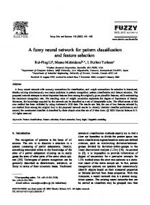
A pattern to be classified is an object described by d feature values, i.e. a d-dimensional vector x= (x1 x2 ... xd )t . Conventional pattern classification aims at associating each pattern to one of c predefined classes {ω1 , ω2 , ..., ωc } assumed to be representative of particular objects available from a learning set Ω = {x1 ,x1 , ...xn }. The classification is carried out on the base of class labels µi = µi (x) (i = 1, c). Hence, the classification problem consists, for each pattern x in : • computing a label vector µ(x)= (µ1 µ2 ... µc )t • designing a rule that assigns one label to x Each label value µi (i = 1, c) is in [0, 1]. It is called a fuzzy label when it can be interpreted as a membership hard labels corresponds to function value to the class ωi in the sense of the fuzzy sets theory. The case of P c the classical characteristic function value (µi ∈ {0, 1}). A normalization constraint i=1 µi is often set on the labels. We will discuss it later on. In case of fuzzy labelling, designing rules that transform fuzzy labels into hard ones can appear quite surprising. However, some authors claim that this is the only way to design a classifier. That is the reason why the so-called Maximum Membership Rule MMR is often used. It consists in defuzzyfying fuzzy labels as follows : ½ m = arg maxj=1,c µj (x) (1) µi ← δim where δim denotes the Kronecker symbol. It is worthy of note that ties must be arbitrarily broken. The rule results in partitioning the unit hypercube [0, 1]c where label vectors lie with bissecting hyperplanes. Figure 1 shows this classification boundary for the c = 2 classes problem. In our mind, classification based on fuzzy labels should not be an absolute quest for hard labels. The interest of a fuzzy approach in propagating uncertainties in decision processes has been widely proved. On the other hand, propagating information that is not ever relevant is not useful, particularly when one aims at automating the decision process. If so, hard classification is justified. A half-way approach can take place between both extreme trends. We will show it can be achieved by managing reject options in fuzzy classification rules. The goal of such an intermediate strategy is to transform fuzzy labels into hard ones but not at any cost.

µ 2 (x) 1

ω1 ω2

0 0

1

µ 1(x)

Figure 1: Classification areas (MMRule)

2

Reject options

Reject options have been introduced in pattern classification in order to decrease the misclassification risk. Two types of reject are under interest [DuM93] : • ambiguity reject • distance or membership reject The first one deals with the problem of ill-definition of the c classes issued from the learning set Ω. In this case, all the classes are not clearly separable and it is interesting to allow a pattern x to be classified into more than one class. Fuzzy labels clearly contain some ambiguity information. This kind of reject is not possible if hard labels are normalized. The second one deals with the problem of non-completeness of the learning set Ω. In that case, one or more classes are not known and it is interesting to allow a pattern x not to be classified into any of the c known classes. This kind of reject is not possible if the labels are normalized whatever they are fuzzy or hard.

3

Fuzzy Classification Rules with Reject Options

The straightforward way to introduce rejection in fuzzy classification rules is to threshold the fuzzy labels associated with the pattern x to be classified. What we will emphasize here is how membership and ambiguity rejects are introduced, .i.e. how the rule is designed. There are several ways to approach this design in fuzzy pattern classification : • sequential approach 1. membership reject : may x be assigned to one or several classes ? 2. ambiguity reject : if so, must x be assigned to one or more classes ? • parallel approach 1. reject : must x be assigned to one class ? 2. ambiguity/membership : if not, may x be assigned to more than one class or to none of them ? • implicit approach, introducing a membership reject class 1. may x be assigned to one class ? If not, it is implicitly ambiguity rejected. Depending of the chosen strategy, the classification rules differ even if it is always a matter of thresholding the fuzzy labels. The sequential approach is the most popular one because it is easy to formulate and implement.

3.1

A sequential approach

Such an approach deals with both kinds of reject at two sequential steps. The membership reject is first considered. If and only if the pattern x to be classified is not membership rejected from all the classes then the ambiguity reject is considered.

Assume one fixes, or computes from the learning set Ω, thresholds µ0,i (i = 1, c) such as the pattern x must be membership rejected from class ωi if its label is less than the corresponding threshold. Then, one can first transform the labels using : ½ 0 if µi (x) < µ0,i µi (x) ← (2) µi (x) otherwise Pc Membership reject happens if i=1 µi = 0. If not and only if not, one must distinguish the exclusive class assignment and the ambiguity rejection. For that purpose, it is possible to use a membership ratio as defined in [FrD93] by : µp (x) (3) R(x) = µm (x) where µm is defined as in eq. (1) and µp as µp (x) = maxj=1,c;j6=m µj (x). If R(x) → 0 then µm is far above all the others labels and x has not to be ambiguity rejected. Comparing R(x) to a fixed threshold Ra (0 ≤ Ra ≤ 1) allows a second transformation of the labels using : ½ δim if R(x) < Ra (4) µi (x) ← µi (x) otherwise Therefore, if x is not classified into class ωm , it is ambiguity rejected between all the classes it has not been membership rejected from. Note in that case initial labels remain. We call this rule the Membersip Ratio Rule (MRR). Figure 2 shows how the two sequential steps result in partitioning the unit hypercube [0, 1]c for the c = 2 classes problem ; ω0 and ωa stand for membership and ambiguity reject respectively. The less Ra , the more ambiguity. µ 2 (x) 1

ω0

Ra

1

ω1 ω2 ω0

Ra

µ 0,2

ωa

µ 0,2

0 0

µ 0,1

1

µ 1(x)

0 0

µ 0,1

1

µ 1(x )

Figure 2: Classification areas (MRRule)

3.2

A parallel approach

Such an approach deals with both kinds of reject at the same step. The exclusive classification or rejection is first considered. If and only if the pattern x to be classified is rejected then the distinction between ambiguity and membership reject is considered. Assume one fixes, or computes from the learning set Ω, thresholds µr,i (i = 1, c) and let us consider the following transformation :  ¾  µi (x) ← 1 if µi (x) > µr,i + maxj=1,c;j6=i µj (x) µj (x) ← 0 ∀j 6= i (5)  µi (x) ← µi (x) otherwise Thus, x is either rejected if no label changes or classified into a single class ωi . In case of rejection, one has to decide which kind it must be (ambiguity or membership). This can be achieved by introducing new thresholds µ0,i (i = 1, c). The labels of rejected patterns can be finally transformed using : ½ 0 if µi (x) ≤ µ0,i µi (x) ← (6) µi (x) otherwise

Pc x is membership rejected if i=1 µi = 0, else it is ambiguity rejected between all the classes it has non zero labels. Here again, initial labels remain in case of ambiguity rejection. Since thresholds µr,i are minima against rejection, we call this rule the minimum Maximum Rule (mMR). Figure 3 shows how the parallel approach for rejection results in partitioning the unit hypercube [0, 1]c for the c = 2 classes problem ; the less µ0,i , the more ambiguity. Obviously, if µ0,i = µr,i (∀i = 1, c), the rule could be described as a sequential one. A major difference with the previous rule is that ambiguity between learning classes and a fictive membership reject class is possible when µ0,i ≤ µr,i . It allows to manage simultaneously the ill-definition and the non-completeness of the learning classes. µ 2 (x)

µ 2 (x)

µ 0,1

1

1

ω1

ω1

ω2

ω2

µ r,2

ω0

µ r,2

0 0

µ r,1

1

µ 1(x)

µ 0,2

0 0

µ r,1

1

ωa

µ 1(x)

Figure 3: Classification areas (mMRule)

3.3

An implicit approach

In such an approach, the membership reject class ω0 is considered as an additional class. Thus, (c + 1) labels are associated to each pattern x to be classified. These labels µi (i = 0, c) combine the belongingness to each learning class ωi (i = 1, c) and the non belongingness to the other classes. They are derived by [MDF95] : Q ½ µ0 (x) ← j=1,c (1 − µj (x)) Q (7) µi (x) ← µi (x) j=1,c;j6=i (1 − µj (x)) The rule expresses simply by thresholding the extended label vector µ(x) : ½ m = arg maxj=0,c µj (x) µi (x) ← δim if µm (x) > µa Thus, x is either classified into a single class (ω0 or ωi i = 1, c) or ambiguity rejected if initial labels do not remain in case of ambiguity rejection.

(8) Pc

i=1

µi = 0. Note

Due to eq. (7) we should call this rule the Relative Exclusion Rule (RER). Figure 4 shows the resulting classification areas in the unit hypercube [0, 1]c for the c = 2 classes problem ; the more µa , the more ambiguity. As for the mMRule, it is possible to manage ambiguity between learning classes and the fictive membership reject class. µ2 (x) 1

ω1 ω2 ω0

1- µ a

ωa

0 0

1- µ a

1

µ 1(x)

Figure 4: Classification areas (RERule)

4

Results

We present here the results of classification on artificial 2-dimensional gaussian data obtained using the different rules. The learning set Ω is composed of 200 patterns, see Figure 5 : ¶ µ 1 0 t , (100 patterns) • ω1 : m1 = (0 0) , Σ1 = 0 1 ¶ µ 1 0 t • ω1 : m2 = (2 2) , Σ2 = , (100 patterns) 0 1 250 patterns to be classified have been also generated. They compose the test set, see Figure 6 : • 100 from the same distribution than ω1 , • 100 from the same distribution than ω2 , µµ ¶ µ ¶¶ −2 0.5 0 • 50 from a distribution N , , say ω3 ; these patterns have clearly to be membership 4 0 0.5 rejected.

6

6

4

4

2

2

0

0

-2

-2

-4 -5

0

5

Figure 5: Learning set : ω1 (+), ω2 (x)

-4 -5

0

5

Figure 6: Test set : ω1 (+), ω2 (x), ω3 (.)

A monoprototype fuzzy labelling approach has been used for test patterns, with the π-function (see [MDF95]) and the classical euclidian distance. Assuming the distribution of each test pattern to be classified to be known, each classification rule has been qualified by performing the confusion matrix which entries express the number of patterns from ωi classified into ωj . Figure 7 and Table 1 show the results of hard classification using the MMRule. As expected, the 50 patterns from ω3 to be membership rejected have been misclassified into ω1 or ω2 . 14 ambiguous patterns have been misclassified too. Figure 8 and Table 2 show the results of classification using the MRRrule. Membership reject thresholds µ0,i (i = 1, c) have been estimated on the learning set and Ra has been fixed to 0.3. Figure 9 and Table 3 show the results of classification using the mMRule. Reject thresholds µr,i and µ0,i have been set to 0.25 and 0.15 respectively (∀i = 1, c). Figure 10 and Table 4 show the results of classification using the RERule. The ambiguity reject threshold µa has been fixed to 0.2. ր ω1 ω2 ω3

ω1 93 7 19

ω2 7 93 31

Table 1: Confusion matrix (MMRule)

ր ω1 ω2 ω3

ω1 79 2 0

ω2 2 83 0

ω0 2 1 50

ωa 17 14 0

Table 2: Confusion matrix (MRRrule)

Results obtained using the fuzzy classification rules are good and similar in terms of correct classification rate (> 84%) — it is to be noted that all the patterns from ω3 have been correctly membership rejected, error classification rate (< 7%) and ambiguity rejection rate (< 13%) even if they are threshold-varying. Different thresholds values will change the results in the sense of the chosen strategy for managing rejection. Obviously, changes leading to increase the ambiguity rejection rate will result in decreasing both correct and error classifications rates.

6

6

4

4

2

2

0

0

-2

-2

-4 -5

0

5

Figure 7: MMRrule : ω1 (+), ω2 (x) ր ω1 ω2 ω3

ω1 79 4 0

ω2 3 83 0

ω0 6 3 50

0

5

Figure 8: MRRule : ω1 (+), ω2 (x), ω0 (.), ωa (o) ր ω1 ω2 ω3

ωa 12 10 0

Table 3: Confusion matrix (mMRrule)

5

-4 -5

ω1 79 1 0

ω2 4 85 0

ω0 2 1 50

ωa 15 13 0

Table 4: Confusion matrix (RERrule)

Conclusion

Fuzzy pattern classification consists in labelling a pattern to be classified and designing a rule that assigns one label to it. Hard classification is not suitable for ill-defined or non-complete learning classes. We have shown how to introduce membership and ambiguity reject concepts in fuzzy classification rules. Different approaches (sequential, parallel and implicit) have been proposed. They do not differ in their purpose which is to assign hard labels in case of membership rejection or single class classification and fuzzy labels in case of ambiguity rejection. They differ in the way of designing rules and then in defining classification areas. Possible rules have been derived and compared. Their behaviour are approach-dependent, but they all provide very good results for ill-defined and non-complete classification problems.

References [DuM93]

B. Dubuisson, M.H. Masson, A statistical decision rule with incomplete knowledge about classes, Pattern Recognition, 26, 1, 155-165, 1993.

[FrD93]

C. Fr´elicot, B. Dubuisson, A posteriori ambiguity reject solving in fuzzy pattern classification using a multi-step predictor of membership vectors, in Uncertainty in Intelligent Systems, ed. by B. BouchonMeunier, L. Valverde and R.R. Yager, Elsevier Science, 341-352, 1993.

[MDF95] M.H. Masson, B. Dubuisson, C. Fr´elicot, Conception d’un module de reconnaissance des formes floues pour le diagnostic, R.A.I.R.O. A.P.I.I., 1995 (to appear).

6

6

4

4

2

2

0

0

-2

-2

-4 -5

0

5

Figure 9: mMRule : ω1 (+), ω2 (x), ω0 (.), ωa (o)

-4 -5

0

5

Figure 10: RERule : ω1 (+), ω2 (x), ω0 (.), ωa (o)