one band in the absorption spectrum and one band in the emis- sion spectrum. ... lineshape of the individual peaks in the vibronic progression. With the ...
Relation between Stokes shift and Huang-Rhys parameter Mathijs de Jong,a Luis Seijo,b,c Andries Meijerinka and Freddy T. Rabouwa Received Xth XXXXXXXXXX 20XX, Accepted Xth XXXXXXXXX 20XX First published on the web Xth XXXXXXXXXX 200X DOI: 10.1039/b000000x
Electronic transitions in luminescent molecules or centers in crystals couple to vibrations. This results in broadening of absorption and emission bands, as well as in the occurence of a Stokes shift EStokes . In principle, one can derive from EStokes the HuangRhys parameter S, which describes the microscopic details of the vibrational coupling and can be related to the equilibrium position offset ∆Qe between the ground state and excited state. The commonly used textbook relation EStokes = (2S − 1)¯hω is only approximately valid. In this tutorial review we investigate how EStokes is related to S, taking into account the effects of a finite temperature. We show that in different ranges of temperature, different approximate relations between EStokes and S are appropriate. Moreover, we demonstrate that the difference between the barycenters of absorption and emission bands can be used to determine S in an unambiguous way. The position of the barycenter is, contrary to the Stokes shift, unaffected by temperature.
1
Introduction
The shape of absorption and emission spectra of molecules or ions in crystals or solutions depends on temperature. At cryogenic temperature fine structure is often observed, originating from transitions to different vibrationally excited states. Upon raising the temperature, thermal broadening of individual lines occurs and at room temperature, the lines have merged into one band in the absorption spectrum and one band in the emission spectrum. The Stokes shift is defined as the difference between the maxima of these two bands belonging to the same electronic transition. 1,2 The theory explaining the shape of these bands was first developed for electronic transitions on F-centers 3–5 , with major contributions from Huang and Rhys. 6 The theory was first applied to a dopant impurity in a crystalline solid when Williams and Hebb 7 used it for Tl+ -doped KCl, and was worked out in more detail by Keil. 8 It describes the shape of the absorption and emission bands, but without taking into consideration the lineshape of the individual peaks in the vibronic progression. With the assumption that an electronic transition couples to one (effective) harmonic vibration with equal vibrational energies in the ground and excited state, the shapes of the absorption and emission bands only depend on the offset ∆Qe between the nuclear equilibrium positions of the electronic ground and excited state. a
Condensed Matter and Interfaces, Debye Institute for Nanomaterials Science, Utrecht University, Princetonplein 5, 3584 CC Utrecht, The Netherlands b Departamento de Qu´ımica, Universidad Aut´ onoma de Madrid, 28049 Madrid, Spain c Instituto Universitario de Ciencia de Materiales Nicol´ as Cabrera, Universidad Aut´onoma de Madrid, 28049 Madrid, Spain
In experiments line broadening is observed. At room temperature this gives, in general, rise to one ‘smooth’ absorption band and one ‘smooth’ emission band. Since vibrational coupling causes the energy difference EStokes between the maxima of the bands, it should in principle be possible to extract the microscopic details of the vibrational coupling from EStokes . Conversely, it should be possible to predict the Stokes shift from quantum mechanical calculations. To this end, textbooks 9,10 provide the relation EStokes = (2S − 1)¯hω, where S is the dimensionless Huang-Rhys parameter (a welldefined function of the equilibrium position offset ∆Qe ). S, in turn, is directly related to changes in chemical bonding upon electronic excitation, as described in Sec. 2. The relation EStokes = (2S − 1)¯hω is used in many reports 1,11–18 , while other works use the alternative relation EStokes = 2S¯hω (Refs. 19–23 ), or are ambiguous about it. 24 New insights in the relation between the experimentally observed Stokes shift and the Huang-Rhys parameter, with the aim to resolve this ambiguity, can be realized using simulations. However, remarkably little progress has been reported since the pioneering work in the 1950s. 3–7 In this article we explore the relation between EStokes and S in more detail and investigate the effect of temperature. We demonstrate that the relations EStokes = (2S − 1)¯hω and EStokes = 2S¯hω are both only approximately correct. We analyze the influence of elevated temperature on the shape of the spectra by considering peak broadening and thermal occupation of higher vibrational states. We conclude that while the exact conversion from EStokes to S for smooth bands depends � effects, S always lies within the range � on thermal 1 1 S = 12 EStokes + h¯ ω 4 ± 4 . The relations commonly used in re1–12 | 1
2
Relation between band shape and HuangRhys parameter
In this section we show how the shape of absorption and emission spectra is explained by the coupling of electronic transitions to vibrations. We discuss two commonly used relations between EStokes and S and address the problem that the relation EStokes = 2S − 1 yields negative Stokes shift for S < 12 . A luminescent ion in a solid or solution is surrounded by ligands. There is an equilibrium geometry (Fig. 1c) in which the system is at its lowest possible electronic energy. Deviations from this equilibrium towards either shorter (Fig. 1b) or longer (Fig. 1d) bond lengths, lead to a higher energy of the system. Because any deviation from the equilibrium increases the energy, the associated energy potential is in a first order approximation harmonic (Fig. 1a). A quantum mechanical description of the energy potential of the central ion with surrounding ligands results in the occurrence of� vibrational states. The associated energy levels are n + 12 h¯ ω, where n is the vibrational quantum number. The differences between the consecutive vibrational levels is constant at h¯ ω, with ω the angular frequency of vibration. Throughout this article we will use, for convenience, a reduced notation in which all energies are in units of h¯ ω. In this notation the commonly used textbook relations (discussed above) read EStokes = (2S − 1) and EStokes = 2S, respectively. Fig. 2 shows how in an electronic transition on the central ion there can be a change in the vibrational state, making a variety of combined electronic and vibrational (vibronic) transitions possible. The resulting spectrum exhibits fine structure consisting of lines corresponding to the different vibronic transitions. The relative intensities of these lines, corresponding to transitions between initial state with vibrational quantum number m and final state with vibrational quantum number n, are given by the square of the overlap of the vibraR tional wavefunctions | ψm∗ ψn dQ|2 , commonly known as the Franck-Condon overlap factor. At increasing temperatures, the peaks in the spectrum of Fig. 2 broaden and start to overlap, until the fine structure disappears. The energy maximum of the resulting broad band depends on the displacement ∆Qe between the harmonic po2|
1–12
b)
a) Energy E
search literature are correct only in certain limits. We also investigate how vibrational coupling affects the position of the barycenter Ebc (the average energy of the transition) of absorption and emission bands. Interestingly, we find that the distance ∆Ebc = 2S between the barycenters is independent of peak broadening and thermal occupation of excited vibrational states. We conclude that Ebc is a useful parameter to determine S from experimental spectra and gives the most accurate value for S independent of temperature.
c)
b c
Q
d
d)
Fig. 1 a) The potential energy of a symmetric breathing vibration. The energy varies with varying distance between the central ion (black) and ligands (green): b – d. As a first order approximation the energy of the vibration is harmonic, i.e. the energy is a function of the square of the deviation from the equilibrium distance at c.
tentials in the ground and excited state. The existence of such a displacement corresponds to different equilibrium geometries in the electronic ground and excited states (Fig. 1b,c,d) and is caused by the change in bonding between ions or atoms in the ground state and excited state as a result of the change in electronic configuration. Quantum mechanical calculations for the ground and excited states also give insight in ∆Qe , making the Huang-Rhys parameter S an important parameter to link experimental observations to theoretical calculations on electronic ground and excited states. A commonly used graphical method to determine the position of the maximum at elevated temperature is shown in Fig. 3. The length of the vertical line drawn from m = 0 to the parabola of the final state (blue arrow) is taken to be the energy of the band maximum. Following this method, the difference in length between the arrow for the absorption (blue upward) and emission (blue downward) transition is the Stokes shift. This difference is precisely equal to 2S − 1. Here S is the microscopic, dimensionless Huang-Rhys parameter, which is related to the equilibrium position offset ∆Qe by S = 12 α(∆Qe )2 with α = Mω/¯h and M the reduced mass of the vibrating system. 9 According to the EStokes = 2S − 1 relation, the Stokes shift increases continuously for increasing S. However, for S < 12 (Fig. 3b) this method predicts a negative Stokes shift. A negative Stokes shift (for the same electronic transition in absorption and emission) is not possible. It would mean that energy is extracted from the molecule or crystal in the process
a)
b)
5 4
S = 2.5
3
S = 0.25
1
Energy E
0 Qe´
Energy E
2
5 4 3 2 1 0 Qe ∆Qe
Fig. 2 A configuration coordinate diagram of two electronic states with S = 2. Multiple transitions are possible in the absorption process (arrows shown) and the emission process (arrows not shown), giving rise to a structured absorption and emission band at cryogenic temperature and broad bands at room temperature.
of luminescence. An alternative graphical method found in literature to determine peak maxima is to draw the lines from the bottom of the initial parabola to the final parabola (red arrows in Fig. 3). The difference in length is precisely equal to 2S. For small values of S this alternative method results, correctly, in small but positive values of EStokes . A more thorough analysis to determine the position of the band maxima takes the overlap integral of the vibrational wavefunctions as a starting point. For the case that the electronic ground and excited states have equal vibrational energy h¯ ω, Keil 8 has shown that the overlap integrals squared reduce to Z 2 � � �2 m ∗ −S n−m m! n−m Fn = ψm ψn dQ = e S Lm (S) , (1) n! n−m are the associated Laguerre polynomials. 25 This where Lm equation is symmetric in m and n. Consequently, the absorption and emission bands are mirror images of each other with the zero-phonon line (m = 0 and n = 0) as the mirror plane.
Fig. 3 A graphical method to determine the Stokes shift for given potentials with examples for a) S = 2.5 and b) S = 0.25. The difference in length between the two arrows of the same color is the Stokes shift. Blue indicates the method resulting in EStokes = 2S − 1, where the −1 term corresponds to the zero-point vibration. For large S (a) there is no interpretational problem, but for small S (b) this yields a negative Stokes shift. In red an alternative graphical method yielding Emax = S is used. This relation gives positive values for the Stokes shift over the whole range of S.
The Stokes shift is twice the difference between the zerophonon line and the maximum of the absorption or emission band: EStokes = 2Emax . In case of negligible thermal occupation of vibrationally excited states in the initial electronic state, transitions take place only from the vibrational ground state m = 0 to different vibrational final states n. The expressions for the relative strengths of these transitions are much simpler than the full expression (Eq. 1) and are generally referred to as the zero-temperature Franck-Condon factors: 9 Z 2 e−S Sn 0 ∗ . (2) Fn = ψ0 ψn dQ = n! The interpretation of this equation is that the number of excited vibrational quanta in the transition is Poisson distributed around an average of S. The expected absorption and emission spectra are a series of lines regularily spaced at separation h¯ ω with relative intensities according to Fn0 (Eq. 1): W (E) = W0 ∑ Fn0 f (E, n, σ ),
(3)
n
in which W0 is the square of the transition moment of the electronic transition. The summation describes the distribution of the intensity over the individual vibronic lines. f describes the shape of each individual line, centered on n and with a width 1–12 | 3
a)
Transition strength (arb. units)
EStokes
b)
EStokes S = 1.8
S = 1.1
c)
EStokes
d)
EStokes S = 2.1
S = 2.0
Energy E Fig. 4 Calculated emission (blue) and absorption (orange) spectra for four different Huang-Rhys parameters S (a – d). The Stokes shift EStokes , which is the energy difference between the absorption and emission maximum, changes abruptly with increasing S.
3
Relation between ∆EStokes and S in lowtemperature spectra
In this section we show how the Stokes shift at cryogenic temperatures depends on the Huang-Rhys parameter S. The relation between EStokes and S is a step function, and we compare this step function with the continuous relations commonly used in literature. In Fig. 4 we show the absorption and emission spectra for four values of S at cryogenic temperature, where only transitions from the vibrational ground state m = 0 of the initial electronic state take place. Upon increasing S the spectra become broader and the highest peak moves away from the zerophonon line. It is clear that EStokes , defined as the difference between the maxima in the absorption and emission bands, increases with increasing S. For S = 1.1 the highest peaks are the peaks with a final state n = 1 (Fig. 4a), resulting in a Stokes shift of 2 (in reduced units). We can increase the offset between the equilibria positions of the ground and excited state to S = 1.8 (Fig. 4b), 4|
1–12
4 Position of maximum Emax
σ (which has units of energy, so that in our reduced notation it is always expressed in terms of h¯ ω). At cryogenic temperatures lines are typically narrow (σ is small) resulting in distinct peaks, while at room temperature σ is larger, resulting in overlap into a broad band. In the next section we investigate the position of the maximum as a function of the Huang-Rhys parameter S in the case of a small linewidth σ (corresponding to a spectrum at cryogenic temperature).
Emax = S
3
Emax = S - ½
2
conventional Stokes shift definition
1 0 -1
1
2 3 4 Huang-Rhys parameter S
5
Fig. 5 The cryogenic temperature relation between the Huang-Rhys parameters and the band maximum Emax (green). Red and blue lines display the approximate relations Emax = S − 12 (or EStokes = 2S − 1) and Emax = S (or EStokes = 2S) that are commonly used.
but the same two peaks remain the highest. The Stokes shift is therefore still 2. Hence, different values of S result in the same value of EStokes . For S = 2.0 (Fig. 4c) the two most intense peaks (n = 1 and n = 2) are of equal intensity. The definition of the Stokes shift is now ambiguous. A logical choice is to use the average of the positions, so that the Stokes shift is 3. Upon another (small) increase of S (for example to S = 2.1, Fig. 4d), the peaks at n = 2 have the highest intensity, changing EStokes abruptly to 4. In Fig. 5 we plot EStokes as a function of S at cryogenic
Transition strength (arb. units)
4
S = 0.2 σ = 2.0 σ = 1.0
3 2
S = 0.9
S = 1.1
S = 2.2
S = 3.0
σ = 0.6
1
σ = 0.3
0 4
S = 1.8
3 2 1 0
–1
0
1
2
3
4 –1
0
1 2 Energy E
3
4 –1
0
1
2
3
4
Fig. 6 Vibrational replicas become broader, start to overlap, and become indistinguishable upon increasing linewidth σ . The six panels show spectra simulated for six different values of the S. Vibrational replicas are assumed to have a Gaussian shape. Four different ‘temperatures’ are represented by different values of the peak width σ (in units of vibrational quanta h¯ ω). The energy scale on the x-axis is also in units of h¯ ω with the zero-phonon line at 0. The dashed and dotted lines show the peak positions of Emax = S − 12 and Emax = S, respectively. The solid colored dots give the maxima of the bands.
temperature, as well as the simple, commonly used relations EStokes = 2S − 1 and EStokes = 2S (see Sec. 2). The isolated points (green filled dots) are the points where two peaks are of equal intensity (as for S = 2.0) and the Stokes shift is chosen as if the maximum is between those two peaks. We see that the actual peak maximum is at S rounded down to the nearest integer. This exact relation roughly follows the simple trend Emax = S − 12 , but the two lines exactly coincide only for integer and half-integer values of S. Most notably, the Emax = S − 12 relation incorrectly predicts a negative Stokes shift for S < 12 . The simple relation Emax = S consistently overestimates the Stokes shift in low-temperature spectra. We can therefore conclude that the peak maximum in cryogenic temperature spectra neither follows the relation Emax = S − 12 nor the relation Emax = S. In the next section we will explore which relation is valid upon broadening of the lines in the spectrum.
4
The effect of line broadening
In this section we increase the linewidth σ until the peaks in the spectrum overlap to create a ‘smooth’ band. In that situation the Stokes shift between the maxima of the bands is always between 2S − 1 and 2S. In a real spectrum of a luminescent ion or molecule, peaks
of finite width are observed, in contrast to the infinitely narrow lines of Fig. 4. This is due to experimental effects (the limited resolution of the spectrometer), homogeneous broadening (due to the finite lifetime of the initial and final states in the transition), and inhomogeneous broadening (slight variations in the local surroundings experienced by different dopants in a crystal, or in the solvation of different organic molecules in a liquid or polymer host). Homogeneous broadening of the lines is strongly temperature dependent, but this effect has only been studied systematically for zero-phonon lines of dopants in crystals and glasses. McCumber and Sturge 26 found by measuring the width of R lines in ruby that the homogeneous linewidth scales with T 7 at low temperatures. Later work demonstrated that, depending on the dephasing mechanism, the temperature dependence of the zero-phonon lines varies. 27 To our knowledge, no research has been done on the broadening of the vibrational replicas as a function of temperature, and therefore we make in our work the approximation of equal widths for the zero-phonon line and all replicas. As a result, the absolute value and the temperature dependence of the homogeneous linewidth depend on the luminescent center, its energy level structure and its surroundings and therefore temperature cannot be directly related to the linewidth σ . Nevertheless, we know that at room temperatures the lines are, in general, sufficiently broad to result 1–12 | 5
Position of maximum Emax
3
S = 0.2
S = 0.9
S = 1.1
2
II
I
1
III
0 3
S = 1.8
S = 2.2
2 1 S = 3.0
0 0
0.5
1
1.5
20
0.5 1 Linewidth σ
1.5
20
0.5
1
1.5
2
Fig. 7 The position (red line) of the maximum in a spectrum consisting of overlapping vibrational replicas shifts as the individual replicas broaden. Upon increasing the peak width (i.e. temperature) the positions (solid lines) of maxima in the spectrum shift, and maxima disappear. Eventually a single maximum (where the derivative is zero and the second derivative is negative) evolves from the initially highest peak. There are three regions: (I) At low temperature the highest peak position is at N, where N is S rounded down to the nearest integer. (II) Around σ = 0.6 individual lines disappear and the maximum shifts toward S − 12 (dashed line), but never to negative values. (III) The maximum approaches S (dotted line) as the linewidth increases even more. It is therefore possible that with increasing linewidth the position of the maximum continuously shifts over a range of almost h¯ ω (for S = 0.9 and S = 1.8). Or the maximum can shift back and forth over a range of almost 12 h¯ ω (for S = 1.1 and S = 3.0).
in a smooth spectrum with no fine structure observable. We approximate the increasing broadening at higher temperature by replacing the narrow lines of Fig. 4 by Gaussian functions of increasing width. In Fig. 6 we draw spectra for different S and σ (in which σ is the standard deviation of the Gaussian function, √ related to the full-width-at-half-maximum by FWHM= 2 2 ln 2σ ). Upon broadening of the lines (blue → green → yellow → red) the fine structure disappears and the spectrum evolves into one broad band. The position of the maximum Emax (indicated with a dot) in this figure depends on S. However, for sufficiently broad lines such that individual peaks are indistinguishable (green, yellow, red in Fig. 6), Emax always lies between S − 12 (dashed line) and S (dotted line). Hence, the simple relations found in textbooks and literature define the limits between which the actual peak position lies. In Fig. 7 we plot for the six situations already considered in Fig. 6 how the maximum Emax shifts with increasing peak width σ . For all values of S, we distinguish three regions of values of σ , in each of which Emax and S relate in a characteristic way. Region I For low σ , the vibronic progression shows the presence of the 6|
1–12
multiple, separate peaks (blue lines). Peaks do not overlap strongly, so that the highest maximum Emax (red line) lies at exactly the position of the highest peak: at the nearest integer rounded down from S. This region is where the step function (green line) in Fig. 5 is valid. This spectral shape is commonly observed for ions in solids only at cryogenic temperatures. Region II Upon increase of the linewidth σ , the separate lines in the spectrum ‘melt’ together. For σ ≈ 0.6, when the overlap is just sufficient to make the individual lines indistinguishable, the maximum of the band is Emax ≈ S − 21 . Region III As the linewidth increases even more (σ � 1), the band maximum Emax shifts towards S. It is clear from Fig. 7 that Emax not only depends on S, but also on the linewidth σ . In Fig. 8 we compare the relation between Emax and S for different values of σ to the textbook approximations of Emax = S − 21 and Emax = S. We can again clearly see that for smooth bands (σ & 0.6; yellow, green, blue, purple lines), the maximum always lies between Emax = S − 12 and Emax = S, marked as a gray area in Fig. 8. Indeed, for relatively small σ (region II) the maximum lies
roughly at Emax = S − 12 while at larger σ (region III) it shifts toward Emax = S. Whether room temperature corresponds to region II (Emax ≈ S − 12 ) or region III (Emax ≈ S) depends on the actual system under investigation. This makes it difficult to establish a general definition of region II and region III in terms of temperature.
Position of maximum Emax
3
21
σ = 25
20
2
19
σ=3 19
20
Emax = ∑ nFn0 = S.
21
σ = 1.5
Hence, the maximum√approaches the limiting value of √Emax = S − 21 if S � 0 and S � σ , or Emax = S if σ � S. Unfortunately, typical room temperature spectra of luminescent centres in crystals are in neither limit, which leads to intermediate values for Emax (gray area in Fig. 8).
σ = 0.6 σ = 0.5 σ=0 0
1 2 Huang-Rhys parameter S
3
5
Fig. 8 The relation between the position of the peak maximum Emax and the Huang-Rhys parameter S for a variety of peak widths σ . The gray dashed line corresponds to Emax = S − 12 and the (purple) line for σ = 25 coincides approximately with Emax = S. For smooth bands (σ > 0.6), the maximum is always between Emax = S − 21 and Emax = S, marked by the gray area.
It is possible to show mathematically under which conditions the limits of Emax = S − 21 and Emax = S are reached. The relevant parameter is the ratio between the individual linewidth σ (dependent on temperature), and the width (≈ √ S) of the distribution of line strengths. We recall that the distribution of line strengths is Poissonian (Eq. 2). At large S, this distrbution can be approximated by a Gaussian centered at Emax = S − 12 (Refs. 28,29 ) − 12 1 Fn0 ≈ √ e 2πS
(7)
n
1
0
The complete spectrum is the sum of the individual Gaussian lines according to Eq. 3. If σ � Emax − n for all√lines n with significant strength (which is roughly up until S from the maximum), then the position of the overall maximum Emax at large σ � Emax − n satisfies � � 2 Fn0 Emax − n d 0 − 12 ( E−n σ ) ≈ − = 0, F e ∑ σ n dE ∑ σ n n E=Emax (6) which can be solved to
�
S− 21 −n σ
�2
.
(4)
For this reason, the maximum lies at Emax ≈ S − 21 for large S (blue and green lines in inset of Fig. 8). However, the Gaussian approximation of Eq. 4 is only good close to the maximum of the distribution. Around the tails, it is significantly worse. If the individual √ linewidth σ becomes comparable to the distribution width S (region III in Fig. 7), then also the tails of the distribution start to contribute the position of the maximum, shifting it away from Emax ≈ S − 12 . In fact, for broad lines we can approximate the derivative of the Gaussian lineshape f (E, n, σ ) as � � d − 1 ( E−n )2 1 E −n σ 2 e ≈− . (5) dE σ σ
The effect of thermal occupation of vibrationally excited states
In this section we take into account, in addition to line broadening, the thermal occupation of excited vibrational states. We show that this influences the shape and the position of the maximum of the spectrum, but that the Stokes shift is still found in the range between 2S − 1 and 2S. We consider the effect of thermal energy on the shape of the spectrum. At finite temperatures excited vibrational states with m > 0 can be occupied within the initial electronic state. More precisely, the population in a state m is proportional to the Boltzmann factor p(m) ∝ e−m/kT . As a result, the spectrum contains contributions from transitions from any initial level m to any final level n. The total spectrum is a sum over both m and n weighted by Boltzmann factors and overlap integrals (compare Eq. 3) W (E) = W0 ∑ p(m) ∑ Fnm f (E, n − m, σ ). m
(8)
n
In Fig. 9a and 9b we show how thermal occupation influences the shape and the position of the maximum of the spectra. The solid lines in the figure are the spectra in the case of no thermal occupation (equal to Figs. 6 and 7), the dashed lines show the situation for kT = 1 (in units of h¯ ω). This corresponds to room temperature if the vibrational energy is 200 cm−1 . Examples given later in this review show that for an ion in a solid a typical value for the energy of the coupling vibration is a few hundred cm−1 (e.g. for ruby a vibrational energy of 250 cm−1 is observed in the emission spectrum 9 ). At narrow linewidths (blue lines) there is a different distribution of intensity over the peaks, including anti-Stokes lines at E < 0. For large σ , thermal occupation broadens the bands, 1–12 | 7
3
a) S = 1.1 σ = 2.0
3 2
σ = 1.0
1
σ = 0.6 σ = 0.3
0 4
b) S = 1.8
3 2 1 0
c) S = 1.1
2 Position of maximum Emax
Transition strength (arb. units)
4
I
1
III
II
0 3
d) S = 1.8
2 1 0
–2
0 2 Energy E
4
0
6
0.5
1 Linewidth σ
1.5
2
Fig. 9 a) and b): The influence of thermal occupation of higher vibrational levels on the shape of the spectrum. The solid lines correspond to the case of no thermal occupation (only transitions from m = 0, equal to Fig. 6), the dashed lines to thermal occupation at kT = 1. The dashed vertical lines are Emax = S, the dotted vertical lines Emax = S − 21 . c) and d): The influence of thermal occupation on the position of the maximum of the band. The solid lines represent the case of no thermal occupation (i.e. only transitions from m = 0, equal to Fig. 7), the dashed lines include the effect of thermal occupation at kT = 1. The dashed horizontal lines are Emax = S − 21 , the dotted horizontal lines are Emax = S. It is clear that thermal occupation has a small influence on the position of the maxima and that in the regions of continuous band (region II and III) the positions of the maxima are close to each other and always between Emax = S − 21 and Emax = S.
both on the low-energy as well as on the high-energy side. The positions of the maxima (open dots) deviate slightly from the case where thermal occupation is neglected (filled dots). In Fig. 9c and 9d the positions Emax are shown as a function of σ with (dashed lines) and without (solid lines) the effect of thermal occupation at kT = 1. Even though there is a small change in Emax when thermal occupation is included, the maxima of smooth bands (region II and III) do not shift much, and are still between Emax = S − 21 and Emax = S. We have also verified this for much larger values of kT . From the discussion so far, we can conclude that the two models in literature, EStokes = 2S − 1 and EStokes = 2S, describe the relation between EStokes and S in two different limiting cases. We found that the relation between EStokes and S depends on the linewidth σ . In smooth bands, the Stokes shift changes from 2S − 1 to 2S upon increasing σ . The two literature relations define the two limits of the possible values of EStokes . These two relations are therefore only correct for specific limits of S and σ and cannot be applied universally. We can now construct guidelines on how to translate the experimental Stokes shift into a Huang-Rhys parameter S. The Stokes shift can at best be converted � to a value for S accurate to within a range S = 12 EStokes + 14 ± 14 . Equivalently, for the � Stokes shift as a function of S the range is EStokes = 2S − 12 ± 8|
1–12
1 2
6
(but never smaller than 0).
Relation between barycenter and S
In this section, we examine the relation between the barycenter Ebc of the spectra and the Huang-Rhys parameter S. We show that, while the relation between the Stokes shift and S depends on line broadening and thermal occupation, the relation between ∆Ebc and S does not. As a result, ∆Ebc can be used to give a precise value of S for a given spectrum. A parameter which can be used for an alternative method to obtain S from room temperature spectra is the barycenter of the absorption (or emission) band. As the vibrational coupling increases, not only the maxima of the bands move apart, but also their barycenters. The barycenter of an absorption (or emission) band W (E) is defined as the average absorption (or emission) energy: R
W (E)E dE Ebc = R . W (E) dE
(9)
First we consider the case of no thermal occupation, and show that the position of the barycenter of a band is independent of line broadening. This is in contrast to the position of the
Ebc
maximum, which shifts as the linewidth changes (see above). The barycenter of a band W (E) as described by Eq. 3 is at
0 Ebc
Z∞ 0 Fn n −∞
=∑
f (E, n, σ )E dE.
m=4
(10)
m=3
0 denotes the absence of thermal Here the superscript 0 on Ebc occupation (T = 0), and f (E, n, σ ) is the normalized lineshape of an individual line centered at n and with a linewidth σ . The R∞ integral f (E, n, σ )E dE gives the barycenter of the individ-
m=2
m=1
−∞
ual line n, which for symmetric line broadening always lies at n. We obtain 0 Ebc = ∑ Fn0 n = S.
m=0
(11)
-5
n
0
5
10
Energy E Hence, the exact shape of f does not affect the position of the 0 as long as the barycenter of each indioverall barycenter Ebc vidual line remains at n. Gaussian (or Lorentzian, or Voigt) broadening, independent of the extent (or even if different lines have a different but symmetric shape), does therefore not influence the barycenter of the total band. The second effect we take into account is the thermal occupation of vibrationally excited states. Fig. 10 displays the spectra from different initial vibrational states m, with line intensities of transitions to the different final states n according to Eq. 1. Contrary to the spectrum for m = 0, spectra from vibrationally excited states (m > 0) do not have an envelope with the shape of one broad band (compare gray lines for m = 0 and m = 1). Instead, there are, for example, lines with low strength between two adjacent lines with higher strength. Moreover, the spectra for m > 0 extend over a larger energy range, both on the low-energy and high-energy side. This explains why we observe in Fig. 9 that thermal occupation broadens bands on both sides. Interestingly, doing a numerical analysis confirms that for m = F m (n − m) = all m and S the barycenter lies exactly at Ebc ∑ n n
m S (dotted line in Fig. 10). This means that the barycenter Ebc is constant at S, regardless of the value of m. The experimental spectrum is a (thermally averaged) sum of the spectra from different initial vibrational states m. Therefore it has the barycenter at Ebc = S, independent of the extent of thermal occupation.
Hence, the position Ebc of the barycenter of a band is not dependent on line broadening nor on thermal occupation. Consequently, the distance ∆Ebc between the barycenters of the experimental emission and the absorption bands is a very convenient observable to directly convert to the microscopic HuangRhys parameter: S = 21 ∆Ebc .
Fig. 10 Calculated absorption spectra from different initial vibrational levels m with S = 2. The dashed line indicates the zero-phonon line, the dotted line Ebc = S indicates the barycenter for all the displayed spectra. The gray lines for m = 0 and m = 1 indicate the shape of the envelope. The effect of thermal occupation is taken into account by calculating a Boltzmann weighted sum of these spectra.
7
Guidelines for obtaining S from experimental spectra
In this last section we provide guidelines for determining the Huang-Rhys parameter S from experimental spectra. We discuss the advantages and disadvantages of using the Stokes shift or the barycenters. We also emphasize how experimental spectra should be corrected before analysis. Before an experimental spectrum is used to determine the Stokes shift or barycenter, it must be converted to the correct form. The absorption and emission spectra, corrected for the instrumental response function, are most commonly recorded as a function of wavelength λ . Determining the Stokes shift or barycenter requires conversion to an energy scale, in which the emission spectrum φ (λ ) needs to be converted from photon flux per constant wavelength interval to photon flux per (E) ∝ dφdλ(λ ) λ 2 . constant energy interval 30 : dφdE We must further realise that W (E) in Eqs. 1 and 3 is the transition moment squared, not the absorbance or emission photon flux that are measured in experiments. Comparison with theory therefore requires that the raw experimental data are first converted. The absorbance A(E) (= − log T (E), with T the transmission) is directly proportional to useful parameters such as the molar extinction coefficient ε(E) (units of 1–12 | 9
M−1 cm−1 ), the absorption coefficient α(E) (units of cm−1 ) or the absorption cross-section σ (units of cm2 ). However, the conversion to transition moment squared involves a factor of energy: A(E) ∝ E W (E). 9 Therefore the experimental absorption spectrum must be divided by E to obtain a spectrum that can be compared with theory. Conversion of the emission spectrum (the photon flux φ (E) per unit of energy) to transition moment squared even involves a E 3 correction, due to the energy-dependent density of optical states: φ (E) ∝ E 3W (E). Consequently, the experimental emission spectrum should be corrected by dividing by a factor E 3 before analysis 9 , which is rarely done in the field of luminescence spectroscopy. We now discuss the advantages and disadvantages of determining the Huang-Rhys parameter S in three ways: (1) fitting the spectrum to Eq. 3, (2) converting the Stokes shift to S (accurate to within a range) and (3) converting the difference between barycenters to S. I. Fitting the spectrum For cryogenic temperature spectra in which the fine structure is clearly visible, the line strengths in the spectrum can be fitted to Eq. 3. The advantage of this procedure is that it directly relates the shape of the experimental spectrum to the theoretical spectrum according to Eq. 3 and that any deviations from the theory are immediately visible. The disadvantages are that this method is difficult to apply if line shapes deviate from a simple model (Gaussian or Voigt) function, if individual lines strongly overlap (such as typical at room temperature), or if there is a background of other vibronic progressions in the spectrum. II. Determining the Stokes shift The Stokes shift, being the energy separation between the maxima of the absorption and an emission spectra, can be determined in a straightforward way. This provides an easy way to obtain a value for S. A further advantage of using this method is that shifts due to weak coupling to other vibrations or due to any other background signal are minor. The disadvantage is that for smooth bands the Stokes shift cannot be related to S more accurately than within the range S = ( 12 EStokes + 14 ) ± 14 , while for spectra showing fine structure the uncertainty is even larger. III. Determining the barycenter The barycenter of a spectrum W (E) can be found by evaluating the integral R W (E)E dE Ebc = R (12) W (E) dE The difference between the barycenters of the absorption and emission spectra is equal to ∆Ebc = 2S. The advantage of using this method is that the conversion to S is absolute and 10 |
1–12
independent of thermal effects. Most notably, ∆Ebc can be converted to an accurate value of S even at cryogenic temperatures, where spectra show fine structure. This provides a way of determining S that is easier than fitting the cryogenic temperature spectrum to the progression of Fn0 (Eq. 3). A disadvantage is that ∆Ebc of the electronic transition of interest can be difficult to determine if there is a large background signal in the spectrum, especially when this background has a slope. Furthermore, while the coupling of the electronic transition to other vibrations does not necessarily have a strong influence on the peak maximum, it can have a strong influence on the position of the barycenter. Vibrations with a high vibrational energy, even if they couple only weakly, can strongly influence the position of the barycenter. For any method aimed at converting the Stokes shift into the Huang-Rhys parameter, complications may arise. Some are of experimental origin. For example, reabsorption of the zero-phonon line and anti-Stokes lines (only at elevated temperatures) deforms and reduces the observed strength of these lines. As a result, the Stokes shift may appear larger than it would in the absence of reabsorption. 31 Another experimental problem that is encountered with strongly absorbing dopants is saturation of the absorption spectrum, due to almost full absorption of all incoming light within the absorption band. This happens when the number of transmitted photons is under the detection limit of the absorption spectrometer, in which case the shape of the absorption band is lost and quantitative analysis is impossible. Excitation spectra are sometimes recorded as a substitute for the absorption spectrum. It is however important to realize that excitation spectra are deformed compared to the absorption spectrum A(E). The emitted photon flux φ (Ex ) is proportional to the number of absorbed photons of excitation energy Ex : φ (Ex ) ∝ 1 − T (Ex ). Using the BeerLambert law A(E) = − log T (E), we can approximate the excitation spectrum for small absorbance A(E) as φ (Ex ) ∝ 1 − T (Ex ) = 1 − 10−A(Ex )
(13)
1 ≈ A(Ex ) ln 10 − (A(Ex ) ln 10)2 2 For small A(E) � 0.1 the linear approximation of the BeerLambert law (up to the first term on the right) is very good, so that excitation spectrum is directly proportional to the true absorbance. Already at moderate values for A(E), however, higher-order terms become significant. This leads to deviations between the excitation spectrum φ (Ex ) and the absorption spectrum A(E). For example, for an absorbance of A = 0.1 (20 % of the light is absorbed) the peak of the excitation spectrum is 5 % weaker than in the linear approximation of the Beer-Lambert law. The excitation spectrum spectrum can still be used to find the position of the absorption maximum, but more quantitative analyses (such as to determine the barycenter of the absorption band) require a true absorption
spectrum. For an accurate determination of S it is important to measure on samples with extremely low doping concentration to prevent reabsorption and distortion of the spectra due to saturation or non-linearities. Indeed, the best results are often obtained for dopant concentrations below 0.1 %. 32 Even in the absence of experimental difficulties, the physical properties of a particular luminescent center may deviate from the ideal behaviour so far assumed. The relevant vibrational mode can for example have a significant anharmonic contribution (i.e. a deviation from the parabolic approximation as depicted in Fig. 1). Anharmonicity leads to a deviation from the fixed intervals of h¯ ω between lines in the vibronic progression, and to line strengths distributions that deviate from Eq. 1. 33 There can also be coupling to multiple rather than a single vibrational mode, resulting in a more complicated vibronic progression than discussed so far. 34–36 Most importantly, the Stokes shift is between the absorption and emission band originating from the same electronic transition. Many dopants or molecules show multiple electronic transitions in the infrared/visible/UV part of the spectrum. It is important to realize that the concept of Stokes shift, and conclusions about the Huang-Rhys parameter S and the offset ∆Qe of equilibrium positions are only meaningful if they are extracted from well-resolved emission and absorption spectra of the same electronic transition. The concept ‘Stokes shift’ should not be used for the energy difference between absorption by one electronic transition and emission from another. 1 In some systems the vibronic progressions of two or more electronic transitions overlap, making it impossible to accurately resolve the shape and peak position of individual transitions. This problem may be solved by recording spectra at cryogenic temperatures, where transition lines are sharper and less likely to overlap. Finally, we note that we have written all relations between EStokes or ∆Ebc and S in reduced units of h¯ ω. Knowledge of the vibrational energy h¯ ω is required to use these relations in practice. The vibrational energy can often be obtained from a spectrum at cryogenic temperature as the energy difference between adjacent lines. If a low-temperature spectrum is not available or does not show vibrational fine structure, it is useful to note that the vibrational energies of similar ions doped in the same host lattice differ only little. This is because the energy of a symmetric breathing vibration, which is often the dominant mode, depends only on the mass of the ligands and the force constant of the bond between the ligands and the dopant ion. For luminescent materials with the same host lattice, the ligands have the same mass. Theoretical calculations show that the force constant of the bond does not strongly depend on the type of dopant ion. For example, the energy of the symmetric breathing modes of Pr 3+ and Ce 3+ doped CaF2 only differ by 1 % (respectively 505 cm−1 and 512 cm−1 in the ground state). 37,38 In Mn 2+ -doped CaF2 the
symmetric breathing mode in the ground state has an energy of 431 cm−1 (Ref. 39 ). Even though the electronic configuration of Mn 2+ is very different from those of Pr 3+ and Ce 3+ , the deviation in the vibrational energy is only 15 %. Experimentally, this weak dependence of the vibrational energy on the dopant ion has also been observed 1 , for example the symmetric stretching mode energies of Tb 3+ , Ce 3+ , Er 3+ and Pr 3+ in Cs2 NaYCl4 are respectively 290 cm−1 (Ref. 34 ), 279 cm−1 (Ref. 35 ), 298 cm−1 and 282 cm−1 (Ref. 36 ). Based on information on vibrational energies in the literature, it is usually possible to obtain a reliable estimate of h¯ ω if luminescence spectra do not show fine structure. Typical vibrational energies are 400–500 cm−1 for oxides and fluorides, 250–300 cm−1 for chlorides and around 200 cm−1 for bromides, with higher vibrational energies if the cation has a higher charge or smaller mass.
8
Conclusions
The Stokes shift (EStokes ) is a well-established concept in luminescence spectroscopy and is defined as the energy difference between absorption and emission band maxima for an electronic transition. It is widely applied to characterize optical transitions and to determine the Huang-Rhys parameter S which is related to the equilibrium position offset ∆Qe between the ground and excited state. Surprisingly, the relation between the Stokes shift and S is not as unambiguous as one might expect. In the literature the Stokes shift is given as both 2S − 1 and 2S (in units of the vibrational energy h¯ ω). In this tutorial review we show, starting from the ideal harmonic oscillator model, how the maximum of absorption and emission bands shift for different S and as a function of temperature and how this affects EStokes . For low-temperature spectra showing sharp vibronic lines, the Stokes shift is a step-function of S. For higher temperatures, where line broadening (characterized by a linewidth σ of the vibronic lines) gives rise to smooth absorption and emission bands, the Stokes shift varies for the same value of S, but is always between 2S − 1 and 2S. The definitions EStokes = 2S − 1 and EStokes 2S used in the literature are limits, valid only for specific values of S and σ . An unambiguous determination of S from experimentally observed spectra is shown to be possible from the position of the barycenters of absorption and emission bands. The barycenter, Ebc , is defined as the intensity weighed average energy. The energy difference between the barycenters of the emission and absorption bands is directly related to S by ∆Ebc = 2S and is independent of line broadening and thermal occupation of higher vibrational levels. Hence, ∆Ebc is a convenient and reliable alternative to the Stokes shift for determining the microscopic parameter S from experimental spectra. Finally, procedures and hurdles for obtaining experimental 1–12 | 11
spectra that can be used for determining S are discussed. In addition to correcting for the instrumental response, spectra need to be converted to an energy scale and be corrected for the relation between line strength and the observable in the spectra (absorption or photon flux in emission). To prevent distortion of spectra due to e.g. reabsorption and saturation effects, measurements on highly diluted systems are required. Combined with the analysis procedure based on barycenter energies, this allows for an accurate determination of the Huang-Rhys parameter S for electronic transitions that can be related to quantum mechanical calculations of the equilibrium position offset ∆Qe .
References 1 2 3 4 5 6 7 8 9 10 11 12 13 14 15
16 17 18 19
20 21 22 23 24 25 26 27 28 29
P. A. Tanner, Chem. Soc. Rev., 2013, 42, 5090–5101. IUPAC Gold Book. T. Muto, Progr. Theor. Phys., 1949, 4, 181–192. M. Lax, J. Chem. Phys., 1952, 20, 1752–1760. R. C. O’Rourke, Phys. Rev., 1952, 91, 265–270. K. Huang and A. Rhys, P. Roy. Soc. A: Math. Phys., 1950, 204, 406–423. F. E. Williams and M. H. Hebb, Phys. Rev., 1951, 84, 1181–1183. T. H. Keil, Phys. Rev., 1965, 140, 601–617. B. Henderson and G. F. Imbusch, Optical spectroscopy of inorganic solids, Clarendon Press, Oxford, 1989. J. Garc´ıa Sol´e, L. E. Baus´a and D. Jaque, An introduction to the optical spectroscopy of inorganic solids, Wiley, 2005. P. Bhoyar and S. J. Dhoble, J. Lumin., 2013, 139, 22–27. M. G. Brik and C. N. Avram, J. Lumin., 2011, 131, 2642–2645. S. J. Camardello, P. J. Toscano, M. G. Brik and A. M. Srivastava, J. Lumin., 2014, 151, 256–260. L. Guerbous, M. Seraiche and O. Krachni, J. Lumin., 2013, 134, 165–173. O. G¨unaydin-Sen, J. Fosso-Tande, P. Chen, J. L. White, T. L. Allen, J. Cherian, T. Tokumoto, P. M. Lahti, S. McGill, R. J. Harrison and J. L. Musfeldt, J. Chem. Phys., 2011, 135, 241101. M. Kottaisamy, R. Jagannathan, P. Jeyagopal, R. P. Rao and R. L. Narayanan, J. Phys. D: Appl. Phys., 1994, 27, 2210–2215. M. Nazarov, B. Tsukerblat and D. Y. Noh, J. Lumin., 2008, 128, 1533– 1540. A. Yelisseyev, Z. S. Lin, M. Starikova, L. Isaenko and S. Lobanov, J. Appl. Phys., 2012, 111, 113507. L. Chen, X. Deng, S. Xue, A. Bahader, E. Zhao, Y. Mu, H. Tian, S. L¨u, K. Yu, Y. Jiang, S. Chen, Y. Tao and W. Zhang, J. Lumin., 2014, 149, 144–149. W. Chen, R. Sammynaiken, Y. Huang, J. Malm, R. Wallenberg, J. Bovin, V. Zwiller and N. A. Kotov, J. Appl. Phys., 2001, 89, 1120. S. Chowdhury, D. Mohanta, G. A. Ahmed, S. K. Dolui, D. K. Avasthi and A. Choudhury, J. Lumin., 2005, 114, 95–100. I. B. Ermolovich, G. I. Matvievskaja and M. K. Sheinkman, J. Lumin., 1975, 10, 58–68. V. Sriramoju and R. R. Alfano, J. Biophotonics, 2012, 5, 185–93. G. Blasse, Prog. Solid St. Chem., 1988, 18, 79–171. L. R˚ade and B. Westergren, Mathematics handbook for science and engineering, Birkh¨auser, 1st edn, 1995. D. E. McCumber and M. D. Sturge, J. Appl. Phys., 1963, 34, 1682–1684. T. Holstein, S. K. Lyo and R. Orbach, Laser spectroscopy of solids, Springer-Verlag, Berlin, 1981. S. M. Lesch and D. R. Jeske, Am. Stat., 2009, 63, 274–277. M. A. Hamdan, Technometrics, 1974, 16, 631–632.
12 |
1–12
30 E. Ejder, J. Opt. Soc. Am., 1969, 59, 223–224. 31 J. M. Ogieglo, A. Zych, K. V. Ivanovskikh, T. J¨ustel, C. R. Ronda and A. Meijerink, J. Phys. Chem. A, 2012, 116, 8464–8474. 32 V. Bachmann, C. Ronda and A. Meijerink, Chem. Mater., 2009, 21, 2077– 2084. 33 M. de Jong, A. Meijerink, Z. Barandiar´an and L. Seijo, J. Phys. Chem. C, 2014, 118, 17932–17939. 34 L. Ning, C. S. K. Mak and P. A. Tanner, Phys. Rev. B, 2005, 72, 085127. 35 P. A. Tanner, C. S. K. Mak, N. M. Edelstein, K. M. Murdoch, G. Liu, J. Huang, L. Seijo and Z. Barandiar´an, J. Am. Chem. Soc., 2003, 125, 13225–13233. 36 P. A. Tanner, C. S. K. Mak, M. D. Faucher, W. M. Kwok, D. L. Phillips and V. Mikhailik, Phys. Rev. B, 2003, 67, 115102. 37 M. Kro´snicki, A. Kedziorski, L. Seijo and Z. Barandiar´an, J. Phys. Chem. A, 2014, 118, 358–68. 38 Z. Barandiar´an and L. Seijo, Theor. Chem. Acc., 2006, 116, 505–508. 39 J. L. Pascual, L. Seijo and Z. Barandiar´an, J. Chem. Phys., 1995, 103, 4841–4846.