convergence is guaranteed, thus providing a way to transfer batch opti- ..... Seo, S., Obermayer, K.: Self-organizing maps and clustering methods for matrix data.
Relational Topographic Maps Alexander Hasenfuss and Barbara Hammer Clausthal University of Technology – Department of Informatics Clausthal-Zellerfeld, Germany {hasenfuss,hammer}@in.tu-clausthal.de
Abstract. We introduce relational variants of neural topographic maps including the self-organizing map and neural gas, which allow clustering and visualization of data given as pairwise similarities or dissimilarities with continuous prototype updates. It is assumed that the (dis-)similarity matrix originates from Euclidean distances, however, the underlying embedding of points is unknown. Batch optimization schemes for topographic map formations are formulated in terms of the given (dis-)similarities and convergence is guaranteed, thus providing a way to transfer batch optimization to relational data.
1
Introduction
Topographic maps such as the self-organizing map (SOM) constitute a valuable tool for robust data inspection and data visualization which has been applied in diverse areas such as telecommunication, robotics, bioinformatics, business, etc. [16]. Alternative methods such as neural gas (NG) [20] provide an efficient clustering of data without fixing a prior lattice. This way, subsequent visualization such as multidimensional scaling, e.g. Sammon’s mapping [18,26] can readily be applied, whereby no prior restriction of a fixed lattice structure as for SOM is necessary and the risk of topographic errors is minimized. For NG, an optimum (nonregular) data topology is induced such that browsing in a neighborhood becomes directly possible [21]. In the last years, a variety of extensions of these methods has been proposed to deal with more general data structures. This accounts for the fact that more general metrics have to be used for complex data such as microarray data or DNA sequences. Further it might be the case that data are not embedded in a vector space at all, rather, pairwise similarities or dissimilarities are available. Several extensions of classical SOM and NG to more general data have been proposed: a statistical interpretation of SOM as considered in [4,14,28,29] allows to change the generative model to alternative general data models. The resulting approaches are very flexible but also computationally quite demanding, such that proper initialization and metaheuristics (e.g. deterministic annealing) become necessary when optimizing statistical models. For specific data structures such as time series or recursive structures, recursive models have been proposed as reviewed e.g. in the article [9]. However, these models are restricted to recursive data structures with Euclidean constituents. Online variants of SOM and NG M.R. Berthold, J. Shawe-Taylor, and N. Lavraˇ c (Eds.): IDA 2007, LNCS 4723, pp. 93–105, 2007. c Springer-Verlag Berlin Heidelberg 2007 �
94
A. Hasenfuss and B. Hammer
have been extended to general kernels e.g. in the approaches presented in [24,31] such that the processing of nonlinearly preprocessed data becomes available. However, these versions have been derived for kernels, i.e. similarities and (slow) online adaptation only. The approach [17] provides a fairly general method for large scale application of SOM to nonvectorial data: it is assumed that pairwise similarities of data points are available. Then the batch optimization scheme of SOM can be generalized by means of the generalized median to a visualization tool for general similarity data. Thereby, prototype locations are restricted to data points. This method has been extended to NG in [2] together with a general proof of the convergence of median versions of clustering. Further developments concern the efficiency of the computation [1] and the integration of prior information if available to achieve meaningful visualization and clustering [5,6,30]. Median clustering has the benefit that it builds directly on the derivation of SOM and NG from a cost function. Thus, the resulting algorithms share the simplicity of batch NG and SOM, its mathematical background and convergence. However, for median versions, prototype locations are restricted to the set of given training data which constitutes a severe restriction in particular for small data sets. Therefore, extensions which allow a smooth adaptation of prototypes have been proposed e.g. in [7]. In this approach, a weighting scheme is introduced for the points which represent virtual prototype locations thus allowing a smooth interpolation between the discrete training data. This model has the drawback that it is not an extension of the standard Euclidean version and it gives different results when applied to Euclidean data in a real-vector space. Here, we use an alternative way to extend NG to relational data given by pairwise similarities or dissimilarities, respectively, which is similar to the relational dual of fuzzy clustering as derived in [12,13]. For a given Euclidean distance matrix or Gram matrix, it is possible to derive the relational dual of topographic map formation which expresses the relevant quantities in terms of the given matrix and which leads to a learning scheme similar to standard batch optimization. This scheme provides identical results as the standard Euclidean version if an embedding of the given data points is known. In particular, it possesses the same convergence properties as the standard variants, thereby restricting the computation to known quantities which do not rely on an explicit embedding in the Euclidean space. In this contribution, we first introduce batch learning algorithms for standard clustering and topographic map formation derived from a cost function: k-means, neural gas, and the self-organizing map for general (e.g. rectangular, hexagonal, or hyperbolic) grid structures. Then we derive the respective relational dual resulting in a dual cost function and batch optimization schemes for the case of a given distance matrix of data or a given Gram matrix, respectively.
2
Topographic Maps
Neural clustering and topographic maps constitute effective methods for data preprocessing and visualization. Classical variants deal with vectorial data x ∈ Rn
Relational Topographic Maps
95
which are distributed according to an underlying distribution P in the Euclidean plane. The goal of neural clustering algorithms is to distribute prototypes wi ∈ Rn , i = 1, . . . , k among the data such that they represent the data as accurately as possible. A new data point x is assigned to the winner wI(x) which is the prototype with smallest distance �wI(x) −x�2 . This clusters the data space into the receptive fields of the prototypes. Different popular variants of neural clustering have been proposed to learn prototype locations from given training data [16]. The well known k-means constitutes one of the most popular clustering algorithms for vectorial data and can be used as a preprocessing step for data mining and data visualization. However, it is quite sensitive to initialization. Unlike k-means, neural gas (NG) [20] incorporates the neighborhood of a neuron for adaptation. Assume the number of prototypes is fixed to k. The cost function is given by 1 � ENG (w) = 2C(λ) i=1 k
� hλ (ki (x)) · �x − wi �2 P (dx)
where ki (x) = |{wj | �x − wj �2 < �x − wi �2 }| is the rank of the prototypes sorted according to the distances, hλ (t) = exp(−t/λ) scales the neighborhood cooperation with neighborhood range λ > 0, and C(λ) �k is the constant i=1 hλ (ki (x)). The neighborhood cooperation smoothes the data adaptation such that, on the one hand, sensitivity to initialization can be prevented, on the other hand, a data optimum topological ordering of prototypes is induced by linking the respective two best matching units for a given data point [21]. Classical NG is optimized in an online mode. For a fixed training set, an alternative fast batch optimization scheme is offered by the following algorithm, which in turn computes ranks, which are treated as hidden variables of the cost function, and optimum prototype locations [2]: init w i repeat compute ranks ki (xj ) = |{wk | �xj − w k� �2 < �xj − wi �2 }| � i compute new prototype locations w = j hλ (ki (xj )) · xj / j hλ (ki (xj )) Like k-means, NG can be used as a preprocessing step for data mining and visualization, followed e.g. by subsequent projection methods such as multidimensional scaling. The self-organizing map (SOM) as proposed by Kohonen uses a fixed (lowdimensional and regular) lattice structure which determines the neighborhood cooperation. This restriction can induce topological mismatches if the data topology does not match the prior lattice [16]. However, since usually a twodimensional regular lattice is chosen, this has the benefit that, apart from clustering, a direct visualization of the data results by a representation of the data in the regular lattice space. Thus SOM constitutes a direct data inspection and
96
A. Hasenfuss and B. Hammer
visualization method. SOM itself does not possess a cost function, but a slight variation thereof does, as proposed by Heskes [14]. The cost function is 1� 2 i=1 k
ESOM (w) =
� δi,I ∗ (x) ·
�
hλ (n(i, k))�x − wk �2 P (dx)
k
where n(i, j) denotes the neighborhood structure induced by the lattice and hλ (t) = exp(−t/λ) scales the neighborhood degree by a Gaussian function. Thereby, the index I ∗ (x) refers to a slightly altered winner notation: the neuron I ∗ (x) becomes winner for x for which the average distance � hλ (n(I ∗ (x), k))�x − wk �2 k
is minimum. Often, neurons are arranged in a graph structure which defines the topology, e.g. a rectangular or hexagonal tesselation of the Euclidean plane resp. a hyperbolic grid on the two-dimensional hyperbolic plane, the latter allowing a very dense connection of prototypes with exponentially increasing number of neighbors. In these cases, the function n(i, j) often denotes the length of a path connecting the prototypes number i and j in the lattice structure. Original SOM is optimized in an online fashion. As beforehand, for fixed training data, batch optimization is possible by subsequently optimizing assignments and prototype locations. It has been shown in e.g. [2] that batch optimization schemes of these clustering algorithms converge in a finite number of steps towards a (local) optimum of the cost function, provided the data points are not located at borders of receptive fields of the final prototype locations. In the latter case, convergence can still be guaranteed but the final solution can lie at the border of basins of attraction.
3 3.1
Relational Data Median Clustering
Relational data xi are not embedded in a Euclidean vector space, rather, pairwise similarities or dissimilarities are available. Batch optimization can be transferred to such situations using the so-called generalized median [2,17]. Assume, distance information d(xi , xj ) is available for every pair of data points x1 , . . . , xm . Median clustering reduces prototype locations to data locations, i.e. adaptation of prototypes is not continuous but takes place within the space {x1 , . . . , xm } given by the data. We write wi to indicate that the prototypes need no longer be vectorial. For this restriction, the same cost functions as beforehand can be defined whereby the Euclidean distance �xj − wi �2 is substituted by d(xj , wi ) = d(xj , xli ) whereby wi = xli . Median clustering substitutes the assignment of wi as (weighted) center of gravity of data points by an extensive search, setting wi to the data points which optimize the respective cost function for fixed
Relational Topographic Maps
97
assignments. This procedure has been tested e.g. in [2,5]. It has the drawback that prototypes have only few degrees of freedom if the training set is small. Thus, median clustering usually gives inferior results compared to the classical Euclidean versions when applied in a Euclidean setting. 3.2
Training Algorithm
Here we introduce relational clustering for data characterized by pairwise similarities or dissimilarities, whereby this setting constitutes a direct transfer of the standard Euclidean training algorithm to more general settings allowing smooth updates of the solutions. The essential observation consists in a transformation of the cost functions as defined above to their so-called relational dual. Assume training data x1 , . . . , xm are given in terms of pairwise distances dij = d(xi , xj )2 . We assume that it originates from a Euclidean distance measure in a possibly high dimensional embedding, that means, we are able to find (possibly high dimensional) Euclidean points xi such that dij = �xi − xj �2 . Note that this notation includes a possibly nonlinear mapping (feature map) xi �→ xi corresponding to the embedding in a Euclidean space, which is not known, such that we cannot directly optimize the above cost functions. The key observation is based on the fact that optimum prototype locations wj for k-means and batch NG can be expressed as linear combination of data points. Therefore, the unknown distances �xj − wi �2 can be expressed in terms of known values dij . i More precisely, assume there exist points xj such that dij = �x� − xj � 2 . i Assume�the prototypes can be expressed in terms of data points w = j αij xj where j αij = 1 (as is the case for NG, SOM, and k-means). Then �xj − wi �2 = (D · αi )j − 1/2 · αti · D · αi
(∗)
where D = (dij )ij constitutes the distance matrix and� αi = (αij )j the coefficients. This fact can be shown as follows: assume wi = j αij xj , then � � � �xj − wi �2 = �xj �2 − 2 αil (xj )t xl + αil αil� (xl )t xl . l
l,l�
On the other hand, (D · αi )j − 1/2 · αti · D · αi � � � = l �xj − xl �2 · αil − 1/2 · ll� αil �xl − xl �2 αil� � � � � = l �xj �2 αil − 2 · l αil (xj )t xl + l αil �xl �2 − ll� αil� αil� �xl �2 � � + ll� αil αil� (xl )t xl � � � = �xj �2 − 2 l αil (xj )t xl + l,l� αil αil� (xl )t xl � because of j αij = 1. Because of this fact, we can substitute all terms �xj − wi �2 using the equation (∗) in batch optimization schemes provided optimum prototypes can be
98
A. Hasenfuss and B. Hammer
expressed in terms of data points as specified above. For optimum solutions of � NG, k-means, and SOM, it holds wi = j αij xj whereby � 1. αij = δi,I(xj ) / j δi,I(xj ) for k-means, � 2. αij = hλ (ki (xj ))/ j hλ (ki (xj )) for NG, and � 3. αij = hλ (n(I ∗ (xj ), i))/ j hλ (n(I ∗ (xj ), i) for SOM. This allows to reformulate the batch optimization in terms of relational data using (∗). We obtain the algorithm � init αij with j αij = 1 repeat compute the distance �xj − wi �2 = (D · αi )j − 1/2 · αti · D · αi compute optimum assignments based on this distance matrix α ˜ ij = δi,I(xj ) (for k-means) α ˜ij = hλ (ki (xj )) (for NG) α ˜ij = hλ (n(I ∗ (xj ), i)) (for SOM) � ˜ij / j α ˜ ij . compute αij = α Hence, prototype locations are computed only indirectly by means of the coefficients αij . Every prototype is represented by a vector which dimensionality is given by the number of data points. The entry at position l of this vector can be interpreted as the contribution of the data point l to this prototype. Thus, this scheme can be seen as an extension of median clustering towards solutions, where the prototypes are determined by a (virtual) mixture of data points instead of just one point. 3.3
Mapping, Quantization Error, Convergence
For clustering, it is also necessary to assign a new data point x (e.g. a data point from the test set) to classes given pairwise distances of the point to the training data dj = d(x, xj )2 corresponding to the distance of x from xj . As before, we assume that this stems from a euclidean metric, i.e. we can isometrically embed x in Euclidean space as x with d(x, xj )2 = �x − xj �2 . Then the winner can be determined by using the equality �x − w i �2 = (D(x)t · αi ) − 1/2 · αti · D · αi where D(x) denotes the vector of distances D(x) = (dj )j = (d(x, xj )2 )j . This holds because of � � � �x − wi �2 = �x�2 − 2 αil xt xj + αil αil� (xl )t xl l
and
because of
� l
ll�
(D(x)t · αi ) − 1/2 · αti · D · αi � � � = l αil �x − xl �2 − 1/2 ll� αil αil� �xl − xl �2 = (D(x)t · αi ) − 1/2 · αti · D · αi , αil = 1.
Relational Topographic Maps
99
Note that also the quantization error can be expressed in terms of the given values dij by substituting �xj −wi �2 by (D·αi )j −1/2·αti ·D·αi . Thus, relational clustering can be evaluated by the quantization error as usual. Relational learning gives exactly the same results as standard batch optimization provided the given relations stem from a euclidean metric. Hence, convergence is guaranteed in this case since it holds for the standard batch versions. If the given distance matrix does not stem from a euclidean metric, this equality does no longer hold and the terms (D · αi )j − 1/2 · αti · D · αi can become negative. In this case, one can correct the distance matrix by the γ-spread transform Dγ = D + γ(1 − I) for sufficiently large γ where 1 equals 1 for each entry and I is the identity. 3.4
Kernels
This derivation allows to use standard clustering agorithms for euclidean dissimilarity data even if the embedding is not known. A dual situation is present if data are characterized by similarities rather than similarities, i.e. the Gram matrix of a kernel or dot product. Since every positive definite kernel induces a euclidean metric, this setting is included in the one described above (the converse is not valid, compare e.g. [27]). A simpler derivation (with the same results) can be obtained substituting distances � � � � αil xl �2 = (xj )t xj − 2 αil (xj )t xl + αil αil� (xl )t xl . �xj − wi �2 = �xj − l
l
l,l�
This directly leads to a kernelized version of batch clustering, see e.g. [11]. 3.5
Complexity
Unlike standard Euclidean clustering, relational clustering has time complexity O(k · m2 ) for one epoch and space complexity O(k · m) where k is the number of prototypes and m the number of data points. Hence, as for the discrete median versions, the complexity becomes quadratic with respect to the training data instead of a linear complexity for the Euclidean case. For small data sets (where ‘virtual’ interpolation of training data is necessary to obtain good prototype locations), this is obviously not critical. For large data sets, approximation schemes should be considered such as a restriction of the non-zero positions of the vectors αi to the most prominent data points. We are currently investigating this possibility.
4 4.1
Experiments Artificial Euclidean Benchmark
As stated before, the relational methods yield the same results as standard batch optimization provided the given relations originate from a Euclidean metric.
100
A. Hasenfuss and B. Hammer Quantization errors on 2D synthetic data
100 BatchNeuralGas MedianBNG RelationalBNG
90
80
70
60
50
40
30 10
20
30
40 Epochs
50
60
70
Fig. 1. Quantization errors on the Euclidean Synthetic 2D dataset for different variants of NG. The discussed effects on the performance of the different variants can clearly be observed. Standard Batch (36.42) and the Relational variant (36.27) are virtually on the same level, but the Median version (38.26) is slightly behind due to limited number of locations in discrete data space.
We demonstrate this fact for neural gas on a synthetic dataset taken from [25] consisting of 250 data points. Six neurons were trained for 150 epochs. The results are depicted in Fig. 1 and 2. It can be clearly observed that the neurons for standard neural gas and relational neural gas are located nearly on the same spots, whereas the median neurons are slightly off due to the limited number of potential locations in the discrete data space. The quantization error is also virtually on the same minimum level for the Euclidean and relational variant, however, the median version is slightly behind again. 4.2
Classification of Protein Families
K-means, neural gas, and SOM, as well as their relational variants presented in this article, perform unsupervised clustering. However, in practice they are often applied to classification tasks. Certainly, the performance of unsupervised prototype-based methods for that kind of task is strongly dependent on the class structures of the data space. Nevertheless, it seems that many real-world datasets are good natured in this respect. Here, we present results for a classification task in bioinformatics. The data is given by the evolutionary distance of 226 globin proteins which is determined
Relational Topographic Maps
101
Location of prototypes for 2D synthetic data 3 BatchNeuralGas MedianBNG RelationalBNG 2
1
0
−1
−2
−3 −2.5
−2
−1.5
−1
−0.5
0
0.5
1
1.5
2
Fig. 2. Prototype locations on the Euclidean Synthetic 2D dataset for different variants of NG. The discussed effects on the location of the prototypes can clearly be observed. Standard Batch and the Relational variant are nearly on the same spots, but the Median version is slightly off due to limited number of locations in discrete data space.
by alignment as described in [22]. These samples originate from different protein families: hemoglobin-α, hemoglobin-β, myoglobin, etc. Here, we distinguish five classes as proposed in [10]: HA, HB, MY, GG/GP, and others. For training we use 45 neurons and 150 epochs per run. The results reported in Table 1 are gained from repeated 10-fold stratified cross-validation averaged over 100 repetitions. For comparison, a (supervised) 1-nearest neighbor classifier yields an accuracy 91.6 for our setting (k-nearest neighbor for larger k is worse; [10]). The advantage of the relational variants with continuous prototype updates for (dis-)similarity data can be observed immediately in terms of better accuracy. 4.3
Topographic Mapping of Protein Families
The Protein dataset as described above is mapped by a Relational SOM with 29 neurons and a hyperbolic grid structure. Figure 3 shows the grid projection to the Euclidean plane, the neurons are labeled with class information determined by a majority vote on their receptive fields. Note that the different clusters can easily be identified. The Relational SOM provides an improved technique to explore dissimilarity data, revealing the structures of interest.
102
A. Hasenfuss and B. Hammer
Table 1. Classification accuracy on the Protein Data Set and the Copenhagen Chromosomes dataset, respectively, for posterior labeling Median Median Relational Relational k-Means Batch k-Means Batch NG NG Accuracy (Proteins) Mean 76.1 76.3 1.8 StdDev 1.3
88.0 1.8
89.9 1.3
Accuracy (Chromosomes) Mean 82.3 82.8 90.6 1.7 0.6 StdDev 2.2
91.3 0.2
Fig. 3. Mapping of the non-Euclidean Protein dataset by a Relational SOM with hyperbolic grid structure Relational SOM 2
1.5
1
0.5
0
−0.5
−1
−1.5
−2 −2
4.4
−1.5
−1
−0.5
0
0.5
1
1.5
2
Chromosome Images
The Copenhagen chromosomes database is a benchmark from cytogenetics [19]. A set of 4200 human nuclear chromosomes from 22 classes (the X resp. Y sex chromosome is not considered) are represented by the grey levels of their images and transferred to strings representing the profile of the chromosome by the thickness
Relational Topographic Maps
103
of their silhouettes. Thus, this data set consists of strings of different length. The edit distance is a typical distance measure for two strings of different length, as described in [15,23]. In our application, distances of two strings are computed using the standard edit distance whereby substitution costs are given by the signed difference of the entries and insertion/deletion cost are given by 4.5 [23]. The algorithms were tested in a repeated 2-fold cross-validation using 100 neurons and 100 epochs per run. The results presented are the mean accuracy over 10 repeats of the cross-validation. Results are reported in Tab. 1. As can be seen, relational clustering achieves an accuracy of more than 90% which is an improvement by more 8% compared to median variants. This is comparable to the classification accuracy of hidden Markov models as reported in [15].
5
Discussion
We have introduced relational neural clustering which extends the classical Euclidean versions to settings where pairwise Euclidean distances (or similarities) of the data are given but no explicit embedding into a Euclidean space is known. By means of the relational dual, batch optimization can be formulated in terms of these quantities only. This extends previous median clustering variants to a continuous prototype update which is particularly useful for only sparsely sampled data. The general framework as introduced in this article opens the way towards the transfer of further principles of SOM and NG to the setting of relational data: as an example, the magnification factor of topographic map formation for relational data transfers from the Euclidean space, and possibilities to control this factor as demonstrated for batch clustering e.g. in the approach [8] can readily be used. Since these relational variants rely on the same cost function as the standard Euclidean batch optimization schemes, extensions to additional label information as proposed for the standard variants [5,6] become available. One very important subject of future work concerns the complexity of computation and sparseness of prototype representation. For the approach as introduced above, the complexity scales quadratic with the number of training examples. For SOM, it would be worthwhile to investigate whether efficient alternative computation schemes such as proposed in the approach [1] can be derived. Furthermore, the representation contains a large number of very small coefficients, which correspond to data points for which the distance from the prototype is large. Therefore it can be expected that a restriction of the representation to the close neighborhood is sufficient for accurate results.
References 1. Conan-Guez, B., Rossi, F., El Golli, A.: A fast algorithm for the self-organizing map on dissimilarity data. In: Workshop on Self-Organizing Maps, pp. 561–568 (2005) 2. Cottrell, M., Hammer, B., Hasenfuss, A., Villmann, T.: Batch and median neural gas. Neural Networks 19, 762–771 (2006)
104
A. Hasenfuss and B. Hammer
3. Graepel, T., Herbrich, R., Bollmann-Sdorra, P., Obermayer, K.: Classification on pairwise proximity data. In: Jordan, M.I., Kearns, M.J., Solla, S.A. (eds.) NIPS, vol. 11, pp. 438–444. MIT Press, Cambridge (1999) 4. Graepel, T., Obermayer, K.: A stochastic self-organizing map for proximity data. Neural Computation 11, 139–155 (1999) 5. Hammer, B., Hasenfuss, A., Schleif, F.-M., Villmann, T.: Supervised median neural gas. In: Dagli, C., Buczak, A., Enke, D., Embrechts, A., Ersoy, O. (eds.) Intelligent Engineering Systems Through Artificial Neural Networks 16. Smart Engineering System Design, pp. 623–633. ASME Press (2006) 6. Hammer, B., Hasenfuss, A., Schleif, F.-M., Villmann, T.: Supervised batch neural gas. In: Schwenker, F. (ed.) Proceedings of Conference Artificial Neural Networks in Pattern Recognition (ANNPR), pp. 33–45. Springer, Heidelberg (2006) 7. Hasenfuss, A., Hammer, B., Schleif, F.-M., Villmann, T.: Neural gas clustering for dissimilarity data with continuous prototypes. In: Sandoval, F., Prieto, A., Cabestany, J., Gra˜ na, M. (eds.) IWANN 2007. LNCS, vol. 4507, Springer, Heidelberg (2007) 8. Hammer, B., Hasenfuss, A., Villmann, T.: Magnification control for batch neural gas. Neurocomputing 70, 1225–1234 (2007) 9. Hammer, B., Micheli, A., Sperduti, A., Strickert, M.: Recursive self-organizing network models. Neural Networks 17(8-9), 1061–1086 (2004) 10. Haasdonk, B., Bahlmann, C.: Learning with distance substitution kernels. In: Rasmussen, C.E., B¨ ulthoff, H.H., Sch¨ olkopf, B., Giese, M.A. (eds.) Pattern Recognition. LNCS, vol. 3175, Springer, Heidelberg (2004) 11. Hammer, B., Hasenfuss, A.: Relational Topographic Maps, Technical Report IfI07-01, Clausthal University of Technology, Institute of Informatics (April 2007) 12. Hathaway, R.J., Bezdek, J.C.: Nerf c-means: Non-euclidean relational fuzzy clustering. Pattern Recognition 27(3), 429–437 (1994) 13. Hathaway, R.J., Davenport, J.W., Bezdek, J.C.: Relational duals of the c-means algorithms. Pattern Recognition 22, 205–212 (1989) 14. Heskes, T.: Self-organizing maps, vector quantization, and mixture modeling. IEEE Transactions on Neural Networks 12, 1299–1305 (2001) 15. Juan, A., Vidal, E.: On the use of normalized edit distances and an efficient k-NN search technique (k-AESA) for fast and accurate string classification. In: ICPR 2000, vol. 2, pp. 680–683 (2000) 16. Kohonen, T.: Self-Organizing Maps. Springer, Heidelberg (1995) 17. Kohonen, T., Somervuo, P.: How to make large self-organizing maps for nonvectorial data. Neural Networks 15, 945–952 (2002) 18. Kruskal, J.B.: Multidimensional scaling by optimizing goodness of fit to a nonmetric hypothesis. Psychometrika 29, 1–27 (1964) 19. Lundsteen, C., Phillip, J., Granum, E.: Quantitative analysis of 6985 digitized trypsin G-banded human metaphase chromosomes. Clinical Genetics 18, 355–370 (1980) 20. Martinetz, T., Berkovich, S.G., Schulten, K.J.: Neural-gas’ network for vector quantization and its application to time-series prediction. IEEE Transactions on Neural Networks 4, 558–569 (1993) 21. Martinetz, T., Schulten, K.: Topology representing networks. Neural Networks 7, 507–522 (1994) 22. Mevissen, H., Vingron, M.: Quantifying the local reliability of a sequence alignment. Protein Engineering 9, 127–132 (1996) 23. Neuhaus, M., Bunke, H.: Edit distance based kernel functions for structural pattern classification. Pattern Recognition 39(10), 1852–1863 (2006)
Relational Topographic Maps
105
24. Qin, A.K., Suganthan, P.N.: Kernel neural gas algorithms with application to cluster analysis. In: ICPR 2004, vol. 4, pp. 617–620 (2004) 25. Ripley, B.D.: Pattern Recognition and Neural Networks, Cambridge (1996) 26. Sammon Jr., J.W.: A nonlinear mapping for data structure analysis. IEEE Transactions on Computers 18, 401–409 (1969) 27. Sch¨ olkopf, B.: The kernel trick for distances, Microsoft TR 2000-51 (2000) 28. Seo, S., Obermayer, K.: Self-organizing maps and clustering methods for matrix data. Neural Networks 17, 1211–1230 (2004) 29. Tino, P., Kaban, A., Sun, Y.: A generative probabilistic approach to visualizing sets of symbolic sequences. In: Kohavi, R., Gehrke, J., DuMouchel, W., Ghosh, J. (eds.) Proceedings of the Tenth ACM SIGKDD International Conference on Knowledge Discovery and Data Mining - KDD-2004, pp. 701–706. ACM Press, New York (2004) 30. Villmann, T., Hammer, B., Schleif, F., Geweniger, T., Herrmann, W.: Fuzzy classification by fuzzy labeled neural gas. Neural Networks 19, 772–779 (2006) 31. Yin, H.: On the equivalence between kernel self-organising maps and self-organising mixture density network. Neural Networks 19(6), 780–784 (2006)