Relevancy in Constraint-Based Subgroup Discovery - Soft Computing ...

Relevancy in Constraint-Based Subgroup Discovery Nada Lavraˇc1,2 and Dragan Gamberger3 1

2

Joˇzef Stefan Institute, Jamova 39, 1000 Ljubljana, Slovenia Nova Gorica Polytechnic, Vipavska 13, 5000 Nova Gorica, Slovenia 3 Rudjer Boˇskovi´c Institute, Bijeniˇcka 54, 10000 Zagreb, Croatia

Abstract. This chapter investigates subgroup discovery as a task of constraint-based mining of local patterns, aimed at describing groups of individuals with unusual distributional characteristics with respect to the property of interest. The chapter provides a novel interpretation of relevancy constraints and their use for feature filtering, introduces relevancy-based mechanisms for handling unknown values in the examples, and discusses the concept of relevancy as an approach to avoiding overfitting in subgroup discovery. The proposed approach to constraintbased subgroup mining, using the SD algorithm, was successfully applied to gene expression data analysis in functional genomics.

1

Introduction

One of the formulations of data mining [19] involves the specification of the language of patterns and a set of constraints that a pattern has to satisfy with respect to a given database. The constraints that a pattern has to satisfy can be divided in two parts: language constraints and evaluation/optimization constraints. The first concern the form of patterns (e.g., find if-then rules with a target class in the rule head), while the second concern the validity of patterns on a given dataset. The latter can be either evaluation constraints (e.g., find all rules with support above a given threshold) or optimization constraints (e.g., find three best rules with highest confidence). Constraint-based data mining is now a recognized research topic [3]. The use of constraints enables more efficient induction as well as focusing the search for patterns likely to be of interest to the end-user. While constraint-based data mining research has been—until recently—mostly focused on mining frequent itemsets and association rules, mining frequent episodes and molecular fragments, this chapter focuses on constraint-based subgroup discovery, i.e., constraint-based mining of individual if-then rules of the form Class ← Cond where Class in the rule consequent is a property of interest which is the goal of investigation (the target class), and rule antecedent Cond is a conjunction of features (attribute–value pairs). J.-F. Boulicaut et al. (Eds.): Constraint-Based Mining, LNAI 3848, pp. 243–266, 2005. c Springer-Verlag Berlin Heidelberg 2005


244

N. Lavraˇc and D. Gamberger

Having defined the pattern language of if-then rules, we proceed by informally defining the subgroup discovery task, while the formal definition of constraintbased subgroup discovery, involving the definition of language constraints and evaluation/optimization constraints, is the topic of Section 2. The subgroup discovery task is informally defined as follows [26,7,16]: Given a population of individuals and a specific property of individuals that we are interested in, find population subgroups that are statistically ‘most interesting’, e.g., are as large as possible and have the most unusual distributional characteristics with respect to the property of interest. In the particular task addressed in this chapter the goal of subgroup discovery is to uncover characteristic properties of population subgroups by building short rules which are of high quality. In our approach to subgroup discovery high quality, on the one hand, means that the distribution of classes of instances covered by the rule are statistically significantly different from the distribution in the training set in favour of large coverage of the target class instances, and on the other hand, it means avoidance to overfit the training set. We restrict the subgroup discovery task to learning from class-labeled data, and induce individual rules (describing individual subgroups) from labeled training examples (labeled positive if the property of interest holds, and negative otherwise), thus targeting the process of subgroup discovery to uncovering properties of a selected target population of individuals with the given property of interest. Despite the fact that this form of rules suggests that standard supervised classification rule learning could be used for solving the task, the goal of subgroup discovery is to uncover individual rules/patterns, as opposed to the goal of standard supervised learning, aimed at discovering rulesets/models to be used as accurate classifiers of yet unlabeled instances [7]. This chapter introduces the constraint-based subgroup discovery task by defining the constraints used in the heuristic SD subgroup discovery algorithm [7].1 We proceed by discussing constraint-based approaches used in data preprocessing: elimination of irrelevant features and handling of unknown values. Both data preprocessing steps are investigated within the concept of relevancy with the purpose of increasing the quality of induced rules. By reducing the total number of features—through the elimination of features that are less relevant— it enables more effective search for rules with good covering properties while preventing that inclusion of less relevant features or their conjunctions would degrade the quality of rules due to overfitting the training set. We have successfully applied the proposed approaches to data preprocessing and constraint-based subgroup mining using the SD algorithm on a problem of gene expression data analysis in functional genomics. Gene expression monitoring by DNA microarrays (gene chips) provides an important source of information that can help in understanding many biological processes. The database we analyze consists of a set of gene expression measurements (examples), each 1

Note that, in contrast with most constraint-based data mining approaches which exhaustively enumerate all solutions satisfying the given constraints, the SD algorithm performs heuristic search.

Relevancy in Constraint-Based Subgroup Discovery

245

corresponding to a large number of measured expression values of a predefined family of genes (attributes). Each measurement in the database was extracted from a tissue of a patient with a specific disease; this disease is the class for the given example. The domain, described in [25,8] and used in our experiments, is a typical scientific discovery domain characterised by a large number of attributes compared to the number of available examples. As such, this domain is especially prone to overfitting, as it is a domain with 14 different cancer classes and only 144 training examples in total, where the examples are described by 16063 attributes presenting gene expression values. While the standard goal of machine learning is to start from the labeled examples and construct models/classifiers that can successfully classify new, previously unseen examples, our main goal is to uncover interesting patterns/rules that can help to better understand the dependencies between classes (diseases) and attributes (gene expressions values). The experiments were performed separately for each cancer class so that a two-class learning problem was formulated for each cancer class as a target. For each of these tasks a complete procedure consisting of feature construction, handling of missing values, elimination of irrelevant features, and induction of subgroup descriptions in the form of rules was repeated. Using the SD subgroup discovery algorithm [7], for each class a single rule with maximal quality value was selected. The induced short rules, with 2–4 features in the rule consequent, were evaluated on an independent test set. Good prediction results for classes with relatively many training instances measured on an independent test set, as well as expert interpretation of induced rules prove the effectiveness of described methods for avoiding overfitting in scientific discovery tasks. The paper is structured as follows. The constraint-based subgroup mining task is introduced in Section 2. In Section 3 the background is presented: related work on relevancy, our previous work on relevancy as an approach to feature filtering, as well as the ROC space and the T P/F P space providing a framework for the analysis of feature relevancy. Section 4 introduces new definitions of relevancy, reinterpreting feature relevancy and rule relevancy in the T P/F P space. Handling of unknown values within the relevancy concept, aimed at avoiding overfitting and inducing robust rules, is the topic of Section 5. Section 6 discusses the particular choice of the language of features and the interpretation of marginal values as unknown values in the functional genomics domain. Section 7 introduces the functional genomics domain in more detail, where the task is to distinguish between different cancer types. Experimental results show the benefits of proposed handling of unknown values and feature/rule relevancy filtering in this scientific discovery task.

2

Constraint-Based Subgroup Discovery with SD

Subgroup discovery is a form of supervised inductive learning of subgroup descriptions of the target class. As in all inductive rule learning tasks, the language bias is determined by the syntactic restrictions of the pattern language and the

246

N. Lavraˇc and D. Gamberger

vocabulary of terms in the language. In this work the hypothesis language is restricted to simple if-then rules of the form Class ← Cond, where Class is the target class and Cond is a conjunction of features. Features are logical conditions that have values true or false, depending on the values of attributes which describe the examples in the problem domain: subgroup discovery rule learning is a form of two-class propositional inductive rule learning, where multi-class problems are solved through a series of two-class learning problems, so that each class is once selected as the target class while examples of all other classes are treated as non-target class examples. The goal of rule construction are rules with optimal covering properties on the available example set. A rule with ideal covering properties would be true for all target class (positive) examples and false for all non-target class (negative) examples. Target class examples covered by rule R are called true positives (T P ), while non-target class examples covered by the rule are called false positives (F P ).2 All remaining non-target class examples not covered by the rule are called true negatives (T N ). An ideal rule would be characterized by T P = P and T N = N , where P is the set of positive examples, N the set of negative examples, and E = P ∪ N . In this work, subgroup discovery is performed by the SD algorithm, an iterative beam search rule learning algorithm [7]. The input to SD consists of a set of examples E and a set of features F that can be constructed for the given example set. The output of the SD algorithm is a set of rules with optimal covering properties on the given example set. The SD algorithm is implemented in the on-line Data Mining Server (DMS), publicly available at http://dms.irb.hr.3 2.1

The SD Algorithm

The goal of subgroup discovery algorithm SD (presented in [7] and—for completeness of this paper—outlined also in Figure 1) is to search for rules R that maximize qg (R) = FTPP+g , where T P are true positives, F P are false positives, and g is a generalization parameter. High quality rules will cover many target class examples and a low number of non-target class examples. The number of tolerated non-target class cases, relative to the number of covered target class cases, is determined by parameter g. For low g (g ≤ 1), induced rules will have high specificity (low false alarm rate) since covering of every single non-target class example is made relatively very ‘expensive’. On the other hand, by selecting a high g value (g > 10 for small domains), more general rules will be generated, covering also non-target class instances. Algorithm SD takes as its input the complete training set E and the feature set L, where features l ∈ L are logical conditions constructed from attribute values 2 3

We should have used the notation T P (R) and F P (R) for positive and negative examples covered by rule R, but—for simplicity—argument R is occasionally omitted. The publicly available Data Mining Server and its constituent subgroup discovery algorithm SD can be tested on user submitted domains with up to 250 examples and 50 attributes. The variant of the SD algorithm used in gene expression data analysis was not limited by these restrictions.

Relevancy in Constraint-Based Subgroup Discovery

247

Algorithm SD: Subgroup Discovery Input: E = P ∪ N (E training set, |E| training set size, P positive (target class) examples, N negative (non-target class) examples) L set of all defined features (attribute values), l ∈ L Parameter: g (generalization parameter, 0.1 < g, default value 1) min support (minimal support for rule acceptance) beam width (maximal number of rules in Beam and N ew Beam) Output: S = {T argetClass ← Cond} (set of rules R formed of beam width best conditions Cond) (1) for all rules in Beam and N ew Beam (i = 1 to beam width) do initialize the rule condition to be empty, Cond(i) ← {} initialize rule quality to zero, qg (R) ← 0 (2) while there are improvements in Beam do (3) for all rules in Beam (i = 1 to beam width) do (4) for all l ∈ L do (5) form new rule R by forming a new condition as a conjunction of the condition from Beam and feature l, Cond(i) ← Cond(i) ∧ l (6) compute the quality of a new rule as qg (R) = FTPP+g P (7) if T|E| ≥ min support and if qg (R) is larger than the quality of any rule in N ew Beam and if the new rule R is relevant do (8) replace the worst rule in N ew Beam with new rule R and reorder the rules in N ew Beam with respect to their quality (9) end for features (10) end for rules from Beam (11) Beam ← N ew Beam (12) end while Fig. 1. Heuristic beam search rule construction algorithm SD

describing the examples in E. If SD is used in the expert-guided framework, varying the value of g enables the expert to guide subgroup discovery in the T P/F P space, trying to minimize F P (plotted on the X-axis) and maximize T P (plotted on the Y -axis). See Section 3.3 for details on the relationship between the T P/F P space and the ROC (Receiver Operating Characteristic) space [23]. 2.2

Constraints Used in the SD Algorithm

In the constraint-based data mining framework, a formal definition of subgroup discovery involves a set of constraints that induced subgroup descriptions have to satisfy. In the SD subgroup discovery algorithm the following constraints are used to formalize the SD constraint-based subgroup discovery task. Language constraints – Individual subgroup descriptions have the form of rules Class ← Cond, where Class is the property of interest (the target class), and Cond is a

248

N. Lavraˇc and D. Gamberger

conjunction of features (conditions based on attribute value pairs) defined by the language describing the training examples. – For discrete (categorical) attributes, features have the form Attribute = value or Attribute = value, for continuous (numerical) attributes they have the form Attribute > value or Attribute ≤ value. Note that features can have values true and false only, that every feature has its logical complement (for feature f1 being A1 = v1 its logical complement f1 is A1 = v1 , for A2 > v2 its logical complement is A2 ≤ v2 ), and that features are different from binary valued attributes because for every attribute at least two different features are constructed. To formalize feature construction, let values vix (x = 1..kip ) denote the kip different values of attribute Ai that appear in the positive examples and wiy (y = 1..kin ) the kin different values of Ai appearing in the negative examples. A set of features F is constructed as follows: • For discrete attributes Ai , features of the form Ai = vix and Ai = wiy are generated. • For continuous attributes Ai , similar to [6], features of the form Ai ≤ (vix + wiy )/2 are generated for all neighboring value pairs (vix , wiy ), and features Ai > (vix + wiy )/2 for all neighboring pairs (wiy , vix ). • For integer valued attributes Ai , features are generated as if Ai were both discrete and continuous, resulting in features of four different forms: Ai ≤ (vix + wiy )/2, Ai > (vix + wiy )/2, Ai = vix , and Ai = wiy . – To simplify rule interpretation and increase rule actionability, subgroup discovery is aimed at finding short rules. This is formalized by a language constraint that every induced rule R has to satisfy: rule size (i.e., the number of features in Cond) has to be below a user-defined threshold: size(R) ≤ M axRuleLength (in the experiments described in Section 7 this threshold was set to 4). Evaluation/optimization constraints – To ensure that induced subgroups are sufficiently large, each induced rule R must have high support, i.e., sup(R) ≥ M inSup, where M inSup is a userdefined threshold, and sup(R) is the relative frequency of correctly covered examples of the target class in examples set E: sup(R) = p(Class · Cond) =

|T P | n(Class · Cond) = |E| |E|

– Other evaluation/optimization constraints have to ensure that the induced subgroups are highly significant (ensuring that the class distribution of examples covered by the subgroup description will be statistically significantly different from the distribution in the training set). This could be achieved in a straight-forward way by imposing a significance constraint on rules, e.g., by

Relevancy in Constraint-Based Subgroup Discovery

249

requiring that rule significance sig(R) is above a user-defined threshold.4 Instead, in the SD subgroup discovery algorithm [7] the following rule quality measure assuring rule significance, implemented as a heuristic in rule construction, is used: qg (R) =

|T P | |F P | + g

(1)

It was shown in [7] that by using this optimization constraint (choose the rule with best qg (R) value in beam search of best rule conditions), rules with a significantly different distribution of covered positives and negatives, compared to the prior distribution in the training set, are induced. In the experiments described in Section 7, for every two-class problem the rule with the best qg (R) value for a fixed value g = 5 has been selected.

3

Background

This section provides the background for this research: some pointers to the related work on relevancy, the concept of feature relevancy based on p/n pairs of examples, as well as an introduction to the ROC space and the T P/F P space. 3.1

Related Work on Relevancy

The problem of attribute and feature relevancy has been addressed already in early inductive concept learning research [20]. This problem is actually encountered by every inductive learner. Usually, at each step of learning, the choice of the ‘best’ or ‘most informative’ attribute or feature needs to be made. This choice is frequently based on the distribution of positive and negative examples covered by the rule/hypothesis before and after attribute selection [24]. Whereas in most learning systems the selection of significant or informative features is part of the learning process, the theory of relevancy presented in this chapter is aimed at pointing out which features constitute a set of relevant features and which features are irrelevant and can be discarded, without even entering the ‘best feature’ competition. Such filtering of irrelevant features can thus be done 4

To test significance, the likelihood ratio statistic is used as in CN2 [5] to measure the difference between the class probability distribution in the set of training examples covered by the rule and the class probability distribution in the set of all training n(Classi .Cond) , where for examples, computed as follows: 2 i n(Classi .Cond). log n(Class i )·p(Cond) each class Classi , n(Classi .Cond) denotes the number of instances of Classi in the set where the rule body holds true, n(Classi ) is the number of Classi instances, and p(Cond) (i.e., rule coverage computed as n(Cond) ) plays the role of a normalN izing factor. Note that although for each generated subgroup description one class is selected as the target class, the significance criterion measures the distributional unusualness unbiased to any particular class; as such, it measures the significance of rule condition only: sig(Class ← Cond) = sig(Cond).



250

N. Lavraˇc and D. Gamberger

in preprocessing of the set of training examples. Whereas most other algorithms only consider the ‘local training set’ (e.g., a subset of examples covered by the currently developed rule, or a subset of examples in the currently developed node of a decision tree) when deciding about the importance/relevance of attributes or features, we are concerned with finding ‘globally relevant’ features w.r.t. the entire set of training examples. The problem of relevancy has recently attracted much attention in the context of feature subset selection in propositional learning [12,18]. An extensive discussion of different approaches to feature (attribute) subset selection can be found in [11], which distinguishes between filter and wrapper approaches, and introduces the notions of totally irrelevant, weakly relevant and strongly relevant features. In this categorisation, our work belongs to filter approaches which eliminate totally irrelevant features in preprocessing. Filtering approaches include, among others, different versions of the RELIEF algorithm [9,13], the FOCUS algorithm [1] and an approach to feature selection proposed in [22]. While relevancy of features has extensively been studied, relevancy of rules has only recently attracted much interest of researchers, especially in the context of rule filtering and suppression in rule postprocessing. Recent work by Morishita and Sese [21] shows how to efficiently prune rules via statistical metrics, by taking into the account convex optimization constraints. An effective approach to rule suppression has been implemented already in EXPLORA [10] to eliminate redundant subgroups. Rule/subgroup R2 is evaluated as redundant relative to a rule R1 with a higher quality q(R1 ) when q(R2 ) < affinity(R2 , R1 ) · q(R1 ) and the affinity of two subgroups is defined as:
affinity(R2 , R1 ) =

|R1 ∩ R2 | |R2 |




α =

n(Cond1 · Cond2 ) n(Cond2 )

α (2)

where Ri stands for a rule of the form Class ← Condi . The parameter α (with default value 1) can be used to control the number of suppressions. The user can increase (or decrease) α to get fewer (or more) resulting subgroups. 3.2

Theory of Relevancy Based on p/n Pairs of Examples

The main aim of the theory of relevancy, described in [14,15], is to reduce the hypothesis space by the elimination of irrelevant features. Consider a two-class learning problem in which examples e ∈ E are tuples of truth-values of features F . Training set E is represented as a table where rows correspond to training examples and columns correspond to features. A sample table is shown in Table 1. An element in the table has the value true when the example satisfies the condition (feature) in the column of the table, otherwise its value is false. Definition 1: p/n pairs A p/n pair is a pair of training examples where p ∈ P and n ∈ N .

Relevancy in Constraint-Based Subgroup Discovery

251

Definition 2: Coverage of p/n pairs Let F denote a set of features. Feature f ∈ F covers a p/n pair iff feature f has value true for p and value f alse for n.5 The notion of p/n pairs can be used to prove important properties of features if the hypothesis language L defining the feature set F is rich enough to allow for a complete and consistent rules R to be induced from the set of training examples E.6 Let F  ⊆ F . It can be shown that a complete and consistent rule R can be found using only features from set F  iff for each possible p/n pair from the training set E there exists at least one feature f ∈ F  that covers the p/n pair. The statement, formulated as a theorem for building complete and consistent hypotheses in classification rule learning, was proved in [15]. Its importance for the theory of relevance is manifold. First, it points out that when deciding about the relevancy of features it will be significant to detect which p/n pairs are covered by the feature. Second, it implies that useless features are those that do not cover any p/n pair. An important property of pairs of features can now be defined—coverage of features—which was defined in [14,15] as follows. Definition 3: Coverage of features Let f ∈ F . Let E(f ) denote the set of all p/n pairs covered by feature f . Feature frel covers feature f (i.e., frel is more relevant than f ) iff E(f ) ⊆ E(frel ). Example 1. Consider a domain with two positive examples, P = {p1 , p2 }, two negative examples N = {n1 , n2 }, and six features where fi is a logical complement of fi , illustrated in Table 1.

Table 1. Training examples represented as vectors of truthvalues of features Examples Ex. Cl. f1 p1 ⊕ f alse p2 ⊕ f alse n1  true n2  f alse

f1 true true f alse true

F eatures f2 f2 true f alse f alse true true f alse f alse true

f3 f alse true true f alse

f3 true f alse f alse true

In this example feature f1 does not cover any p/n pair, E(f1 ) = ∅, therefore it can be eliminated as irrelevant for rule learning. Its logical complement f1 5

6

Notice that in the standard machine learning terminology we could reformulate the definition of coverage of p/n pairs as follows: feature f covers a p/n pair iff f covers (has value true for) the positive example p and does not cover (has value f alse for) the negative example n. The training set may include noise but there should be no contradictions, i.e. examples with same attribute values labeled by different class names.

252

N. Lavraˇc and D. Gamberger

covers two p/n pairs, E(f1 ) = {p1 /n1 , p2 /n1 }. Feature f2 covers one p/n pair, E(f2 ) = {p1 /n2 } and its logical complement f2 covers only the pair built of p2 and n1 . Although f2 is a logical complement of f2 , the sets of p/n pairs covered by f2 and f2 are different, therefore both the feature and its complement are considered as relevant for rule learning. 

3.3

The ROC Space and the T P/F P Space

A point in the ROC space (ROC: Receiver Operating Characteristic) [23] shows classifier performance in terms of false alarm or false positive rate F P r = |F P | |F P | |T N |+|F P | = |N | (plotted on the X-axis), and sensitivity or true positive rate

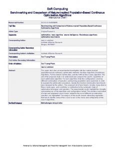
P| |T P | T P r = |T P|T|+|F N | = |P | (plotted on the Y -axis). A point (F P r, T P r) depicting rule R in the ROC space is determined by the covering properties of the rule. The ROC space is appropriate for measuring the success of subgroup discovery, since rules/subgroups whose T P r/F P r tradeoff is close to the diagonal can be discarded as insignificant; the reason is that the rules with T P r/F P r on the diagonal have the same distribution of covered positives and negatives as the distribution in the training set. Conversely, significant rules/subgroups are those sufficiently distant from the diagonal. Subgroups that are optimal under varying T P r/F P r tradeoffs form a convex hull called the ROC curve. Figure 2 presents seven rules on the convex hull (marked by circles), including X1 and X2, while two rules B1 and B2 below the convex hull (marked by +) are of lower quality in terms of their T P r/F P r tradeoff.

Fig. 2. The left-hand side figure shows the ROC space with a convex hull formed of seven rules that are optimal under varying T P r/F P r tradeoffs, and two suboptimal rules B1 and B2. The right-hand side presents the positions of the same rules in the corresponding T P/F P space.

It was shown in [16] that for rule R, the vertical distance from the (F P r, T P r) point to the ROC diagonal is proportional to the significance of the rule. Hence, the goal of a subgroup discovery algorithm is to find subgroups in the upperleft corner area of the ROC space, where the most significant rule would lie in point (0, 1) representing a rule covering only positive and none of the negative examples (F P r = 0 and T P r = 1).

Relevancy in Constraint-Based Subgroup Discovery

253

An alternative to the ROC space is the so-called T P/F P space (see the righthand side of Figure 2), where F P r on the X-axis is replaced by |F P | and T P r on the Y -axis by |T P |.7 The T P/F P space is equivalent to the ROC space when comparing the quality of subgroups induced in a single domain. The reminder of this paper considers only this simpler T P/F P space representation.

Interpretation of Relevancy in the T P /F P Space

4

The concept of feature coverage introduced in this section is important as a relevancy constraint used in rule learning. The concept is not valid only for features but also for conjunctions of features and for complete rules. Filtering based on absolute and relative relevancy introduced in this section can be applied in every domain. While the aim of absolute relevancy is to provide the minimal quality constraint required for every feature (rule), relative relevancy aims to ensure that only the best among available features will enter the rule construction process. The definition of relative irrelevancy is very useful because it does not depend on user-defined constraints. Relevancy-based filtering is therefore applicable in all feature-based machine learning applications [14]. It is useful also as a preprocessing filter for other symbolic learners such as decision tree learners, because complete attributes can be eliminated as irrelevant if all features generated for these attributes are detected as relatively or absolutely irrelevant. 4.1

Relative Relevancy

Let us now re-interpret the notions introduced in Sections 3.2 and 3.3 from the point of view of feature relevancy. Definition 4: Coverage of features (revisited Definition 3) Feature frel covers feature f (i.e., feature frel is more relevant than f ) iff true positives of f are a subset of true positives of frel and true negatives of f are a subset of true negatives of frel , i.e., iff T P (f ) ⊆ T P (frel ) and T N (f ) ⊆ T N (frel ) (see Figure 3). Definition 5: Relative relevancy Feature f is relatively irrelevant iff there exists another feature frel such that frel covers f . Theorem 1. If feature frel covers feature f and feature grel covers g then frel ∧ grel covers f ∧ g. 7

The T P/F P space can be turned into the ROC space by simply normalizing the T P and F P axes to the [0,1]x[0,1] scale.

254

N. Lavraˇc and D. Gamberger

Fig. 3. The concept of relative relevancy illustrated by features f and frel . Feature f is relatively irrelevant because T P (f ) ⊆ T P (frel ) and T N (f ) ⊆ T N (frel ).

It is trivial to prove this theorem by first fixing one of the two conjuncts grel = g and showing that T P (f ∧g) ⊆ T P (frel ∧g) and T N (f ∧g) ⊆ T N (frel ∧g). Next, the same relationship can be shown also for the case when grel covers g.8 

Relative relevancy of features is an important concept as feature f is not necessarily irrelevant because of its low |T P | or |T N | values but because there exists another more relevant feature with better covering properties. Therefore a relevancy filter using the concept of relative relevancy of features will never eliminate a feature that could potentially be relevant in conjunction with other features, as the more relevant feature which caused its elimination will take its role in the conjunction. Relative relevance ensures the quality of induced rules and, even more importantly from the point of view of avoiding overfitting, it ensures that rule learners will use only the best features available. Consider now the simplest form of rules, whose conditions consist of a single feature. Suppose such rules are plotted in the T P/F P space, meaning that each feature represents a point in the T P/F P space. The more distant a feature is from the diagonal, the more significant is the feature. ‘Good’ features are those as close as possible to point (0, P ) in T P/F P space. The left-hand side of Figure 4 presents the concept of relative relevancy. As |T P (f )| ≤ |T P (frel )|, feature 8

Theorem 1 can be proved also for the logical OR operation frel ∨grel . Consequently, if for feature f there exists another feature frel with the property that if in any rule f is substituted by frel the rule quality measured by the number of correct classifications |T P | and |T N | does not decrease, then frel can be always used instead of f , and feature f can be eliminated as irrelevant.

Relevancy in Constraint-Based Subgroup Discovery

255

Fig. 4. The left-hand side figure presents the concept of relative relevancy while the right-hand side figure presents the concept of absolute relevancy

frel is plotted higher along the T P -axis. As |T N (f )| ≤ |T N (frel )|, therefore |F P (frel )| ≤ |F P (f )|, and feature frel is plotted more to the left (closer to the T P -axis) along the F P -axis than feature f . Figure 4 shows feature f , a shaded area in the upper-left corner of f showing a part of the T P/F P space of features frel that are potentially more relevant than f , and a shaded area in the lower-right corner of frel showing the part of the space of features that are potentially irrelevant due to the existence of frel . Note that not all features left-up of f are more relevant and not all features right-down of frel are irrelevant, but only those that satisfy Definition 4. 4.2

Total Relevancy

In addition to irrelevant features defined through relative relevancy, also totally irrelevant features—those which are totally useless for distinguishing between the classes—can be eliminated in preprocessing. Definition 6: Total irrelevancy Feature f with |T P (f )| = 0 or |T N (f )| = 0 is totally irrelevant. 4.3

Absolute Relevancy

In order for a feature to be acceptable as a building block of rule conditions representing some genuine dependencies between classes and attribute values, the feature itself must have appropriate covering properties on the training set. These can be defined in terms of user-defined support constraints. Definition 7: Absolute irrelevancy Feature f that has either |T P (f )| < M inT P or |T N (f )| < M inT N is absolutely irrelevant, for M inT P and M inT N being user defined constraints. For low values of M inT P and M inT N , feature f with |T P (f )| < M inT P is true for a small number of target class examples, and feature g with |T N (g)| < M inT N is false for a small number of non-target class examples. Such small numbers may be due to statistical chance so that it seems reasonable not to

256

N. Lavraˇc and D. Gamberger

Fig. 5. The selection of the optimal M inT P constraint based on the properties of a previously detected good rule R

use features with either of these properties in the rule construction process. The part of the T P/F P space of absolutely irrelevant features is represented by the shaded area of the right-hand side figure of Figure 4. Although the significance of rules is proportional to their distance from the diagonal in the T P/F P space (Figure 2), this property is not appropriate as a quality criterion for features. As logical combinations of features lying on the diagonal or very near to it can result in very significant conjunctions of features (rules), only relative and absolute relevancy constraints defined in this work are considered as appropriate for feature filtering. By conjunctions of features, the generated rule will have |T P | equal or smaller than the smallest |T P | value of the features forming a conjunctive subgroup description. In contrast, the |T N | value of a rule will be at least as large as the largest |T N | of the used features. This is the reason why M inT P is typically selected higher than M inT N (see the right-hand side figure of Figure 4) and it can be as large as the minimal estimated number of examples that must be covered by a subgroup of acceptably high quality for the domain. The problem with absolute irrelevancy is that both M inT P and M inT N are user defined constraints and that any value, regardless how high it is, can not guarantee that a feature is actually relevant. A practical suggestion is to start with their low values of these constraints and after that to experiment with higher values. The optimal point is just before a significant decrease of covering properties of induced rules can be noticed. A good starting  values for gene expression domains are M inT P = |P |/2 and M inT N = |N | which have been used in all the experiments reported in Section 7. The selection of these constraints is not very critical for the final result because the majority of absolutely irrelevant features is detected also as relatively irrelevant. With mentioned M inT P and M inT N values in gene expression domains more than 90% of absolutely irrelevant features were detected as being also relatively irrelevant.

Relevancy in Constraint-Based Subgroup Discovery

4.4

257

Analysis of Absolute Relevancy Constraints in the T P/F P Space

The major problem of the concept of absolute relevancy is the selection of appropriate M inT P and M inT N constraints. In cases when rules are built exclusively as conjunctions of features (as in the SD algorithm), the problem can be at least partially solved by the analysis of the M inT P constraint in the T P/F P space. Let us suppose that in the process of rule construction rule R (that could be also a single feature) represents the best solution detected so far or that we are able to estimate its properties based on previous experiments in the domain. The position of rule R in the T P/F P space is determined by its T P (R) and F P (R) values. In Figure 5 the line drawn through this point presents the line connecting all the points in the T P/F P space that have the same rule quality qg as rule R. For various quality measures the slope of the line is different. For (R)| 9 the qg (R) measure used in the SD algorithm [7] the slope is equal to |F|TPP(R)|+g . This line cuts the T P axis in point A with value |F P (A)| = 0 and some positive value |T P (A)|. Setting M inT P = |T P (A)| is a good choice for the M inT P constant because any conjunctive combination with a feature which has |T P | value below |T P (A)| can, in an ideal case, lead to a rule lying below point A and therefore have a lower quality than the already detected rule R. For the qg (R) (R)| 10 measure this value is g · |F|TPP(R)|+g . It can be noted that a better intermediate rule R (with higher |T P (R)| and lower |F P (R)| values) enables the selection of a higher M inT P value, resulting in the elimination of more features and faster search without a decrease in the final rule quality. This property can be used so that the M inT P value is adjusted dynamically to the best detected solution so far. The result is feature relevancy detection during the rule construction process. For very time consuming algorithms it can be useful to first detect a good R by a fast heuristic search algorithm in advance before starting the main rule construction process, ensuring that relevancy filtering can be done before starting the rule construction process. The described analysis can not help us to estimate the optimal M inT N value. In cases when rules are built by disjunctive instead of conjunctive connections of features, analogous reasoning is valid, which helps to select good M inT N values but then M inT P should be estimated and selected by the user. 4.5

Relevancy of Rules

The defined relations of relative and absolute relevancy are valid not only for rules consisting of a single feature but they can be applied to any logical combination of features that can be constructed in the rule induction process, as well as to complete rules. This property is very important because it can significantly reduce the time and space complexity of learning algorithms. In the SD 9

10

For example, for the weighted relative accuracy measure, WRAcc [16], the slope of |P | the line equals |N| . When the WRAcc rule quality measure is used, the optimal M inT P value for rule |P | . R equals |T P (R)| − |F P (R)| · |N|

258

N. Lavraˇc and D. Gamberger

algorithm, the properties of relative and absolute relevancy are tested in each of its iterations for all the constructed conjunctive combinations of features. In SD, the M inT P absolute relevancy constraint is implemented by the user-defined M inSup constraint, while the M inT N constraint is ensured by setting the absolute relevancy threshold for all the generated features.

5

Using the Concept of Relevancy in Handling of Unknown Values

The concept of relevancy can be used in handling of unknown values based on the guideline that by the elimination/replacement of unknown values the relevancy of features should not increase. By following this guideline, the approach proposed in this section contributes to preventing data overfitting, especially in domains with a large number of unknown attribute values. The proposed approach is different from typical procedures for handling unknown values such as considering the unknown value as an additional regular value or substituting of the unknown value by the most common or by a proportional fractional value [4]. To ensure that unknown value handling will not increase feature relevancy, an attribute with an unknown value in a positive example is—in all features constructed from this attribute—replaced by value false, while an unknown value occurring in a negative example is replaced by value true in all features constructed from the same attribute. Table 2. Features generated from an attribute with value unknown (?) have value false if the example is positive, and value true if the example is negative. Feature values generated from unknown attribute values are presented in bold. Examples Attributes Ex. Cl. X Y X=A p1 ⊕ A 5 true p2 ⊕ ? 4 false p3 ⊕ P ? f alse n1  ? 2 true n2  A ? true n3  P 1 f alse

X = A f alse false true true f alse true

F eatures X = P X = P f alse true false false true f alse true true f alse true true f alse

Y >3 true true false f alse true f alse

Y ≤3 f alse f alse false true true true

Example 2. Consider a domain with three positive examples, three negative examples, two attributes (one discrete and one continuous-valued), four features generated for the discrete attribute, and two (out of possibly many) features for the attribute with continuous values. The domain is presented in Table 2. It can be noticed that for known attribute values a feature and its complement always have different truth values, but for unknown attribute values all features have the same value: false if the example is positive and true if the example is negative. 

Relevancy in Constraint-Based Subgroup Discovery

6

259

Using the Concept of Relevancy in Gene Expression Data Preprocessing

In some domains, like in the gene expression domain, there is a possibility to choose between different types of attributes and when confronted with this choice, the preference should be given to those leading to more relevant features. 6.1

Choice of the Language of Features

Gene expression scanners measure signal intensity as continuous values which form an appropriate input for data analysis. The problem is that for continuous valued attributes there can be potentially many boundary values separating the classes, resulting in many different features for a single attribute. There is also a possibility to use presence call (signal specificity) values computed from measured signal intensity values by the Affymetrix GENECHIP software. The presence call has discrete values A (absent), P (present), and M (marginal). Subgroup discovery as well as filtering based on feature and rule relevancy are applicable both for signal intensity and/or the presence call attribute values. Typically, signal intensity values are used [17] because they impose less restrictions on the classifier construction process and because the results do not depend on the GENECHIP software presence call computation. For subgroup discovery we prefer the later approach based on presence call values. The reason is that features presented by conditions like Gene = P is true (meaning that Gene is present, i.e., expressed) or Gene = A is true (meaning that Gene is absent, i.e., not expressed) are very natural for human interpretation and that the approach can help in avoiding overfitting, as the feature space is very strongly restricted, especially if the marginal value M is encoded as value unknown. 6.2

Handling Unknown Values and Feature Filtering

In the gene expression domain the M value is handled as an unknown value because we do not want to increase the relevance of features generated from attributes with M values. As for the other two values, A and P , it holds that two features for gene X, X = A and X = P , are identical (see Table 2). Consequently, for every gene X there are only two distinct features X = A and X = P . As suggested in Section 5, unknown values coming from marginal attribute values in positive examples are replaced by value false, while in negative examples they are replaced by value true. Example 3. The approach applied in gene expression data analysis is illustrated in Table 3. The table presents five positive and four negative examples for one of the target classes in the gene expression domain. Only features generated from presence call values of three attributes (genes) are presented. Observe that in this example, following Definition 5 of relative relevancy, feature X = A is relatively irrelevant because of feature Y = A, and feature X = P is relatively irrelevant because of feature Z = A. Consequently, both features generated for gene X can be eliminated as irrelevant. 

260

N. Lavraˇc and D. Gamberger

Table 3. Training examples represented as vectors of truthvalues of features. Notice that value M (marginal) is treated as an unknown attribute value. Examples Genes Ex. Cl. X Y Z p1 ⊕ A A A p2 ⊕ P P A p3 ⊕ A A P p4 ⊕ P P A p5 ⊕ M A A n1  A P P n2  P P P n3  M M A n4  P P A

7

X=A true f alse true f alse f alse true f alse true f alse

X=P f alse true f alse true f alse f alse true true true

F eatures Y =AY =P true f alse f alse true true f alse f alse true true f alse f alse true f alse true true true f alse true

Z=A true true f alse true true f alse f alse true true

Z=P f alse f alse true f alse f alse true true f alse f alse

Experiments in Functional Genomics

The gene expression domain, described in [25,8] is a domain with 14 different cancer classes and 144 training examples in total. Eleven classes have 8 examples each, two classes have 16 examples and only one has 24 examples. The examples are described by 16063 attributes presenting gene expression values. In all the experiments we have used gene presence call values (A, P , and M ) to describe the training examples. The domain can be downloaded from http://www-genome.wi.mit.edu/cgi-bin/cancer/datasets.cgi. There is also an independent test set with 54 examples. The standard goal of machine learning is to start from such labeled examples and construct classifiers that can successfully classify new, previously unseen examples. Such classifiers are important because they can be used for diagnostic purposes in medicine and because they can help to understand the dependencies between classes (diseases) and attributes (gene expressions values). The experiments were performed separately for each cancer class so that a two-class learning problem was formulated where the selected cancer class was the target class and the examples of all other classes formed non-target class examples. In this way the domain was transformed into 14 inductive learning problems, each with the total of 144 training examples and between 8 and 24 target class examples. For each of these tasks a complete procedure consisting of feature construction, elimination of irrelevant features, and induction of subgroup descriptions in the form of rules was repeated. Finally, using the SD subgroup discovery algorithm [7], for each class a single rule R with maximal | being the heuristic of the SD algoqg (R) value was selected, for qg (R) = |F|TPP|+g rithm and g = 5 as the generalization parameter default value. The rules for all 14 tasks consisted of 2–4 features. The procedure was repeated for all 14 tasks with the same default parameter values. The induced rules were tested on the independent example set. There are very large differences among the results on the test sets for various classes (diseases) and the precision higher than 50% was obtained for only 5 out

Relevancy in Constraint-Based Subgroup Discovery

261

of 14 classes. There are only three classes (lymphoma, leukemia, and CNS) with more than 8 training cases and all of them are among those with high precision on the test set, while for only two out of eleven classes with 8 training cases (colorectal and mesothelioma) high precision was achieved. The classification properties of rules induced for classes with 16 and 24 target class examples (lymphoma, leukemia and CNS) are comparable to those reported in [25] (see Table 4), while the results on eight small example sets with 8 target examples were poor. An obvious conclusion is that the use of the subgroup discovery algorithm is not appropriate for problems with a very small number of examples because overfitting can not be avoided in spite of the heuristics used in the SD algorithm and the additional domain-specific techniques used to restrict the hypothesis search space. But for larger training sets the subgroup discovery methodology enabled effective construction of relevant rules. Table 4. Covering properties on the training and on the independent test set for rules induced for three classes with 16 and 24 examples. Sensitivity is |T|PP|| , specificity is |T N| , |N|

while precision is defined as

|T P | . |T P |+|F P |

Cancer

Training set Sens. Spec. Prec. lymphoma 16/16 128/128 100% leukemia 23/24 120/120 100% CNS 16/16 128/128 100%

7.1

Test set Sens. Spec. Prec. 5/6 48/48 100% 4/6 47/48 80% 3/4 50/50 100%

Experiments in Feature Filtering

In the rest of this chapter experiments are performed on three classes with a sufficient number of training instances—lymphoma, leukemia, and CNS—for which induction of significant rules was possible. Table 5 shows the summary of results obtained by different experiments in eliminating irrelevant  features. For absolute relevance default values M inT P = |P |/2 and M inT N = |N | as proposed in Section 4.3 were used. Task 1. In the real domain with 16063 attributes both concepts of absolute and relative relevancy were very effective in reducing the number of features. About 60% of all features were detected as absolutely irrelevant while relative irrelevancy was even more effective as it managed to eliminate up to 75% of all the features. Their combination resulted in the elimination of 75%–85% of all the features. These results are presented in the first row of Table 5. The set of all features in these experiments was generated so that for each gene (attribute) two features were constructed (Gene = A and Gene = P ), followed by eliminating totally irrelevant features (with |T P | = 0 or |T N | = 0), which substantially reduced the total number of features.

262

N. Lavraˇc and D. Gamberger

Table 5. This table presents mean numbers of constructed features for the lymphoma, leukemia, and CNS domains. Presented are the total number of features (All), the number of features after the elimination of totally irrelevant features (Total), the number of features after the elimination of absolutely irrelevant features (Absolute), and the number of features after the elimination of absolutely and relatively irrelevant features (Relative). These three values are shown for the following training sets: the real training set with 16063 genes (with 32126 gene expression activity values, constructed as Gene = A and Gene = P ), a randomly generated set with 16063 genes, and a set with 32126 genes which is a combination of 16063 real and 16063 random attributes. Tasks All Task 1 Real domain with 16063 att. 32126 Task 2 Randomly generated domain with 16063 att. 32126 Task 3 Combination of 16063 real and 16063 randomly generated attributes 64252

Total

Absolute Relative

23500

9628

4445

27500

16722

16722

51000

26350

15712

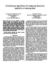
Task 2. Another domain with 16063 completely randomly generated attribute values was also constructed, and the same experiments were repeated on this artificial domain as for the real gene expression domain. The results (repeated with five different randomly generated attribute sets) were significantly different: there were only about 40% of absolutely irrelevant features and practically no relatively irrelevant features. The results are presented in the second row of Table 5. Comparing the results for the real and for the randomly generated domain, especially large differences can be noticed in the performance of relative relevancy. It is the consequence of the fact that in the real domain there are some features that are really relevant; they cover many target class examples and a few non-target class examples and in this way they make many other features relatively irrelevant. The results prove the importance of relative relevancy for domains in which strong and relevant dependencies between classes and attribute values exist. Task 3. The experiments with feature relevancy continued with another domain with 32126 attributes, generated as the combination of two previous domains with 16063 attributes each: the real and the randomly generated domain. The results are presented in the last row of Table 5. After the elimination of absolutely irrelevant features the number of features is equal to the sum of features that remained in the two independent domains with 16063 attributes. In contrast, relative relevancy was much more effective. Besides eliminating many features from the real attribute part it was now possible to eliminate also a significant part of features of randomly generated attributes. Summary of the experiments. Figure 6 illustrates the results presented in Table 5 with one added domain with 32126 randomly generated attributes. From

Relevancy in Constraint-Based Subgroup Discovery

263

Fig. 6. Mean numbers of features for the three domains (lymphoma, leukemia, and CNS) for the following training sets: real training set with 16063 attributes of gene expression activity values, a randomly generated set with 16063 attributes, a randomly generated set with 32126 attributes, and a set which is a combination of 16063 real and 16063 random attributes

this analysis it is obvious that the elimination of features is very effective in real domains. The same result were confirmed in experiments with domains with only 8 target class examples. It is important that in domains which are combinations of real and random attributes the proposed feature filtering methodology is effective: in Task 3 less features remained after feature elimination (15712 features) than in Task 2 (16722 features). This proves that the presented methodology, especially relative relevancy, can be very useful in avoiding overfitting by reducing the hypothesis search space through the elimination of non-significant dependencies between attribute values and classes. This property is important because it can be assumed that among 16063 real attributes there are many of them which are irrelevant with respect to the target class. 7.2

Examples of Induced Rules

For three classes (lymphoma, leukemia, and CNS) with more than 8 training cases the following rules were induced by the constraint-based subgroup discovery approach involving relevancy filtering and handling of unknown values described in this chapter. Lymphoma class: (CD20 receptor EXPRESSED) AND (phosphatidylinositol 3 kinase regulatory alpha subunitNOT EXPRESSED)

264

N. Lavraˇc and D. Gamberger

Leukemia class: (KIAA0128 gene EXPRESSED) AND (prostaglandin d2 synthase gene NOT EXPRESSED) CNS class: (fetus brain mRNA for membrane glycoprotein M6 EXPRESSED) AND (CRMP1 collapsin response mediator protein 1 EXPRESSED) The expert interpretation of the results yields several biological observations: two rules (for the lymphoma and leukemia classes) are judged as reassuring and one (the CNS class) has a plausible, albeit partially speculative explanation. Namely, the best-scoring rule for the lymphoma class in the multi-class cancer recognition problem contains a feature corresponding to a gene routinely used as a marker in diagnosis of lymphomas (CD20), while the other part of the conjunction (phosphatidylinositol, the PI3K gene) seems to be a plausible biological co-factor. The best-scoring rule for the leukemia class contains a gene whose relation to the disease is directly explicable (KIAA0128, Septin 6). Both M6 and CRMP1 appear to have multifunctional roles in shaping neuronal networks, and their function as survival (M6) and proliferation (CRMP1) signals may be relevant to growth promotion and CNS malignancy. Both good prediction results on an independent test set (Table 4) as well as expert interpretation of induced rules prove the effectiveness of described methods for avoiding overfitting in scientific discovery tasks.

8

Conclusions

This chapter reinterprets the theory of relevancy, described in [14,15], as relevancy constraints applied in a constraint-based subgroup discovery. Although the target is the induction of rules presenting subgroup descriptions, the results concerning the concept of relevancy are more general and valid for any feature-based rule learner. The chapter presents the theory of feature relevancy in the context of ROC analysis and provides an experimental evaluation of the usefulness of feature elimination in a functional genomics domain. We have implemented domain dependent restrictions by using discrete instead of continuous attribute values, and domain independent restrictions by the elimination of irrelevant features. Interpretation of marginal gene values as unknown values helped in reducing the feature space and ensured the robustness of induced rules. The proposed subgroup discovery framework proved to be useful for solving scientific discovery tasks.

Acknowledgments This work was supported by the Slovenian Ministry of Higher Education, Science and Technology, and the Croatian Ministry of Science, Education and Sport.

Relevancy in Constraint-Based Subgroup Discovery

265

References 1. H. Almuallim and T.G. Dietterich. Learning with many irrelevant features, In Proceedings of the 9th National Conference on Artificial Intelligence, The MIT Press, 547–552, 1991. 2. R.J. Bayardo, R.Agrawal, and D.Gunopulos. Constraint-based rule mining in large, dense databases. In Proc. of the 15th Conference on Data Engineering, 188-197, 1999. 3. R.J. Bayardo, editor. Constraints in Data Mining. Special issue of SIGKDD Explorations, 4(1), 2002. 4. I. Bruha and F. Franek. Comparison of various routines for unknown attribute value processing. Journal of Pattern Recognition and Artificial Intelligence 10(8): 939–955, 1996. 5. P. Clark and T. Niblett. The CN2 induction algorithm. Machine Learning, 3(4): 261–283, 1989. 6. U.M. Fayyad and K.B. Irani. On the handling of continuous-valued attributes in decision tree generation. Machine Learning 8: 87–102, 1992. 7. D. Gamberger and N. Lavraˇc. Expert-guided subgroup discovery: Methodology and application. Journal of Artificial Intelligence Research 17: 501–527, 2002. ˇ 8. D. Gamberger, N. Lavraˇc, F. Zelezn´ y, and J. Tolar. Induction of comprehensible models for gene expression datasets by the subgroup discovery methodology. Journal of Biomedical Informatics 37:269–284, 2004. 9. K. Kira and L.A. Rendell. A practical approach to feature selection, In Proceedings of the 9th International Conference on Machine Learning, Morgan Kaufmann, 249– 256, 1992. 10. W. Kl¨ osgen. Explora: A multipattern and multistrategy discovery assistant. In Advances in Knowledge Discovery and Data Mining, 249–271, MIT Press, 1996. 11. R. Kohavi and G.H. John. Wrappers for feature subset selection. Artificial Intelligence, Special Issue on Relevance, 97: 273-324, 1997. 12. D. Koller and M. Sahami. Toward optimal feature selection. Proceedings of the 13th International Conference on Machine Learning, Morgan Kaufmann, 284–292, 1996. 13. I. Kononenko. Estimating attributes: Analysis and extensions of Relief, In Proceedings of the 7th European Conference on Machine Learning, LNAI 784, Springer, 171–182, 1994. 14. N. Lavraˇc, D. Gamberger, and P. Turney. A relevancy filter for constructive induction. IEEE Intelligent Systems and their Applications 13: 50–56, 1998. 15. N. Lavraˇc, D. Gamberger and V. Jovanoski. A study of relevance for learning in deductive databases. Journal of Logic Programming 40: 215–249, 1999. 16. N. Lavraˇc, B. Kavˇsek, P. Flach and L. Todorovski. Subgroup discovery with CN2SD. Journal of Machine Learning Research, 5: 153–188, 2004. 17. J. Li and L. Wong. Geography of differences between two classes of data. In Proc. of 6th European Conference on Principles of Data Mining and Knowledge Discovery (PKDD2002), Springer, 325–337, 2002. 18. H. Liu and H. Motoda, editors. Feature Selection for Knowledge Discovery and Data Mining. Kluwer, 1998. 19. H. Mannila and H. Toivonen. Levelwise search and borders of theories in knowledge discovery. Data Mining and Knowledge Discovery, 1(3): 241–258, 1997. 20. R.S. Michalski. A theory and methodology of inductive learning, In: R. Michalski, J. Carbonell and T. Mitchell (eds.) Machine Learning: An Artificial Intelligence Approach, Tioga, 83–134, 1983.

266

N. Lavraˇc and D. Gamberger

21. S. Morishita and J. Sese. Traversing itemset lattices with statistical metric pruning. In Proceedings of the Nineteenth Symposium on Principles of Database Systems, 226–236, 2000. 22. A.L. Oliveira and A.Sangiovanni-Vincentelli. Constructive induction using a nongreedy strategy for feature selection. In Proceedings of the 9th International Conference on Machine Learning, Morgan Kaufmann, 354–360, 1992. 23. F. Provost and T. Fawcett. Robust classification for imprecise environments. Machine Learning, 42(3): 203–231, 2001. 24. J.R. Quinlan. C4.5: Programs for Machine Learning. Morgan Kaufmann, (1993). 25. S. Ramaswamy et al. Multiclass cancer diagnosis using tumor gene expression signatures. In Proc. Natl. Acad. Sci. USA, 98(26): 15149–15154, 2001. 26. S. Wrobel. An algorithm for multi-relational discovery of subgroups. In Proceedings of the 1st European Symposium on Principles of Data Mining and Knowledge Discovery, Springer, 78–87, 1997.