reliability-based optimization of layout and sizing of water distribution

Twelfth International Water Technology Conference, IWTC12 2008, Alexandria, Egypt

759

RELIABILITY-BASED OPTIMIZATION OF LAYOUT AND SIZING OF WATER DISTRIBUTION SYSTEMS Berge Djebedjian *, Ashraf Yaseen ** and Riham Ezzeldin *** *

Mechanical Power Engineering Department, Faculty of Engineering, Mansoura University, El-Mansoura 35516, Egypt E-mail: [email protected] ** Damietta Drinking Water Company, Damietta, Egypt E-mail: [email protected] *** Irrigation and Hydraulics Department, Faculty of Engineering, Mansoura University, El-Mansoura, Egypt E-mail: [email protected]

ABSTRACT The present study concerns of developing a procedure which takes into account both the network layout and size optimization of water distribution networks under a prespecified level of reliability. The approach links a genetic algorithm as the optimization tool, the Newton method as the hydraulic simulation solver with the chance constraint formulation which takes in account the uncertainty in the nodal demands. The method starts with a predefined layout which includes all possible links. The method was capable of designing a layout of predefined reliability, including treelike and looped networks. The proposed approach was illustrated by applying it to the two-loop network. Keywords: Genetic Algorithms, Optimization, Chance Constraint, Reliability, Water Distribution Systems

INTRODUCTION As a vital part of water supply systems, water distribution networks represent one of the largest infrastructure assets of industrial society. Simulation of hydraulic behavior within a pressurized, looped pipe network is a complex task, which effectively means solving a system of nonlinear equations. The solution process involves simultaneous consideration of the energy and continuity equations and the head loss function (Wood and Funk [1]). A number of different methods for solving the steady-state network hydraulics have been developed over the years, [2]. These methods play an important rule in layout, design, and operation of water distribution networks. The cost of operating a water distribution network may be substantial (due to maintenance, repair, water treatment, energy costs, etc.), but still one of the main costs is that of the pipelines themselves.

760

Twelfth International Water Technology Conference, IWTC12 2008, Alexandria, Egypt

In recent years a number of optimization techniques have been developed primarily for the cost-minimization aspect of network planning, although some reliability studies and stochastic modeling of demands have been attempted as reviewed by Walters and Cembrowicz [3]. The importance of obtaining the best network layout and the optimal pipe diameter for each pipe is emphasized by the fact that the decisions made during the layout and design phases will determine the ultimate operation costs. Since joint consideration of network layout design is extremely complex and since layout is largely restricted by the location of the roads, most authors studied the least cost optimization only under reliability such as Lansey et al. [4], Babayan et al. [5],[6] and Djebedjian et al. [7]. Rowel and Barnes [8] were the first to consider the joint problem of layout and size optimization for looped water distribution networks. They developed a two-level model in which a least-cost branched layout is first determined. The looping requirement is then provided by the inclusion of redundant pipes interconnecting the branches of the network. Morgan and Goulter [9] developed a model using two linked linear programs to solve for the least-cost solution of looped networks. In this model, one linear program solves for the layout, while the other determines the optimal pipe design. The looping constraint is enforced by requiring that every node is connected by at least two pipes, which does not explicitly guarantee the true redundancy required by the looped networks. Morgan and Goulter [10] presented a model based on a linear programming method linked to a network solver. The linear model designs pipe sizes, while the network solver balances flows and pressures. Within the linkage between these two steps is a means for removing uneconomical pipes from the network. The procedure was continued until no pipe can be removed from the network without undermining the looping of the network. Kessler et al. [11] and Cembrowicz [12] proposed models for the design of the layout geometry based on the inclusion or exclusion of the links chosen from a predefined base graph. The previous literature reviews assume that pipe network optimization can be reduced to two separate optimization problems, in which the layout optimization is followed by a pipe size optimization. The aforementioned assumption is weak because of strong coupling between pipe sizing and layout determination for pipe networks. Walters and Lohbeck [13] proposed two genetic algorithms (GAs) using binary and integer coding for layout determination of tree-like networks and compared their storage and computational time requirements with dynamic programming.

Twelfth International Water Technology Conference, IWTC12 2008, Alexandria, Egypt

761

Davidson [14] was the first to address the layout optimization of looped networks. Emphasizing the need for joint optimization of layout and pipe sizing, he restricted his research to layout determination, due to the difficulty in selecting optimal component sizes, while maintaining a sufficient level of reliability. An evolution program was devised, incorporating the concept of the preference and threshold method into the conventional GA. The preference and threshold method (Davidson [14]) was used in the initial population generation, crossover and mutation stage of the process to ensure the feasibility of the networks. The complexity feature in the development of an algorithm capable of addressing this subject is the strong coupling between the layout and pipe size determination. On the other hand, the layout determination of pipe networks is much dependent on reliability considerations. Afshar [15] applied the max-min ant system (MMAS) to simultaneous layout and size optimization of pipe networks with a given reliability. A Deterministic concept of reliability was used in which the number of independent paths from the source node to the demand nodes was taken as the measure of the reliability. The formulation of the pipe network optimization with fixed layout was extended by relaxing the availability constraint of the problem and including a reliability constraint to be used for joint layout and pipe size optimization. Each link of the base graph was considered as the decision point of the problem. Afshar [16] presented a GA incorporating different selection algorithms for the simultaneous layout and pipe size optimization of water distribution networks. An engineering concept of reliability was used, in which the number of independent paths from source nodes to each of the demand nodes was considered as a measure of reliability. The method starts with a predefined layout, which includes all possible links. The method was capable of designing a layout of predefined reliability, including tree-like and looped networks. It was shown that a layout optimization of a network, followed by size optimization, didn’t lead to an optimal or a near optimal solution. This emphasizes the need for simultaneous layout and size optimization of networks, if an optimal solution is desired. He tested the method on two benchmark examples. The objective of this paper is to develop a procedure which takes into consideration both the network layout and the pipe size of a water branched network to obtain the least cost. Two stages are considered in the present study. In the first stage, the optimization of network layout and pipe size to find the least cost is obtained for different layout alternatives. In the second stage, the reliability-based optimization of network layout and pipe size to find the least cost is achieved according to the chance constraint formulation.

762

Twelfth International Water Technology Conference, IWTC12 2008, Alexandria, Egypt

MATHEMATICAL FORMULATION The chance constraint model is considered to be a stochastic model by considering that the future demand, Q j , is uncertain because of the unknown future conditions of the system. In order to solve this method, the cumulative probability distribution concept is applied by considering the future demand as an normal random variable with mean, µ Q , and standard deviation, σ Q , as: Q = N ( µ Q , σ Q ) . The mathematical formulation is completely explained in Djebedjian et al. [7] and Ezzeldin [17]; the following summarized the main equations. The coefficient of variation (COV) is written as:

COV = σ Q µ Q

(1)

The model can be expressed by the following objective function: Minimum Cost = min. i , j∈M

f (Di , j )

(2)

Subject to the constraints:

Dmin ≤ Di , j ≤ Dmax

µW j σWj

(3)

≤ φ −1 (1 − α j )

(4)

where α j is the probability level, µW j and σ W j are the mean and standard deviation determined from:

µW j =

K C i, j

j

σWj =

j

Hi − H j

K Ci, j

0.54

Li , j

Hi − H j Li , j

Di2,.j63 − µ Q j

(5) 1/ 2

0.54

Di2,.j63 + σ Q2 j

(6)

The head loss in the pipe, h f , is expressed by the Hazen-Williams formula:

hf =

K Ci, j

1.852

Li , j qi , j Di , j

1.852

4.8704

= Hi − H j

(7)

Twelfth International Water Technology Conference, IWTC12 2008, Alexandria, Egypt

763

where K is a conversion factor which accounts for the system of units used, (K = 10.6744 for qi , j in m3/s and Di , j and Li , j in m), C i , j is the Hazen-Williams roughness coefficient for the pipe connecting nodes i, j, Li , j is the length of the pipe connecting nodes i, j, and H i , H j are the pressure heads at nodes i, j.

GAMC_OLS Program The GAMC_OLS program has been written in FORTRAN and it is the extension of GAMCnet program used in Djebedjian et al. [7] and Yaseen [18]. The layout feasibility checking was added to GAMCnet program to take into consideration the feasibility of the new layout. The main idea of the program is producing new layout by deleting pipes, the number of deleted pipes are arbitrary. Best optimization is achieved by beginning the deletion of one pipe and increasing it to the maximum pipes that gives the tree presentation, i.e. without separation of nodes or sources. The deleted pipes numbers are selected randomly and multiprocessing are done for checking the feasibility of the new network layout. The main techniques used in the GAMC_OLS program are, Figure 1: 1- Producing new layouts by deleting pipes. 2- Layout feasibility to check the feasibility of the modified layout of network, i.e. the connectivity of all nodes and pipes to the original network. 3- Exclude repeated layouts. 4- Genetic algorithm technique to search for the optimal diameters. The source code of GA was developed by Carroll [19] and was used in the program after minor modifications. 5- Newton method for the hydraulic simulation of pipe network. The H-equations solution method (Larock et al. [20]) was used in the program. 6- Chance constraint formulation for the uncertainties and node and network reliabilities. In this study, the micro-Genetic Algorithm (µ GA), Krishnakumar [21], which is a "small population" GA is used. In contrast to the Simple Genetic Algorithm, which requires a large number of individuals in each population (i.e., 30 - 200); the µ GA uses a small population size. For the studied case, the µGA parameter values were: population size of 12 and crossover rate was set to 0.5 (uniform crossover). Different initial random number seeds were tested to find the optimal solution

764

Twelfth International Water Technology Conference, IWTC12 2008, Alexandria, Egypt Input Given Network

Input Required number of Deleted Pipes

Producing all Possible Alternative Layouts

Produce Optimized Diam eters for each Alternative Layout

Newton Simulation

Convert Optimized Diameters to Comm ercial Diameters

Analyze Given Network Get Pressure Heads & Velocities

No

M aximum Generation

Fitness

M aterial Cost

Yes

Penalty Cost

No

If : H ≥ H min V min ≤ V ≤ V max

Yes Comprise between produced groups of diameters to select the group that has the lower diameters cost

Best Solution for each Alternative Layout individually

Comprise between all Possible Alternative Layouts to select the Layout that has the lower cost

Output Best Alternative Layout

Figure 1. Flow chart for reliability-based optimization for sizing and layout

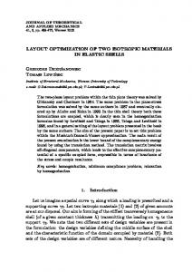
Case Study: Two-Loop Network The case study is a gravity fed two-loop network with 8 pipes, 7 nodes and one constant head reservoir. The layout of the network, the lengths of pipes and the node data are shown in Fig. 2. The two-loop network problem is originally presented by Alperovits and Shamir [22] and taken as a model network by many researchers, e.g. [23], [24]. All the pipes are 1000 m long and the Hazen-Williams coefficient is assumed to be 130 for all the pipes. The demands are given in cubic meters per hour and the minimum acceptable pressure requirement for each node is 30 m above the ground level. There are 14 commercially available pipe diameters and Table 1 presents the total cost (in arbitrary units) per meter of pipe length for different pipe sizes.

Twelfth International Water Technology Conference, IWTC12 2008, Alexandria, Egypt 210 m 100 m3/h

100 m3/h (150 m)

2

3

L = 1000 m

(160 m)

2

7

4

5

4 (155 m)

8

5

L = 1000 m

200 m3/h

(160 m)

L = 1000 m

330 m3/h

7

1

L = 1000 m

L = 1000 m

(150 m)

L = 1000 m

3

L = 1000 m 120 m3/h

270 m3/h

1

6 L = 1000 m

6 (165 m)

765

Table 1. Cost data for the two-loop network Diameter (inches) 1 2 3 4 6 8 10 12 14 16 18 20 22 24

Cost (units) 2 5 8 11 16 23 32 50 60 90 130 170 300 550

Figure 2. The two-loop network, Alperovits and Shamir [22]

Optimization of Layout and Sizing The different network layouts and associated cost can be studied depending on the water source or sources in the network. The original layout of the two-loop network has a single source and any modification in the layout should not have any change on the delivery of water to all nodes, i.e. all nodes stay in function after this modification. In this study the layout is modified by one of the following methods: 1)

Optimization of the network when the basic layout of the system is not given, i.e. the demands at nodes 2 to 7 are given and the optimal layout that gives the least construction cost under minimum nodal heads requirements is searched. The approach is to seek systematic method for automatically generating the optimized layout. The maximum possible shortest paths between these six nodes are illustrated in Fig. 3. It is assumed that there are no constructing restrictions in the region. The new network has 12 pipes and the optimization was done for different layouts by deleting 1 to six pipes from the proposed network.

766

Twelfth International Water Technology Conference, IWTC12 2008, Alexandria, Egypt 210 m

2

3

9

7

1

2

1

3 10

4

5

4 11

8

5 12

7

6

6

Figure 3. The two-loop network with all additional pipes

2)

Optimization of the network when the basic layout is given, Fig. 2, i.e. engineers have developed the layout with a measure of experience. Therefore, the network is restricted with the given paths between nodes. This network was tested by many researchers and the optimal cost is 419,000 units, e.g. [7]. However, one can delete one or two pipes from the original layout. It is well-known that for each loop, one of the pipes can be deleted without any change on the delivery of water to all nodes. For the two-loop network, the deletion of 1 pipe from each loop is done to constitute tree presentation. The total number of trees for the twoloop is 15.

Reliability-Based Optimization of Layout and Sizing The reliability-based optimization of layout and sizing when the basic layout is given, i.e. the previous second method, is studied. The chance constraint formulation for the uncertainties and node reliabilities is used as the reliability method. The chanceconstraint GA was used, allowing a reliability target to be considered. Two coefficients of variation (COV) equal 10% and 20% of nodal demand are used in the calculations. For each COV, a least-cost strategy with target reliabilities (uncertainty of the future demand) α j = 50, 60, 70, 80, 90 and 99% were created. A standard deviation equal to zero refers to the case of no uncertainty, and the larger the standard deviation, the greater the uncertainty. Using α = 0.5 is equivalent to using mean values of the nodal demands, i.e. optimization. Higher values of α refer to more stringent performance requirements so that the likelihood of not meeting future demands is reduced.

Twelfth International Water Technology Conference, IWTC12 2008, Alexandria, Egypt

767

RESULTS AND DISCUSSION The two previous mentioned alternatives for the layout optimization of the two-loop network were tested using the GAMC_OLS program which is based on genetic algorithm method. The optimization with GAMC_OLS allows a better representation of the system layout. The numerical computations made with GAMC_OLS solve the network layout selection, hydraulic analysis of network, the optimization and the reliability-based of network layout and sizing.

1. Optimization of Layout and Sizing for the Twelve Pipes Network The results obtained from optimization with GAMC_OLS program are compared in Table 1 for the new modified layout (12 pipes) and six alternative layouts (deleting 1 to 6 pipes). This is the maximum number of pipes that can be deleted without isolation of nodes and source. The number of layouts searched by the program, the optimal diameters and the optimal cost for each layout alternative are given in the table. The results reveal that the optimal cost for each alternative is lower than the optimal solution of the twelve pipes network shown in Figure 3 which is 407,152 units. It is worth to mention that the minimum cost for the six alternatives is the network modified by deleting six pipes which is 389,840 units using the mentioned optimal diameters. Also, for the twelve pipes network and the other layouts, there are many pipes with small diameter (1 inch) and deleting the pipes are practically preferred. From Table 2, it is revealed that increasing the number of deleted pipes from the network, the 1 inch diameter is disappeared from the optimal solution. Also, for Layout 3, there are two sets of diameters that fulfill the nodal pressure requirements and have the same cost. Figure 4 illustrates the relationship between the cost and number of deleted pipes from the twelve pipes network. There is a decrease in the optimal cost by decreasing the number of network pipes. The best solutions for Layout 1 to Layout 6 are shown in Figure 5. The pipes in layout 6 seem to play an important role in achieving the required nodal demands at restricted minimal nodal head as they exist in all other layouts. Also, layout 6 is the tree presentation (using minimum number of pipes) for the given number of nodes.

768

Twelfth International Water Technology Conference, IWTC12 2008, Alexandria, Egypt

Table 2. Comparison of the results of optimization for layout and size optimization for the twelve pipes network Layout Alternative

Number of Layouts

1

2

3

4

5

6

7

8

9

Modified Layout (12 pipes)

--

18

8

16

1

14

1

1

1

10 10

1

1

407,152

Layout 1 (Deleting 1 Pipe)

12

18

8

16

1

14

1

1

1

10 10

1

-

404,324

Layout 2 (Deleting 2 Pipes)

56

18

8

14

1

14

1

-

10 14

2

-

1

403,738

Layout 3 (Deleting 3 Pipes)

161

18

8

14

1

14

-

-

10 14

1

1

-

18

8

14

-

14

1

-

10 14

1

1

-

Layout 4 (Deleting 4 Pipes)

286

18

8

14

-

14

-

-

10 14

1

-

1

395,496

Layout 5 (Deleting 5 Pipes)

303

18

8

14

-

14

-

2

10 14

-

-

-

394,840

Layout 6 (Deleting 6 Pipes) - Tree Presentation

177

18

8

14

-

14

-

-

10 14

-

-

-

389,840

Diameters of pipes (inches) 10 11 12

420000

Cost (Units)

410000

400000

390000

380000

0

1

2

3

4

5

6

No. of deleted pipes

Figure 4. Optimal cost variation with number of deleted pipes from the twelve pipes network

Cost (units)

397,496

769

Twelfth International Water Technology Conference, IWTC12 2008, Alexandria, Egypt

210 m

2

3

9

7

1

2

1

210 m

2

3

9

3 10

4

5

1

2

3

9

3

4

5

4

1

3 10

4

5

4

8

5

1

2

10

11

8

1

2

210 m

11

8

5

4 5

12 6

7

6

7

6

Best Solution of Layout (1)

7

6

Best Solution of Layout (2) 210 m

2

3

1

2 9

2 9

3

5

4

6

7

1

7

6

11

1

2 9

1

3

6

Best Solution of Layout (4)

1

4 5

6

Best Solution of Layout (6)

Figure 5. Best solutions for Layouts 1 to 6

4 8

5

3

8

7

1

2 9

5

7

5

210 m

2

2

3

3

4 8

5

Best Solution of Layout (3) - B

3

210 m

10

11

8

1

2

10 5

Best Solution of Layout (3) - A 210 m

3

1

6

7

5

6

Best Solution of Layout (5)

770

Twelfth International Water Technology Conference, IWTC12 2008, Alexandria, Egypt

2. Optimization of Layout and Sizing for the Original Two-Loop Network The results obtained from optimization with GAMC_OLS program are compared in Table 3 for the best solutions of the two possible layout alternatives. Table 3 reveals that for each layout alternative there is at least one optimal solution with a cost less than that of the original network (419,000 units). The least cost of the two alternatives is achieved by deleting one pipe is (417,000 units) or two pipes (416,000 units). It can be concluded that in some cases as the studied one, the layout and sizing optimization has an important role in decreasing the total cost. However, it is worth to note that such network should be reliable and its reliability is the important factor for selection of a network. The optimal diameters given in Table 3 fulfill the requirements of minimum nodal head of 30 m. For Layout 7, there are 7 optimal feasible layouts while for Layout 8, there are 15 different optimal layouts depending on the number of deleted pipes. Table 3. Comparison of the results of optimization for layout and size optimization for the original two-loop network Layout Alternative

Layout 7 (Deleting 1 Pipe)

Layout 8 (Deleting 2 Pipes) Tree Presentation

Deleted Pipes Pipe 2 Pipe 3 Pipe 4 Pipe 5 Pipe 6 Pipe 7 Pipe 8 Pipes 2, 4 Pipes 2, 5 Pipes 2, 6 Pipes 2, 8 Pipes 3, 4 Pipes 3, 5 Pipes 3, 6 Pipes 3, 8 Pipes 4, 5 Pipes 4, 6 Pipes 4, 7 Pipes 4, 8 Pipes 5, 7 Pipes 6, 7 Pipes 7, 8

1

2

3

4

5

6

7

8

Cost (units)

20 20

20

18 -

14 12

14 10

4 14

8 20

10 14

486,000 712,000

20 20 18 18 18 20 20 18 20 20 20 20 20 20 18 18 20 20 18 18

10 16 14 8 10 20 20 20 20 20 14 8 10 8 8 8

16 14 14 18 16 20 20 18 18 8 14 20 16 20 18 18

16 1 10 4 20 16 12 8 16 18 18 14 10

14 14 16 16 18 14 16 8 14 18 14 18 14 14 16

10 16 10 10 16 16 10 16 16 10 16 14 10 16 10

10 14 14 10 10 8 8 8 20 20 20 20 18 14 10 -

1 16 12 1 14 16 12 18 16 10 16 12 10 16 12 -

418,000 650,000 422,000 439,000 417,000 652,000 713,000 483,000 495,000 753,000 713,000 692,000 802,000 673,000 420,000 545,000 416,000 673,000 453,000 437,000

Diameters of pipes (inches)

Similar to the previous presentation of best solutions for Layouts 1 to 6, Figure 6 shows the best solutions for Layouts 7 and 8. It can be noticed that for these two

Twelfth International Water Technology Conference, IWTC12 2008, Alexandria, Egypt

771

layouts, pipe 8, which provides water to node 7 the far node from the source, is deleted in the two networks. It reveals that its deleting is essential to obtain the optimal solution for the two layouts. 210 m

210 m

2

3 7

5

1

2

1

4

5

7

6

6

Best solution of Layout (7)

1

3

5

4

1

2

7

3 4

2

3

5

7

6

6

Best solution of Layout (8)

Figure 6. Best solutions for Layouts 7 and 8

3. Reliability-Based Optimization of Layout and Sizing The reliability-based optimization of layout and sizing for the deleting of one pipe (Layout 7) and two pipes (Layout 8) from the two-loop network was achieved using the GAMC_OLS program. The optimal cost and the pipe diameters of best solutions for different reliabilities α when the coefficients of variation (COV) are 10% and 20% of nodal demand for the original, Layout 7 and Layout 8 are summarized in Tables 4, 5 and 6, respectively, in the Appendix. Figure 7 shows the relationship between the cost and network reliability at coefficient of variation COV = 10% and COV = 20% for Layout 7. It is evident that at constant coefficient of variation, the cost increases with the increase of required network reliability. Also, for the same required reliability, the cost increases with the increase of coefficient of variation. This is expected due to the fact that the higher the reliability requirement, the greater the cost of design. The high reliability of network increases the performance of network at normal conditions. Figure 8 illustrates these results of cost and network reliability at coefficients of variation 10% and 20% for Layout 8 (15 cases). Generally, the cost increases with the increase of required network reliability and for the same required reliability, the cost increases with the increase of coefficient of variation. The coincidence of the two curves COV = 10% and COV = 20% at α = 0.5 reveals that the program performs optimization only. This is attributed to the fact that the nodal demands are the mean values without any variation. The value at this point for each of the 15 cases is the optimal cost given in Table 3 for the optimization. The verification of the effectiveness of reliability-based optimization for layout and sizing is achieved by getting the new layout that has cost less than the original layout

772

Twelfth International Water Technology Conference, IWTC12 2008, Alexandria, Egypt

(Figure 2) after optimization of sizing only, and both layouts (original and new) have the same certain degree of reliability. The least costs for the original layout and Layouts 7 and 8 obtained in Tables 4, 5 and 6, respectively, are given in Table 7 for the clarity of presentation. The best solution for the reliability-based optimization for Layout 7 requires the comparison between the costs for the two values of COV and five values of α for the 7 existing layout cases. Table 7 indicates that three layouts could achieve least cost compared with other producing layouts for different degrees of reliability. These layouts are resulted by deleting pipe 4, 6 or 8. For different COV and α, the results of deleting pipe 4 give 60% of the least costs. Therefore, it is chosen as the best solution for Layout 7. The comparison between the results of Layout 7 by deleting pipe 4 and that of the original two-loop network, Table 7, reveals that for each value of degree of reliability (except α = 0.99), there is a set of diameters that its cost is less than that of the original network. Generally, for all COV and α, there is at least one solution obtained by Layout 7 (deleting pipe 4, 8 or 6) is less than that of the original network. 1600000 Deleted Pipe 3, COV = 20% Deleted Pipe 3, COV = 10% Deleted Pipe 2, COV = 20% Deleted Pipe 2, COV = 10%

1200000

Cost (Units)

Cost (Units)

1600000

800000

400000 0.5

0.6

0.7

0.8

0.9

1

α

Deleted Pipe 5, COV = 20% Deleted Pipe 5, COV = 10% Deleted Pipe 7, COV = 20% Deleted Pipe 7, COV = 10%

1200000

800000

400000 0.5

0.6

0.7

0.8

0.9

α

(a) Deleted Pipe 2 and Pipe 3

(b) Deleted Pipe 6 and Pipe 7

800000

Cost (Units)

COV = 20% COV = 10%

Deleted Pipe 4

400000

Deleted Pipe 6 400000 Deleted Pipe 8

400000 0.5

0.6

0.7

0.8

0.9

1

α

(c) Deleted Pipe 4, Pipe 6 and Pipe 8

Figure 7. Total cost of network versus reliability α for COV = 10% and 20% (Layout 7)

1

Twelfth International Water Technology Conference, IWTC12 2008, Alexandria, Egypt

1200000

1600000 Deleted Pipes 2 and 4, COV = 20% Deleted Pipes 2 and 4, COV = 10% Deleted Pipes 2 and 6, COV = 20% Deleted Pipes 2 and 6, COV = 10%

Cost (Units)

Cost (Units)

1600000

800000

400000 0.5

0.6

0.7

0.8

0.9

1200000

800000

400000 0.5

1

Deleted Pipes 2 and 5, COV = 20% Deleted Pipes 2 and 5, COV = 10% Deleted Pipes 2 and 8, COV = 20% Deleted Pipes 2 and 8, COV = 10%

0.6

0.7

α

(b) Deleted Pipes 2 and 5, and Pipes 2 and 8 2000000

Deleted Pipes 3 and 4, COV = 20% Deleted Pipes 3 and 4, COV = 10% Deleted Pipes 4 and 7, COV = 20% Deleted Pipes 4 and 7, COV = 10%

1600000

Cost (Units)

Cost (Units)

0.9

2000000

1200000

800000

400000 0.5

1200000

800000

0.6

0.7

0.8

0.9

400000 0.5

1

0.6

0.7

0.8

0.9

(c) Deleted Pipes 3 and 4, and Pipes 4 and 7

(d) Deleted Pipes 3 and 8, and Pipes 7 and 8 1600000 Deleted Pipes 3 and 5, COV = 20% Deleted Pipes 3 and 5, COV = 10%

Cost (Units)

Deleted Pipes 5 and 7, COV = 20% Deleted Pipes 5 and 7, COV = 10% Deleted Pipes 6 and 7, COV = 20% Deleted Pipes 6 and 7, COV = 10%

800000

400000 0.5

0.6

0.7

0.8

0.9

1200000

800000

400000 0.5

1

0.6

0.7

α

(e) Deleted Pipes 5 and 7, and Pipes 6 and 7

0.9

1

0.9

1

(f) Deleted Pipes 3 and 5 1600000

Cost (Units)

Deleted Pipes 4 and 5, COV = 20% Deleted Pipes 4 and 5, COV = 10% Deleted Pipes 4 and 6, COV = 20% Deleted Pipes 4 and 6, COV = 10%

800000

400000 0.5

0.8

α

1600000

1200000

1

α

1600000

1200000

1

Deleted Pipes 3 and 8, COV = 20% Deleted Pipes 3 and 8, COV = 10% Deleted Pipes 7 and 8, COV = 20% Deleted Pipes 7 and 8, COV = 10%

α

Cost (Units)

0.8

α

(a) Deleted Pipes 2 and 4, and Pipes 2 and 6

1600000

Cost (Units)

773

0.6

0.7

0.8

0.9

α

(g) Deleted Pipes 4 and 5, and Pipes 4 and 6

1

1200000

Deleted Pipes 3 and 6, COV = 20% Deleted Pipes 3 and 6, COV = 10% Deleted Pipes 4 and 8, COV = 20% Deleted Pipes 4 and 8, COV = 10%

800000

400000 0.5

0.6

0.7

0.8

α

(h) Deleted Pipes 3 and 6, and Pipes 4 and 8

Figure 8. Total cost of network versus reliability α for COV = 10% and 20% (Layout 8)

774

Twelfth International Water Technology Conference, IWTC12 2008, Alexandria, Egypt

The seek for the best solution for the reliability-based optimization for Layout 8 is done by the comparison of the optimal costs for the 15 existing layout cases for the values of COV and α. Table 7 indicates that the two cases; deleting the two pipes 4 and 6 or 4 and 8; could achieve least cost compared with other cases for different COV and α. The results of deleting pipes 4 and 6 give 70% of the least costs obtained for different COV and α. Therefore, the best solution for Layout 8 is by deleting pipes 4 and 6. The network layout by deleting pipes 4 and 8 give 40% of the least costs obtained for different COV and α. Similar to the previous comparison between the results of the original two-loop network and Layout 8 by deleting pipes 4 and 6, Table 7 indicates that for high degrees of reliability (α = 0.9, 0.99), there is a set of diameters of the original network that its cost is less than that of Layout 8. For low degrees of reliability, the results obtained for Layout 8 have least costs less than that of the original network. On the other hand, for Layout 8 with deleting pipes 4 and 8, Table 7 shows that for tested values of COV and α greater than 0.6, the least cost of the set of diameters of the original network is less than that of the case of deleting pipes 4 and 8. Figure 9 illustrates the comparison between the least costs obtained for the original networks and Layouts 7 and 8. As mentioned before, for higher values of α, the results of the original network is less than that for Layouts 7 and 8 for both of COV = 10% and 20%. The difference increases with Layout 8 showing that tree presentations are not reliable at high degree of reliability. However, for α up to 0.8, the least costs of Layout 7 are generally less than that of the original network. On the other hand, Layout 8 results show discrepancies compared with the least cost of the original network confirming the reliability of tree presentations of networks. 550000

650000

500000

COV = 20%

Original Layout 7 Layout 8

600000

Cost (Units)

Cost (Units)

COV = 10%

450000

Original Layout 7 Layout 8

550000

500000

450000

400000 0.5

0.6

0.7

0.8

α

(a) COV = 10%

0.9

1

400000 0.5

0.6

0.7

0.8

0.9

α

(b) COV = 20%

Figure 9. Least cost of network versus reliability α for the original network, Layout 7 and Layout 8

1

Twelfth International Water Technology Conference, IWTC12 2008, Alexandria, Egypt

775

CONCLUSIONS Reliability-based optimization of layout and sizing of water distribution systems was presented. The genetic algorithms, chance constraint formulation, hydraulic simulation and layout feasibility were used in the approach. A computer program was developed and written in FORTRAN for the optimization and reliability-based optimization of layout and sizing. In the first part of study, the optimizations of the network when the layout of the system is not given or given are studied. For the undefined layout, the maximum possible shortest paths between the nodes are included to define the maximum layout and the optimization is achieved by decreasing the number of pipes used in the layout till having the tree presentation. For the defined basic layout, the same technique of decreasing the number of pipes is used. In the second part of study, the reliability-based optimization of layout and sizing was applied; the results reveal that at constant coefficient of variation, the cost increases with the increase of required network reliability. Also, for the same required reliability, the cost increases with the increase of coefficient of variation. This is expected due to the fact that the higher the reliability requirement, the greater the cost of design. The high reliability of network increases the performance of network at normal conditions. Generally, for all COV and α, there is at least one solution obtained by Layout 7 (deleting pipe 4, 8 or 6) is less than that of the original network. While for Layout 8, there are two cases (deleting the two pipes 4 and 6 or 4 and 8) could achieve least cost compared with other cases for different COV and α. For the Layout 8 and deleting pipes 4 and 6, there is a set of diameters of the original network that its cost is less than that of Layout 8 for high degrees of reliability (α = 0.9 and 0.99). For low degrees of reliability, the results obtained for Layout 8 have least costs less than that of the original network. For higher values of α, the results of the original network is less than that for Layouts 7 and 8 for both of COV = 10% and 20%. The difference increases with Layout 8 showing that tree presentations are not reliable at high degree of reliability. However, for α values up to 0.8, the least costs of Layout 7 are generally less than that of the original network. On the other hand, Layout 8 results show discrepancies compared with the least cost of the original network confirming the reliability of tree presentations of networks.

REFERENCES [1]

[2]

Wood, D.J., and Funk, J.E., "Hydraulic Analysis of Water Distribution Systems," in Water Supply Systems, State of the Art and Future Trends, E. Cabrera and F. Martinez, eds., Computational Mechanics Publications, Southampton, pp. 41-85 (1993). Bhave, P.R., and Gupta, R., Analysis of Water Distribution Networks, Alpha Science International Ltd., Oxford, U.K., 2006, 515 p.

776

Twelfth International Water Technology Conference, IWTC12 2008, Alexandria, Egypt

[3]

Walters, G.A., and Cembrowicz, R.G., "Optimal Design of Water Distribution Networks," Water Supply Systems, State of the Art and Future Trends, E. Cabrera and F. Martinez, eds., Computational Mechanics publications, Southampton, 1993, pp. 91-117. Lansey, K.E., Duan, N., Mays, L.W., and Tung, Y-K., "Water Distribution System Design under Uncertainties," Journal of Water Resources Planning and Management, ASCE, Vol. 115, No. 5, 1989, pp. 630-645. Babayan, A.V., Kapelan, Z., Savi , D.A., and Walters, G.A., "Least Cost Design of Robust Water Distribution Networks under Demand Uncertainty". Journal of Water Resources Planning and Management, ASCE, Vol. 131, No. 5, 2005, pp. 375-382. Babayan, A.V, Kapelan, Z., Savi , D.A., and Walters, G.A., "Comparison of Two Methods for the Stochastic least Cost Design of Water Distribution Systems," Engineering Optimization, Vol. 38, No. 3, April 2006, pp. 281-297. Djebedjian, B., Abdel-Gawad, H.A.A., Ezzeldin, R., Yaseen, A., and Rayan, M.A., "Evaluation of Capacity Reliability-Based and Uncertainty-Based Optimization of Water Distribution Systems," The Proceeding of the Eleventh International Water Technology Conference, IWTC 2007, March 15-18, 2007, Sharm El-Sheikh, Egypt, pp. 565-587. http://www.iwtc.info/2007/7-4.pdf Rowel, W.F. and Barnes, J.W., "Obtaining Layout of Water Distribution Systems", Journal of the Hydraulics Division, ASCE, Vol. 108, 1982, pp. 137148. Morgan, D.R. and Goulter, I.C., "Least cost layout and design of looped water distribution systems", in Proc. of Ninth Int. Symp. on Urban Hydrology, Hydraulics and Sediment Control, University of Kentucky, Lexington, KY, USA July 27-30, 1982. Morgan, D.R. and Goulter, I.C., "Optimal Urban Water Distribution Design", Water Resources Research, Vol. 21, 1985, pp. 642-652. Kessler, A., Ormsbee, L., and Shamir, U., "A Methodology for Least-Cost Design of Invulnerable Water Distribution Networks", Civil Engineering Systems, Vol. 1, 1990, pp. 20-28. Cembrowciz, R.G., "Water Supply Systems Optimization for Developing Countries", Pipeline Systems, B. Coulbeck and E. Evans, Eds., Kluwer Academic, London, UK, 1992, pp. 59-76. Walters, G.A., and Lohbeck, T.K., "Optimal Layout of Tree Networks using Genetic Algorithms," Engineering Optimization, Vol. 22, 1993, pp. 27-48. Davidson, J.W., "Evolution Program for Layout Geometry of Rectilinear Looped Networks," Journal of Computing in Civil Engineering, ASCE, Vol. 13, No. 4, 1999, pp. 246-253. Afshar, M.H., "Application of a Max–Min Ant System to Joint Layout and Size Optimization of Pipe Networks," Engineering Optimization, Vol. 38, No. 3, April 2006, pp. 299-317. Afshar, M.H., "Evaluation of Selection Algorithms for Simultaneous Layout and Pipe Size Optimization of Water Distribution Networks," Scientia Iranica, Vol. 14, No. 1, February 2007, pp. 23-32. http://mehr.sharif.edu/~scientia/v14n1 pdf/afshar.pdf

[4] [5]

[6] [7]

[8] [9]

[10] [11] [12] [13] [14] [15] [16]

Twelfth International Water Technology Conference, IWTC12 2008, Alexandria, Egypt

[17] [18] [19] [20] [21]

[22] [23] [24]

777

Ezzeldin, R.M, Reliability-Based Optimal Design Model for Water Distribution Networks, M. Sc. Thesis, Mansoura University, El-Mansoura, Egypt, 2007. Yaseen, A., Reliability-Based Optimization of Potable Water Networks Using Genetic Algorithms and Monte Carlo Simulation, M. Sc. Thesis, Mansoura University, Egypt, January 2007. Carroll, D.L., "FORTRAN GA Version 1.7a", 2001, available at: http://cuaerospace.com/carroll/ga.html Larock, B.E., Jeppson, R.W., and Watters, G.Z., Hydraulics of Pipeline Systems, CRC Press LLC, 2000. Krishnakumar, K., "Micro-Genetic Algorithms for Stationary and NonStationary Function Optimization," Proc. Soc. Photo-Opt. Instrum. Eng. (SPIE) on Intelligent Control and Adaptive Systems, Vol. 1196, Philadelphia, PA, 1989, pp. 289-296. Alperovits, E., and Shamir, U., "Design of Optimal Water Distribution Systems," Water Resources Research, Vol. 13, No. 6, 1977, pp. 885-900. Savic, D.A., and Walters, G.A., "Genetic Algorithms for Least-Cost Design of Water Distribution Networks," Journal of Water Resources Planning and Management, ASCE, Vol. 123, No. 2, 1997, pp. 67-77. Eusuff, M.M., and Lansey, K.E., "Optimization of Water Distribution Network Design Using the Shuffled Frog Leaping Algorithm," Journal of Water Resources Planning and Management, ASCE, Vol. 129, No. 3, 2003, pp. 210-225.

APPENDIX Table 4. Reliability-based optimization of the original two-loop network for different required network reliabilities at COV = 10% and COV = 20% COV (%)

10

20

α 0.5 0.6 0.7 0.8 0.9 0.99 0.5 0.6 0.7 0.8 0.9 0.99

1 18 18 18 20 20 20 18 20 20 20 20 20

Diameters of pipes (inches) 2 3 4 5 6 7 10 16 4 16 10 10 12 16 1 16 10 10 16 14 1 14 1 14 10 16 4 16 10 10 14 14 1 14 6 14 14 16 8 14 1 14 10 16 4 16 10 10 14 14 10 14 4 12 12 16 1 16 10 10 14 16 1 14 8 14 12 18 1 16 12 10 14 20 3 18 12 10

8 1 1 12 1 12 12 1 10 1 10 1 1

Cost (units) 419,000 428,000 454,000 459,000 478,000 515,000 419,000 454,000 468,000 497,000 526,000 622,000

778

Twelfth International Water Technology Conference, IWTC12 2008, Alexandria, Egypt

Table 5. Best solutions for the reliability-based optimization of Layout 7 by deleting one pipe Deleted Pipes

COV (%)

10 Pipe 4 20

10 Pipe 6 20

10 Pipe 8 20

0.5 0.6 0.7 0.8 0.9 0.99 0.5 0.6 0.7 0.8 0.9 0.99

1 20 18 18 20 20 20 20 18 20 20 20 20

Diameters of pipes (inches) 2 3 4 5 6 7 10 16 - 14 10 10 12 16 - 16 10 10 16 14 - 14 1 14 14 14 - 14 6 14 14 14 - 14 3 14 12 18 - 16 12 10 10 16 - 14 10 10 14 14 - 14 1 16 14 14 - 14 6 14 14 14 - 14 1 16 12 18 - 16 12 10 14 20 - 18 14 10

8 1 1 12 10 14 1 1 12 10 12 1 3

Cost (units) 418,000 426,000 452,000 458,000 478,000 524,000 418,000 452,000 458,000 492,000 524,000 630,000

0.5 0.6 0.7 0.8 0.9 0.99 0.5 0.6 0.7 0.8 0.9 0.99 0.5 0.6 0.7 0.8 0.9 0.99 0.5 0.6 0.7 0.8 0.9 0.99

18 18 18 20 18 20 18 20 20 20 20 20 18 18 20 20 20 20 18 18 20 20 20 20

14 14 14 14 16 14 14 14 14 16 14 16 10 8 10 10 8 12 10 10 14 12 12 14

12 14 14 12 14 12 12 10 12 12 14 14 -

422,000 432,000 462,000 462,000 492,000 513,000 422,000 458,000 476,000 492,000 523,000 632,000 417,000 444,000 453,000 457,000 484,000 524,000 417,000 453,000 476,000 506,000 524,000 620,000

α

14 1 14 - 14 14 1 14 - 14 14 1 14 - 16 14 1 14 - 14 16 1 14 - 14 16 8 14 - 14 14 1 14 - 14 14 6 14 - 14 14 6 14 - 14 14 1 14 - 14 16 8 14 - 14 18 10 16 - 14 16 4 16 10 10 18 8 16 10 6 16 6 16 10 8 16 4 16 10 10 18 8 16 10 6 18 1 16 12 10 16 4 16 10 10 18 6 16 10 8 16 1 16 10 10 18 1 16 10 10 18 1 16 12 10 20 3 18 12 10

Twelfth International Water Technology Conference, IWTC12 2008, Alexandria, Egypt

779

Table 6. Best solutions for the reliability-based optimization of Layout 8 by deleting two pipes Deleted Pipes

COV (%)

10 Pipes 4, 6 20

10 Pipes 4, 8 20

α 0.5 0.6 0.7 0.8 0.9 0.99 0.5 0.6 0.7 0.8 0.9 0.99 0.5 0.6 0.7 0.8 0.9 0.99 0.5 0.6 0.7 0.8 0.9 0.99

1 18 18 20 20 20 20 18 20 20 20 20 20 20 18 20 20 20 20 20 20 20 20 20 20

Diameters of pipes (inches) 2 3 4 5 6 7 14 14 - 14 - 14 14 14 - 14 - 14 14 14 - 12 - 14 14 14 - 14 - 14 16 14 - 14 - 14 16 16 - 14 - 14 14 14 - 14 - 14 14 14 - 12 - 14 14 14 - 14 - 14 16 14 - 14 - 14 16 14 - 16 - 14 16 18 - 16 - 18 10 16 - 14 10 10 12 16 - 16 10 10 12 16 - 16 10 10 12 16 - 16 10 10 12 16 - 16 12 10 14 16 - 18 12 10 10 16 - 14 10 10 12 16 - 16 10 10 12 16 - 16 14 10 12 18 - 16 14 10 12 18 - 16 14 10 14 20 - 18 12 14

8 12 14 12 12 12 14 12 12 14 12 14 14 -

Cost (units) 420,000 430,000 450,000 460,000 490,000 530,000 420,000 450,000 470,000 490,000 530,000 670,000 416,000 424,000 464,000 464,000 482,000 532,000 416,000 464,000 492,000 532,000 532,000 640,000

Table 7. Reliability-based optimization of sizing of the original two-loop network and best results of Layouts 7 and 8 COV (%)

10

20

α 0.5 0.6 0.7 0.8 0.9 0.99 0.5 0.6 0.7 0.8 0.9 0.99

Original Network 419,000 428,000 454,000 459,000 478,000 515,000 419,000 454,000 468,000 497,000 526,000 622,000

Pipe 4 418,000 426,000 452,000 458,000 478,000 524,000 418,000 452,000 458,000 492,000 524,000 630,000

Layout 7 (Deleting 1 pipe) Pipe 6 422,000 432,000 462,000 462,000 492,000 513,000 422,000 458,000 476,000 492,000 523,000 632,000

Pipe 8 417,000 444,000 453,000 457,000 484,000 524,000 417,000 453,000 476,000 506,000 524,000 620,000

Layout 8 (Deleting 2 pipes) Pipes 4, 6 Pipes 4, 8 420,000 416,000 430,000 424,000 464,000 450,000 464,000 460,000 490,000 482,000 532,000 530,000 420,000 416,000 464,000 450,000 492,000 470,000 532,000 490,000 532,000 530,000 670,000 640,000