REPRESENTATION THEORY OF SYMMETRIC GROUPS AND ...

arXiv:0909.4844v1 [math.RT] 26 Sep 2009

REPRESENTATION THEORY OF SYMMETRIC GROUPS AND RELATED HECKE ALGEBRAS ALEXANDER KLESHCHEV Abstract. We survey some fundamental trends in representation theory of symmetric groups and related objects which became apparent in the last fifteen years. The emphasis is on connections with Lie theory via categorification. We present results on branching rules and crystal graphs, decomposition numbers and canonical bases, graded representation theory, connections with cyclotomic and affine Hecke algebras, Khovanov-Lauda-Rouquier algebras, category O, W -algebras, . . .

1. Introduction The symmetric group Σd on d letters is a classical, fundamental, deep, wellstudied, and much-loved mathematical object. It has natural connections with combinatorics, group theory, Lie theory, geometry, topology, . . . , natural sciences. Since the work of Frobenius in the end of the nineteenth century, representation theory of symmetric groups has developed into a large and important area of mathematics. In this expository article we survey some fundamental trends in representation theory of symmetric groups and related objects which became apparent in the last fifteen years. The emphasis is on connections with Lie theory via categorification. We present results on branching rules and crystal graphs, decomposition numbers and canonical bases, graded theory, connections with cyclotomic and affine Hecke algebras, Khovanov-Lauda-Rouquier algebras, category O, W -algebras, etc. The main problem of representation theory is to understand irreducible modules. Let us mention up front that over fields of positive characteristic the dimensions of irreducible Σd -modules are not known. Trying to approach this problem of modular representation theory by induction lead us to studying restrictions of irreducible modules from Σd to Σd−1 , which resulted in a discovery of modular branching rules [119]–[124]. These branching rules turned out to provide only partial information on dimensions of irreducible modules. However the underlying subtle combinatorics lead to a discovery by Lascoux, Leclerc and Thibon [135] of some surprising and deep connections between representation theory of Σd and representations of quantum Kac-Moody algebras. Roughly speaking, it turned out that the modular branching rule corresponds to the crystal graph in the sense of Kashiwara of 2000 Mathematics Subject Classification: 20C30, 20C08, 17B37, 20C20, 17B67. Supported in part by the NSF grant DMS-0654147. The paper was completed while the author was visiting the Isaac Newton Institute for Mathematical Sciences in Cambridge, U.K. The author thanks the Institute for hospitality and support. 1

2

ALEXANDER KLESHCHEV

the basic module over a certain Kac-Moody algebra g. This observation turned out to be a beginning of an exciting development which continues to this day. Since the work of Dipper and James [53] it has been known that representation theory of Σd over a field F of characteristic p resembles representation theory of the corresponding Iwahori-Hecke algebra over the complex field C at a pth root of unity. In fact it makes sense to work more generally from the beginning with the algebra Hd = Hd (F, ξ) over an arbitrary field F with a parameter ξ ∈ F × , which is given by generators T1 , . . . , Td−1 and relations Tr2 = (ξ − 1)Tr + ξ Tr Tr+1 Tr = Tr+1 Tr Tr+1 Tr Ts = Ts Tr

(1 ≤ r < d),

(1.1)

(1 ≤ r < d − 1),

(1.2)

(1 ≤ r, s < d, |r − s| > 1).

(1.3)

Denote by e the smallest positive integer such that 1 + ξ + · · · + ξ e−1 = 0, setting e := 0 if no such integer exists. We refer to e as the quantum characteristic. The Kac-Moody algebra g which we have alluded to above is b e (C) if e > 0; sl g= sl∞ (C) if e = 0.

Note that when ξ = 1, we have Hd = F Σd . If the field F has characteristic p > 0, then the relationship between the symmetric group algebra Hd (F, 1) = F Σd and the Hecke algebra Hd (C, e2πi/p ) can be made precise using a reduction modulo p procedure, which to every irreducible Hd (C, e2πi/p )-module associates an F Σd -module. Even though reductions modulo p of irreducible modules over the Hecke algebra are not always irreducible, James’ Conjecture [92] predicts that they are in the James region. At any rate, irreducible modules over the Hecke algebra Hd (C, e2πi/p ) can be considered as good ‘approximations’ of irreducible modules over the symmetric group algebra F Σd . It turns out that the story originating in the Lascoux-Leclerc-Thibon paper leads to a rather satisfactory understanding of at least the irreducible modules over Hd (C, e2πi/p ). To be more precise, Lascoux, Leclerc and Thibon conjectured a very precise connection between the canonical bases of modules over affine Kac-Moody algebras g in the sense of Lusztig [141] and Kashiwara [106]–[109] on the one hand, and projective indecomposable modules over the Iwahori-Hecke algebras Hd (C, e2πi/p ) on the other. Lascoux, Leclerc and Thibon also conjectured an explicit combinatorial algorithm for computing decomposition numbers, that is the multiplicities of the irreducible Hd (C, e2πi/p )-modules in the corresponding Specht modules.

SYMMETRIC GROUPS AND HECKE ALGEBRAS

3

It is easy to see that knowing decomposition numbers is sufficient for computing the dimensions and even characters of irreducible modules. The LascouxLeclerc-Thibon algorithm yields certain polynomials with non-negative coefficients which, when evaluated at 1, conjecturally compute the decomposition numbers for Hd (C, e2πi/p ). Building on powerful geometric results of Kazhdan-Lusztig [110] and Ginzburg [45, Chapter 8], Ariki [3] has proved the conjecture of Lascoux, Leclerc and Thibon, thus giving us a good understanding of modules over the complex Iwahori-Hecke algebras at roots of unity. A proof was also announced, but not published, by Grojnowski. Later on Varagnolo and Vasserot [190] proved a similar theorem for Schur algebras. A nice feature of Ariki’s work is that he gets his results for a class of algebras more general than Iwahori-Hecke algebras. These algebras, known as cyclotomic Hecke algebras or Ariki-Koike algebras, were discovered independently by Cherednik [44], Broué-Malle [26], and Ariki-Koike [9]. They can be thought of as the Hecke algebras of complex reflection groups of types G(ℓ, 1, d) in the Shephard-Todd classification. The cyclotomic Hecke algebras are denoted HdΛ = HdΛ (F, ξ), where d is a non-negative integer, F is the ground field, ξ ∈ F × is a parameter, and Λ is a dominant integral weight for the Kac-Moody algebra g defined above. For the case where Λ is the fundamental dominant weight Λ0 , we have HdΛ0 (F, ξ) = Hd (F, ξ), and so we incorporate the Iwahori-Hecke algebras and the group algebras of the symmetric groups naturally into the more general class of cyclotomic Hecke algebras. A useful way to think of the connection between cyclotomic Hecke algebras and Lie theory is in terms of the idea of categorification, which goes back to I. Frenkel. It turns out that the finite dimensional modules over the cyclotomic Hecke algebras HdΛ (F, ξ) for all d ≥ 0 categorify the irreducible highest weight module V (Λ) over g. This statement can be made much more precise, connecting various important stories in representation theory of cyclotomic Hecke algebras to important invariants of the module V (Λ). For example: (1) the action of the Chevalley generators of g corresponds to the functors of i-induction and i-restriction on the categories of modules over the cyclomotic Hecke algebras [5, 135, 81]. (2) the weight spaces of V (Λ) correspond to the blocks of the cyclotomic Hecke algebras [5, 81]; (3) the crystal graph of V (Λ) corresponds to the socle branching rule for the cyclotomic Hecke algebras [135, 120, 121, 152, 81, 6]; (4) the Shapovalov form on V (Λ) corresponds to the Cartan pairing on the Grothendieck group of modules over the cyclotomic Hecke algebras [81]; (5) the action of the Weyl group of g on V (Λ) corresponds to certain derived equivalences between blocks conjectured by Rickard and constructed by Chuang and Rouquier [48];

4

ALEXANDER KLESHCHEV

(6) elements of a standard spanning set of V (Λ) coming from the construction of V (Λ) in terms of a higher level Fock space correspond to the classes of the Specht modules over cyclotomic Hecke algebras [5]; (7) provided F = C, elements of the dual canonical basis in V (Λ) correspond to the classes of the irreducible HdΛ (C, ξ)-modules [3, 5]; (8) provided F = C, elements of the canonical basis in V (Λ) correspond to the classes of projective indecomposable HdΛ (C, ξ)-modules [3, 5]. One thing which remains unexplained in the picture described above is the role of the quantum group. The categorification by Ariki and Grojnowski is only a categorification of V (Λ) as a module over g, not over the quantized enveloping algebra Uq (g). On the other hand, appearance of canonical bases evaluated at q = 1 suggests that the quantized enveloping algebra Uq (g), which so far remained invisible, should be relevant. So the picture seems to be incomplete unless one actually categorifies a q-analogue of V (Λ). A standard way of doing this is to find an appropriate grading on the cyclotomic Hecke algebras and then consider graded representation theory, with the action of the parameter q on the Grothendieck group corresponding to the ‘grading shift’ on modules. The existence of important well-hidden gradings on the blocks of cyclotomic Hecke algebras, and in particular group algebras of symmetric groups, has been predicted by Rouquier [173] and Turner [188]. Recently Brundan and the author [38] were able to construct such gradings. More precisely, we construct an explicit isomorphism between the cyclotomic Hecke algebras and certain cyclotomic Khovanov-Lauda-Rouquier algebras defined independently by KhovanovLauda [113, 114] and Rouquier [174]. The Khovanov-Lauda-Rouquier algebras are naturally Z-graded, so combining with our isomorphism, we obtain an explicit grading on the blocks of cyclotomic Hecke algebras. In [42] we then grade Specht modules, which allows us to define graded decomposition numbers. Finally, in [40], we prove that, for the cyclotomic Hecke algebras over C, these graded decomposition numbers are precisely the polynomials coming from the conjecture of Lascoux, Leclerc, and Thibon (generalized to the cyclotomic case). We also use graded representation theory of the cyclotomic Hecke algebras to categorify V (Λ) as a module over Uq (g), and to obtain graded analogues of the results (1)–(8) described above. This categorification result (except for (6)) has been also announced by Rouquier in a more general setting of KhovanovLauda-Rouquier algebras of general type. Related results on canonical bases of Uq− (g) have been obtained by Varagnolo and Vasserot [191]. The gradings also allowed Brundan and the author to define the q-characters of modules over cyclotomic Hecke algebras and to determine the q-characters of Specht modules. As a consequence, we obtain a graded dimension formula for the blocks of cyclotomic Hecke algebras. Finding q-characters of irreducible modules of symmetric groups can be considered the main problem of its representation theory. This problem is equivalent to finding the corresponding graded decomposition numbers. The paper is organized as follows: 1. Introduction 2. Main Objects


3.

4. 5.

6.

7.

8.

9.

2.1. Ground field and parameters 2.2. Graded representation theory 2.3. Symmetric groups and Iwahori-Hecke algebras 2.4. Homogeneous generators 2.5. Weights and roots 2.6. Homogeneous presentation 2.7. Affine Hecke algebras 2.8. Cyclotomic Hecke algebras 2.9. Blocks 2.10. The main problem 2.11. Affine Khovanov-Lauda-Rouquier algebras Combinatorics 3.1. Partitions and Young diagrams 3.2. Tableaux 3.3. Degree of a standard tableau 3.4. Good nodes and restricted multipartitions Solution of the Main Problem for type A∞ at level 1 Cyclotomic Hecke algebras as cellular algebras 5.1. Review of cellular algebras 5.2. Cellular structures on cyclotomic Hecke algebras 5.3. Specht modules and irreducible modules 5.4. Blocks again Graded modules over cyclotomic Hecke algebras 6.1. Graded irreducible modules 6.2. Homogeneous bases of Specht modules 6.3. Graded branching rule for Specht modules 6.4. Graded dimension of a block 6.5. Graded cellular structure on cyclotomic Hecke algebras Graded induction, restriction, and branching rules 7.1. Affine induction and restriction 7.2. Affine i-induction and i-restriction 7.3. Affine divided powers 7.4. Cyclotomic i-induction and i-restriction 7.5. Cyclotomic divided powers 7.6. Graded branching rules for irreducible modules Quantum groups 8.1. The algebra f 8.2. The quantized enveloping algebra Uq (g) 8.3. The module V (Λ) 8.4. Fock spaces 8.5. Canonical bases Categorifications 9.1. Categorification of f 9.2. Categorification of V (Λ) 9.3. Monomial bases and Specht modules 9.4. Canonical bases and graded decomposition numbers 9.5. An algorithm for computing decomposition numbers for Hd (C, ξ)

5

6

ALEXANDER KLESHCHEV

10. Reduction Modulo p and James’ Conjecture 10.1. Realizability over prime subfields 10.2. Reduction modulo p 10.3. Graded adjustment matrices 10.4. James Conjecture 11. Some other results 11.1. Blocks of symmetric groups: Broué’s conjecture and Chuang-Rouquier equivalences 11.2. Branching and labeling of irreducible modules 11.3. Extremal sequences 11.4. More on branching for symmetric groups 11.5. Mullineux Involution 11.6. Higher level Schur-Weyl duality, W -algebras, and category O 11.7. Projective representations 11.8. Problems on symmetric groups related to Aschbacher-Scott program 2. Main Objects 2.1. Ground field and parameters. Let F be an algebraically closed field, and ξ ∈ F × be an invertible element. Denote by e the quantum characteristic, i.e. the smallest positive integer such that 1 + ξ + · · · + ξ e−1 = 0, setting e := 0 if no such integer exists. For example, if ξ = 1, then e = char F . If ξ 6= 1 then ξ is a primitive eth root of unity if e > 0, and ξ is generic if e = 0. Define I := Z/eZ. For i ∈ I, we have a well-defined element ν(i) of F defined as follows: i if ξ = 1; (2.1) ν(i) := ξ i if ξ 6= 1. Throughtout the paper q is an indeterminate, and A := Z[q, q −1 ]. As usual, set [n]! q n − q −n n , [n]! := [n][n − 1] . . . [1], . (2.2) := [n] := m q − q −1 [n − m]![m]! 2.2. Graded representation theory. Later on in this article we explain how to grade symmetric group algebras and more generally cyclotomic Hecke algebras and advocate the idea of studying their graded representation theory. Since all the ‘usual’ irreducible modules over finite dimensional Z-graded algebras are gradable, by studying graded irreducible modules we ‘do not lose any information’ but actually gain an additional insight. To explain this precisely, let, more generally, H be a Z-graded F -algebra, and H-Mod denote the abelian category of all graded left H-modules, with morphisms being degree-preserving module homomorphisms, which we denote by Hom. Let Rep(H) denote the abelian subcategory of all finite dimensional graded H-modules and Proj(H) denote the additive subcategory of all finitely generated projective graded H-modules.


7

Denote the corresponding Grothendieck groups by [Rep(H)] and [Proj(H)], respectively. We view these as A -modules via q m [M ] := [M hmi],

(2.3)

where M hmi denotes the module obtained by shifting the grading up by m: Given f =

P

n∈Z fn q

M hmin = Mn−m . n

(2.4)

∈ Z≥0 [[q, q −1 ]] and M ∈ H-Mod, we write M f · M := M hni⊕fn . n∈Z

For n ∈ Z, we let HomH (M, N )n := HomH (M hni, N ) = HomH (M, N h−ni) denote the space of all homomorphisms that are homogeneous of degree n, i.e. they map Mi into Ni+n for each i ∈ Z. Set M HOMH (M, N ) := HomH (M, N )n , ENDH (M ) := HOMH (M, M ). n∈Z

There is a canonical Cartan pairing h., .i : [Proj(H)] × [Rep(H)] → A , h[P ], [M ]i := qdim HOMH (P, M ), P where qdim V denotes n∈Z q n dim Vn for any finite dimensional graded vector space V . Note that the Cartan pairing is sesquilinear, i.e. anti-linear in the first argument and linear in the second. We denote the category of finite dimensional ungraded H-modules (resp. finitely generated projective ungraded H-modules) by Rep(H) (resp. Proj(H)), with Grothendieck group [Rep(H)] (resp. [Proj(H)]). We denote homomorphisms in these categories by Hom. Given a graded module M , we write M for the ungraded module obtained from it by forgetting the grading. For M, N ∈ Rep(H), we have that HomH (M , N ) = HOMH (M, N ).

(2.5)

Informally speaking, the following standard lemmas show that in studying graded representation theory, we do not lose any information compared to the ungraded representation theory, but actually gain an additional insight. Lemma 2.1 ([158, Theorem 4.4.6, Remark 4.4.8]). If M is any finitely generated graded H-module, the radical of M is a graded submodule of M . Lemma 2.2 ([158, Theorem 4.4.4(v)]). If L ∈ Rep(H) is irreducible then L ∈ Rep(H) is irreducible too. Lemma 2.3 ([158, Theorem 9.6.8], [24, Lemma 2.5.3]). Assume that H is finite dimensional. If K ∈ Rep(H) is irreducible, then there exists an irreducible L ∈ Rep(H) such that L ∼ = K. Moreover, L is unique up to isomorphism and grading shift.

8

ALEXANDER KLESHCHEV

Given M, L ∈ Rep(H) with L irreducible, we write [M : L]q for the qcomposition multiplicity, i.e. X [M : L]q := an q n , n∈Z

where an is the multiplicity of Lhni in a graded composition series of M . In view of Lemma 2.2, we recover the ordinary composition multiplicity [M : L] from [M : L]q on setting q to 1. 2.3. Symmetric groups and Iwahori-Hecke algebras. Always, Σd is the symmetric group on d letters with transpositions (r, s) and simple transpositions sr := (r, r + 1)

(1 ≤ r < d).

Denote by F Σd the group algebra of Σd over the ground field F . The Iwahori-Hecke algebra of Σd with the parameter ξ is the F -algebra Hd = Hd (F, ξ) given by generators T1 , . . . , Td−1 and the relations (1.1)–(1.3). We will normally use the short version of the notation Hd rather than Hd (F, ξ), with the understanding that the ground field F and the parameter ξ are fixed. Only when F and ξ are not clear from the context or when we have more than one pair (F, ξ) in play, will we specify the field and the parameter explicitly. If ξ = 1 then Hd is identified with F Σd so that the generator Tr corresponds to the simple transposition sr for each 1 ≤ r < d. Thus the main object of our interest, the symmetric group algebra, is incorporated into the family of algebras Hd depending on the fixed parameter ξ ∈ F × . Define the Jucys-Murphy elements L1 , . . . , Ld ∈ Hd : (1, r) + (2, r) + · · · + (r − 1, r) if ξ = 1; (1 ≤ r ≤ d). (2.6) Lr := ξ 1−r Tr−1 . . . T2 T1 T1 T2 . . . Tr−1 if ξ 6= 1. It is well-known and easy to check that the Jucys-Murphy elements commute, see e.g. [103, 104, 155, 150]. The Gelfand-Zetlin subalgebra is the commutative subalgebra hL1 , . . . , Ld i ⊂ Hd generated by the Jucys-Murphy elements. Okounkov and Vershik [161] (cf. also [52]) have advocated the idea of studying representation theory of Hd by exploiting the Gelfand-Zetlin subalgebra as a ‘Cartan subalgebra’. In particular, one should study the corresponding ‘weight spaces’ in Hd -modules. The following comes from [81, Lemma 4.7] and [125, Lemma 7.1.2]. Lemma 2.4. Let M be a finite dimensional Hd -module. Then all eigenvalues of L1 , . . . , Ld in M are of the form ν(i) for i ∈ I. Let i = (i1 , . . . , id ) ∈ I d , and M be a finite dimensional Hd -module. Define the i-weight space of M as follows: Mi = {v ∈ M | (Lr − ν(ir ))N v = 0 for N ≫ 0 and r = 1, . . . , d}. By Lemma 2.4, we have a weight space decomposition: M M= Mi. i∈I d


9

2.4. Homogeneous generators. Using the weight space decomposition of the left regular Hd -module, one gets a system of orthogonal idempotents {e(i) | i ∈ I d }

(2.7)

in Hd , almost all of which are zero, such that X e(i) = 1, i∈I d

and

e(i)M = Mi (i ∈ I d ) for any finite dimensional Hd -module M , cf. [156, 38, 151]. Now define a family of (nilpotent) elements y1 , . . . , yr ∈ Hd via: P −ir L )e(i) if ξ 6= 1 d (1 − ξ r (1 ≤ r ≤ d). yr := Pi∈I (L − i )e(i) if ξ = 1 d r r i∈I

(2.8)

In [38], for every i ∈ I d and 1 ≤ r < d, we define explicitly power series Pr (i), Qr (i) ∈ F [[yr , yr+1 ]] such that Qr (i) has non-zero constant term. As yr ’s are nilpotent in Hd , we can interpret Pr (i) and Qr (i) as elements of Hd , with Qr (i) being invertible. The precise form of these elements is not going to be important—we just mention that there is some freedom in choosing Qr (i) and refer the interested reader to [38, sections 3.3, 4.3] for details. Set X ψr := (Tr + Pr (i))Qr (i)−1 e(i) (1 ≤ r < d). (2.9) i∈I d

The main result of [38] claims that Hd is generated by the elements {e(i) | i ∈ I d } ∪ {y1 , . . . , yd } ∪ {ψ1 , . . . , ψd−1 }

(2.10)

and describes defining relations between these generators. This presentation turns out to yield a hidden grading on Hd which plays a fundamental role. Existence of such gradings was conjectured by Rouquier [173, Remark 3.11] and Turner [188]. In order to describe the graded presentation of Hd , we need some rudimentary Lie theoretic notation introduced in the next subsection. At first, this Lie-theoretic terminology will play a purely notational or combinatorial role. However, it will gradually become clear that connections with Lie theory hinted at here are deep and natural. 2.5. Weights and roots. Let Γ be the quiver with vertex set I, and a directed (1) edge from i to j if j = i + 1. Thus Γ is the quiver of type A∞ if e = 0 or Ae−1 if e > 0, with a specific orientation: A∞ :

(1)

Ae−1 :

· · · −→ −2 −→ −1 −→ 0 −→ 1 −→ 2 −→ · · · 0 0⇄1

ր ց 2 ←− 1

0 → 1 ↑ ↓ 3 ← 2

0 ր ց 4 1 0 $ 3←2

···

10

ALEXANDER KLESHCHEV

The corresponding Cartan matrix (ai,j )i,j∈I is defined by  2 if i = j,    0 if i − / j, ai,j := −1 if i → j or i ← j,    −2 if i ⇄ j.

(2.11)

Here the symbol i − / j indicates that j 6= i, i ± 1. Following [105], let (h, Π, Π∨ ) be a realization of the Cartan matrix (aij )i,j∈I , so we have the simple roots {αi | i ∈ I}, the fundamental dominant weights {Λi | i ∈ I}, and the normalized invariant form (·, ·) such that (αi , αj ) = aij ,

(Λi , αj ) = δij

(i, j ∈ I).

Let P+ be the set of dominant integral weights, and M Q+ := Z≥0 αi i∈I

denote the positive part of the root lattice. For α ∈ Q+ , we write ht(α) for the height of α, i.e. the sum of its coefficients when expanded in terms of the αi ’s. In this paper we will always work with a fixed positive integer l, referred to as the level, and an ordered l-tuple κ = (k1 , . . . , kl ) ∈ I l .

(2.12)

We will also need the corresponding dominant weight Λ (of level l) defined as Λ = Λ(κ) := Λk1 + · · · + Λkl ∈ P+ .

(2.13)

2.6. Homogeneous presentation. Now we can state the main result of [38]: Theorem 2.5. The algebra Hd is generated by the elements (2.10) subject only to the following relations for i, j ∈ I d and all admissible r, s: e(i)e(j) = δi,j e(i); X e(i) = 1;

(2.14)

yr e(i) = e(i)yr ; ψr e(i) = e(sr i)ψr ; yr ys = ys yr ; ψr ys = ys ψr if s 6= r, r + 1; (yr ψr + 1)e(i) if ir = ir+1 , ψr yr+1 e(i) = yr ψr e(i) if ir 6= ir+1 ; (ψr yr + 1)e(i) if ir = ir+1 , yr+1 ψr e(i) = ψr yr e(i) if ir 6= ir+1 ;

(2.16) (2.17) (2.18) (2.19)

(2.15)

i∈I d

(2.20) (2.21)


 0 if ir = ir+1 ,     if ir − / ir+1 ,  e(i) (yr+1 − yr )e(i) if ir → ir+1 , ψr2 e(i) =   (yr − yr+1 )e(i) if ir ← ir+1 ,    (yr+1 − yr )(yr − yr+1 )e(i) if ir ⇄ ir+1 ; ψr ψs = ψs ψr if |r − s| > 1;  (ψr+1 ψr ψr+1 + 1)e(i) if ir+2 = ir → ir+1 ,     if ir+2 = ir ← ir+1 ,  (ψr+1 ψr ψr+1 − 1)e(i) ψr+1 ψr ψr+1 − 2yr+1 ψr ψr+1 ψr e(i) =   if ir+2 = ir ⇄ ir+1 , +yr + yr+2 e(i)    ψr+1 ψr ψr+1 e(i) otherwise. δi

,0

y1 1 e(i) = 0;

11

(2.22)

(2.23)

(2.24)

(2.25)

Theorem 2.5, as well as its generalizations and refinements given in Theorems 2.8 and 2.12, establish an isomorphism between the Hecke algebras we are interested in and cyclotomic Khovanov-Lauda-Rouquier algebras to be discussed later on in this article. A remarkable feature of the given presentation is that it does not contain the parameter ξ. Rather, ξ comes in indirectly—it determines e, which in turn determines the ‘Lie type’ Γ. Note that if ξ = 1 and char F = p > 0, then e = p. On the other hand, if F = C and ξ = e2πi/p then again e = p. So the ‘Lie type’ is the same, and we get the same relations in these two cases (but over different fields). This observation will be used in section 10.2 to define a reduction modulo p procedure. Another important feature of our presentation is that it is obviously homogeneous with respect to the following grading: Corollary 2.6. There is a unique Z-grading on Hd such that deg(e(i)) = 0,

deg(yr ) = 2,

deg(ψr e(i)) = −air ,ir+1

for all admissible r and i. 2.7. Affine Hecke algebras. Let Hdaff denote the affine Hecke algebra over the ground field F associated to Σd if ξ 6= 1, or its rational degeneration if ξ = 1 [89, 140]. Thus, if ξ 6= 1, then Hdaff is the F -algebra generated by T1 , . . . , Td−1 , X1±1 , . . . , Xd±1 subject only to the relations (1.1)–(1.3) and the relations Xr±1 Xs±1 = Xs±1 Xr±1

(1 ≤ r, s ≤ d),

(2.26)

=1 (1 ≤ r ≤ d), Tr Xr Tr = ξXr+1 (1 ≤ r < d), (1 ≤ r < d, 1 ≤ s ≤ d, s 6= r, r + 1).

(2.27) (2.28) (2.29)

Xr Xr−1

Tr Xs = Xs Tr

If ξ = 1, then Hdaff is the F -algebra generated by T1 , . . . , Td−1 , X1 , . . . , Xd

12

ALEXANDER KLESHCHEV

subject only to the relations (1.1)–(1.3) and the relations:

Tr Xs = Xs Tr

Xr Xs = Xs Xr (1 ≤ r, s ≤ d), Tr Xr+1 = Xr Tr + 1 (1 ≤ r < d), (1 ≤ r < d, 1 ≤ s ≤ d, s 6= r, r + 1).

(2.30) (2.31) (2.32)

One motivation for introducing affine Hecke algebras is as follows. Consider for example the case ξ = 1. In section 2.3, we have mentioned the idea of using the Gelfand-Zetlin subalgebra hL1 , . . . , Ld i ⊂ Hd as a ‘Cartan subalgebra’ of Hd . One problem with this approach is that the Gelfand-Zetlin subalgebra is in general rather complicated. It would be much nicer to ‘free’ the generators L1 , . . . , Ld and consider algebraically independent commuting elements X1 , . . . , Xd instead. This has to be done ‘outside’ of Hd , so we should form the tensor product Hd ⊗ F [X1 , . . . , Xd ]. However, we want to preserve the relations which we had between the Jucys-Murphy elements L1 , . . . , Ld and the standard generators T1 , . . . , Td−1 of Hd . The definition of Jucys-Murhy elements implies the relations Tr Lr+1 = Lr Tr + 1 and Tr Ls = Ls Tr for s 6= r, r + 1. This explains the relations (2.31) and (2.32). 2.8. Cyclotomic Hecke algebras. We now introduce the main class of algebras we are going to work with Definition 2.7. Let Λ ∈ P+ be a dominant weight as in (2.13). The cyclotomic Hecke algebra HdΛ = HdΛ (F, ξ) is the quotient . Q . Q l (Λ,αi ) = H aff h (X − ν(i)) HdΛ := Hdaff 1 m=1 (X1 − ν(km )) . (2.33) i∈I d

Let us make it explicit again that the algebra HdΛ depends on the ground field F , the ‘rank’ d ∈ Z≥0 , the parameter ξ (which determines e and the ‘Lie type’ Γ), and the dominant weight Λ for Lie type Γ. In this paper we will mainly work in the generality of cyclotomic Hecke algebras. The algebra HdΛ can be thought of as the Hecke algebra of the complex reflection group of type G(l, 1, d). If the weight Λ is of level l, we say that HdΛ is a cyclotomic Hecke algebra of level l. The algebra Hd appears as a cyclotomic Hecke algebra of level 1: Hd ∼ (i ∈ I). (2.34) = H Λi d

This is an easy consequence of the Basis Theorem 2.11 below. It is easy to see that there exists an antiautomorphism ∗ of HdΛ defined on the generators by ∗ : HdΛ → HdΛ ,

Tr 7→ Tr , Xs 7→ Xs

(1 ≤ r < d, 1 ≤ s ≤ d).

(2.35)

The presentation from Theorem 2.5 generalizes to the whole class of cyclotomic Hecke algebras. Namely in [38] we construct explicit elements {e(i) | i ∈ I d } ∪ {y1 , . . . , yd } ∪ {ψ1 , . . . , ψd−1 } of

HdΛ

and prove:

(2.36)


13

Theorem 2.8. The algebra HdΛ is generated by the elements (2.36) subject only to the relations (2.14)–(2.24) and one additional relation (Λ,αi1 )

y1

e(i) = 0

(i = (i1 , . . . , id ) ∈ I d ).

(2.37)

Again, as in level 1, we can now get a grading on our algebra: Corollary 2.9. There is a unique Z-grading on HdΛ such that deg(e(i)) = 0,

deg(yr ) = 2,


(2.38)

for all admissible r and i. Just like for Hd , a surprising feature of the presentation given in Theorem 2.8 is that it does not contain the parameter ξ. One corollary of this can already be stated here; this observation will also be used in section 10.2 to define a reduction modulo p procedure for cyclotomic Hecke algebras. Corollary 2.10. Suppose that F is of characteristic zero. Then the algebra HdΛ for ξ not a root of unity is isomorphic to the algebra HdΛ for ξ = 1. In other words, the cyclotomic Hecke algebra for generic ξ is isomorphic to its rational degeneration. Theorem 2.8 shows that the algebra HdΛ possesses a graded anti-automorphism ⊛ : HdΛ → HdΛ ,

e(i) 7→ e(i), yr 7→ yr , ψs 7→ ψs

(2.39)

for all admissible r, s and i. We write for the image of the element x ∈ HdΛ under ⊛. Using this we introduce a graded duality on Rep(HdΛ ), mapping a module M to M ⊛ := HOMF (M, F ) with the action defined by x⊛

(xf )(m) = f (x⊛m)

(m ∈ M, f ∈ M ⊛, x ∈ HdΛ ).

Let w ∈ Σd . Pick any reduced decomposition w = sr1 . . . srℓ in Σd , and define Tw := Tr1 . . . Trℓ ∈ HdΛ .

(2.40)

By Matsumoto’s Theorem on reduced decompositions, the element Tw is welldefined. Moreover: Theorem 2.11. [9], [125, Theorem 7.5.6] {Tw X1a1 . . . Xdad | w ∈ Σd , 0 ≤ a1 , . . . , ad < l} is a basis of the cyclotomic Hecke algebra HdΛ of level l. In particular, dim HdΛ = ld d!.

14

ALEXANDER KLESHCHEV

2.9. Blocks. The group Σd acts on the left on the set I d by place permutation. The Σd -orbits on I d are the sets I α := {i = (i1 , . . . , id ) ∈ I d | αi1 + · · · + αid = α} parametrized by all α ∈ Q+ of height d. Let X eα := e(i) ∈ HdΛ .

(2.41)

i∈I α

As a consequence of [143] or [28, Theorem 1], eα is either zero or it is a primitive central idempotent in HdΛ . Hence the algebra HαΛ := eα HdΛ

(2.42) HdΛ .

For h ∈ is either zero or it is a single block of the algebra Λ h again for the element heα ∈ Hα . Then we get generators

HdΛ

let us write

{e(i) | i ∈ I α } ∪ {y1 , . . . , yd } ∪ {ψ1 , . . . , ψd−1 }

(2.43)

for HαΛ . The presentation of Theorem 2.5 can be refined to produce a graded presentation of the individual blocks HαΛ : Theorem 2.12. [38] The block algebra HαΛ is generated by the elements (2.43) subject only to the relations (2.14)–(2.24) and (2.37) for all i, j ∈ I α and all admissible r, s. In particular, there is a unique Z-grading on HαΛ such that deg(e(i)) = 0, for all i ∈

Iα

deg(yr ) = 2,


(2.44)

and all admissible r.

We point out that Theorem 2.12 holds even for those α for which HαΛ = 0. However, it is difficult to see from our presentation when HαΛ = 0. 2.10. The main problem. Let C be the free A -module on I d . If M ∈ Rep(HdΛ ), then the q-character of M is the formal expression X chq M := (qdim e(i)M ) · i ∈ C . (2.45) i∈I α

At combinatorial level this goes back to Leclerc [136]. The main problem in representation theory of HdΛ can now be stated: Main Problem. Classify irreducible graded modules over HdΛ and describe their q-characters. The following theorem is established in [113, Theorem 3.17], going back to Bernstein at the ungraded level. Theorem 2.13. The map chq : [Rep(R)] → C , is injective.

[M ] 7→ chq M


15

2.11. Affine Khovanov-Lauda-Rouquier algebras. If we drop the cyclotomic relation Y (X1 − ν(i))(Λ,αi ) = 0 i∈I

from the definition of the cyclotomic Hecke algebra HdΛ , we get the affine Hecke algebra Hdaff . On the other hand, let us drop the cyclotomic relation (2.37) from the presentation of HdΛ obtained in Theorem 2.8. Then we get the affine Khovanov-Lauda-Rouquier algebra: Definition 2.14. The affine Khovanov-Lauda-Rouquier algebra Hd∞ (of type Γ) is the graded F -algebra given abstractly by generators {e(i) | i ∈ I d } ∪ {y1 , . . . , yd } ∪ {ψ1 , . . . , ψd−1 }

(2.46)

and relations (2.14)–(2.24), with the degrees of the generators given by the formulas (2.38). The affine Khovanov-Lauda-Rouquier algebras were introduced independently by Khovanov-Lauda [113, 114] and Rouquier [174]. The algebra Hd∞ is not isomorphic to the affine Hecke algebra Hdaff , although the two are isomorphic after some completions, cf. [174]. As in the cyclotomic case, for each α ∈ Q+ with ht(α) = d, define the idempotent eα by the formula (2.41). It follows from [113, Corollary 2.11] that eα is a primitive central idempotent in Hd∞ . Hence the algebra Hα∞ := eα Hd∞ is a single block of the algebra Hd∞ . The defining presentation of Hd∞ can be refined to produce a graded presentation of the blocks Hα∞ : Theorem 2.15. The block algebra Hα∞ is generated by elements {e(i) | i ∈ I α } ∪ {y1 , . . . , yd } ∪ {ψ1 , . . . , ψd−1 }

(2.47)

subject only to the relations (2.14)–(2.24) for i, j ∈ I α and all admissible r, s. In particular, there is a unique Z-grading on Hα∞ such that deg(e(i)) = 0,

deg(yr ) = 2,


for all i ∈ I α and all admissible r. All algebras Hα∞ are non-zero. In fact, unlike their cyclotomic quotients, they have a nice ‘PBW-type’ bases [113, Theorem 2.5]. There is a duality denoted # on Proj(Hα∞ ) mapping a projective module P to P # := HOMHα∞ (P, Hα∞ ), (2.48) with the action defined by (xf )(p) = f (p)x⊛

(x ∈ Hα∞ , f ∈ HOMHα∞ (P, Hα∞ ), p ∈ P ).

If, instead of the quiver Γ, chosen in section 2.5, one considers any simply laced quiver Q without loops with the set of vertices I, generators (2.46) and relations (2.14)–(2.24) define the affine Khovanov-Lauda-Rouquier algebra Rd (Q) of type Q.

16

ALEXANDER KLESHCHEV

If there are no cycles in the underlying graph of Q, then the affine KhovanovLauda-Rouquier algebras obtained using different orientations are all isomorphic, but if there are cycles this is not the case, cf. [114]. For non-simply-laced Q, the algebras Rd (Q) are not much harder to define, see [114] and [174]. Note (1) that one non-simply-laced case, namely A1 , already occurs in Theorems 2.5 and 2.8—it corresponds to e = 2. 3. Combinatorics In this section we fix our notation concerning multipartitions and related combinatorial objects. Throughout the section we continue working with a fixed positive integer l, referred to as the level, a tuple κ = (k1 , . . . , kl ) as in (2.12), and the corresponding dominant weight Λ = Λk1 + · · · + Λkl as in (2.13). The reader, who is only interested in the case of symmetric groups or Iwahori-Hecke algebras, can assume that Λ = Λ0 , in particular l = 1, and all l-multipartitions appearing below will become usual partitions. 3.1. Partitions and Young diagrams. An l-multipartition of d is an ordered P l-tuple of partitions µ = (µ(1) , . . . , µ(l) ) such that lm=1 |µ(m) | = d. We call µ(m) the mth component of µ. The set of all l-multipartitions of d is denoted Pdκ , and we put G P κ := Pdκ . d≥0

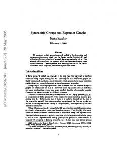
This notation might seem excessive at the moment as the set P κ really only depends on l, and not on κ. However, once we start considering residues of nodes of multipartitions, dependence on κ will become crucial. The Young diagram of the multipartition µ = (µ(1) , . . . , µ(l) ) ∈ P κ is {(a, b, m) ∈ Z>0 × Z>0 × {1, . . . , l} | 1 ≤ b ≤ µa(m) }. The elements of this set are called the nodes of µ. More generally, a node is an element of Z>0 × Z>0 × {1, . . . , l}. Usually, we identify the multipartition µ with its Young diagram and visualize it as a column vector of Young diagrams. For example, ((3, 1), ∅, (4, 2)) is the Young diagram

∅

To each node A = (a, b, m) we associate its residue, which is defined to be the following element of I = Z/eZ: res A := km + (b − a) (mod e). We refer to the nodes of residue i as the i-nodes. Define the residue content of µ to be X cont(µ) := αresA ∈ Q+ . (3.1) A∈µ


17

Denote

(α ∈ Q+ ). Pακ := {µ ∈ P κ | cont(µ) = α} A node A ∈ µ is called removable (for µ) if µ \ {A} has a shape of a multipartition. A node B 6∈ µ is called addable (for µ) if µ ∪ {B} has a shape of a multipartition. We use the notation µB := µ ∪ {B}.

µA := µ \ {A},

For the example above, the removable nodes are (1, 3, 1), (2, 1, 1), (1, 4, 3), (2, 2, 3), and addable nodes are (1, 4, 1), (2, 2, 1), (3, 1, 1), (1, 1, 2), (1, 5, 3), (2, 3, 3), (3, 1, 3), in order from top to bottom in the diagram. Let µ, ν ∈ Pdκ . We say that µ dominates ν, written µ ν, if m−1 X a=1

|µ(a) | +

c X b=1

(m)

µb

≥

m−1 X

|ν (a) | +

a=1

c X

(m)

νb

b=1

for all 1 ≤ m ≤ l and c ≥ 1. In other words, µ is obtained from ν by moving nodes up in the diagram. Let µ) denotes the F -span of the basis elements {CSν′ ,T′ | ν > µ, S′ , T′ ∈ T (ν)}. µ The basis {CS,T | µ ∈ P, S, T ∈ T (µ)} is referred to as a cellular basis and the algebra H with a cell datum is called a cellular algebra.

Given µ ∈ P, define the cell module S(µ) be a free F -module with basis {CT | T ∈ T (µ)} and the H-action X hCT = rh (S, T)CS (h ∈ H, T ∈ T (µ)), S∈T (µ)

where rh (S, T) are the same as in Definition 5.1(iii) (and are easily checked to be uniquely defined). It is an easy consequence of the axioms that the formula above does define an H-module structure on S(µ). For any µ ∈ P, let ϕµ be the F -bilinear form on S(µ) such that µ (S, S) ϕµ (CS , CT ) = rCS,T

(S, T ∈ T (µ)).

Graham and Lehrer [77, Proposition 2.4] prove that the form ϕµ is symmetric and invariant in the following sense: ϕµ (hx, y) = ϕµ (x, h∗ y)

(h ∈ H, x, y ∈ S(µ)).

The invariance of ϕµ implies that its radical R(µ) is an H-submodule of S(µ). Denote D(µ) := S(µ)/R(µ) (µ ∈ P). In practice, it is often not easy to determine when D(µ) is non-zero. However, we have the following fundamental theorem on cellular algebras: Theorem 5.2. [77] Let H be a cellular algebra as above, and put RP := {µ ∈ P | D(µ) 6= 0}. (i) {D(µ) | µ ∈ RP} is a complete and irredundant set of irreducible H-modules up to isomorphism. (ii) The head of S(µ) is isomorphic to D(µ) for any µ ∈ RP. (iii) The multiplicity dµν := [S(µ) : D(ν)] is 0 unless ν ≤ µ; moreover dµµ = 1 for any µ ∈ RP.


23

The numbers dµν appearing in Theorem 5.2(ii) are called the decomposition numbers and the matrix D = (dµν )µ∈P,ν∈RP is called the decomposition matrix (corresponding to the given cellular structure). Theorem 5.2 shows that the decomposition matrix is unitriangular (although not square in general). Hence, knowing decomposition numbers, one can write the class [D(µ)] of an arbitrary irreducible H-module D(µ) in the Grothendieck group of finite dimensional H-modules as a linear combination of the classes of the cell modules [S(ν)] for ν ≤ µ. In particular, one can compute the dimension of D(µ) in terms of the dimensions of cell modules which are given by dim S(µ) = |T (µ)|. 5.2. Cellular structures on cyclotomic Hecke algebras. Following the work of Murphy [157] in level 1, Dipper, James and Mathas [55] have exhibited cellular algebra structures on all cyclotomic Hecke algebras HdΛ . Versions of these cellular structures for degenerate cyclotomic Hecke algebras are explained for example in [12, section 6]. To describe a Dipper-James-Mathas cellular structure on HdΛ , first of all take P to be Pdκ , the set of l-multipartitions of d defined in section 3.1. Next, for any µ ∈ Pdκ , we take T (µ) to be the set of standard µ-tableaux defined in section 3.2. Let ‘∗’ be the anti-automorphism defined in (2.35). To define a cellular basis, fix for the moment µ = (µ(1) , . . . , µ(l) ) ∈ Pdκ with dm := |µ(m) | for m = 1, . . . , l. The standard parabolic subgroup Σµ ≤ Σd is the row stabilizer of the leading tableaux Tµ introduced in section 3.2. Recalling (2.1) and (2.40), set xµ :=

l Y

m=2

d1 +···+dm−1

Y

r=1

X Tw . Xr − ν(kr ) w∈Σµ

Let S, T ∈ T (µ). Recalling 3.4, define µ CS,T := TwS xµ Tw−1 . T

(5.1)

We now have Theorem 5.3. [55] The datum defined above is a cell datum for HdΛ . Two comments on this theorem. First, we point out that the cell datum given in Theorem 5.3 depends on the fixed tuple κ = (k1 , . . . , kl ), and not just the dominant weight Λ = Λ(κ), cf. (2.12), (2.13). Second, the cellular basis appearing in (5.1) is in general not homogeneous with respect to our grading on the cyclotomic Hecke algebra. Very recently, Hu and Mathas [88] constructed homogeneous cellular bases in cyclotomic Hecke algebras, see section 6.5. 5.3. Specht modules and irreducible modules. Theorem 5.3 and the general theory of cellular algebras described in section 5.1 yield the family of cell modules {S(µ) | µ ∈ Pdκ },

24

ALEXANDER KLESHCHEV

for the cyclotomic Hecke algebra HdΛ , which are usually called Specht modules. By definition, each Specht module S(µ) comes with the cellular basis {CT | T ∈ T (µ)}. We note that the definition of the Specht module depends on our fixed tuple κ. We also point out that in level 1 the Specht modules defined here are actually dual to the Specht modules used in the older literature such as [91] and [53]. By Theorem 5.2, in order to classify the irreducible HdΛ -modules, we need to be able to select the multipartitions µ for which D(µ) := S(µ)/R(µ) is non-zero. In level 1 this has been done by James [91] for ξ = 1 and Dipper and James [53] for ξ 6= 1. In higher levels however, this turns out to be an arduous task. At the moment the only approach known to work in full generality relies on Ariki’s Categorification Theorem, and so it is proved rather late in the theory. Having said that, let us state the result here, as it fits naturally into the general theory of cellular algebras. Recall the class RP κ of restricted partitions introduced in section 3.4. Theorem 5.4. Let µ ∈ Pdκ . Then D(µ) 6= 0 if and only if µ ∈ RP κd . In particular, {D(µ) | µ ∈ RP κd } is a complete and irredundant set of irreducible HdΛ -modules up to isomorphism. Theorem 5.4 first appears in [4] (although compare a combinatorial claim made in the proof of [4, Theorem 3.4(2)] with examples in [40, section 3.5]). Another proof is given in [40, Theorems 5.12 and 5.17]. There is a more elementary approach to the classification of irreducible HdΛ modules based on the socle branching rules, see [81] and [125]. In that approach, discussed in detail in section 11.2, one gets hold of irreducible modules over HdΛ inductively using the socles of the restrictions of the irreducible modules to Λ . Unfortunately, it is far from obvious that both approaches lead to the Hd−1 same labeling of irreducible modules, although this is known to be true, see section 11.2 for details. Remark 5.5. Assume that l = 1 and ξ = 1. Then, by Example 3.2(i), the set RP κd consists of the e-restricted partitions of d. Recall that the Specht module S(µ) used here is dual to the Specht module S µ used in James’ book [91]. To see the relation between our D(µ) and the irreducible modules D µ from [91], one uses [91, Theorem 8.15] to deduce Dµ ∼ = D(µt ) ⊗ sgn, where sgn is the sign representation and µt is the partition obtained from µ by transposing with respect to the main diagonal. A similar relation holds in the case where l = 1 and ξ 6= 1, with D µ as in [53]. 5.4. Blocks again. Now that we have explicit constructions of Specht modules and an explicit labeling of irreducible modules we can explain how these modules split into equivalence classes according to the blocks of HdΛ . Recall


25

from section 2.9 that for any α ∈ Q+ of height d we have defined a primitive central idempotent eα , which could be zero, and the corresponding block algebra HαΛ = eα HdΛ . Theorem 5.6. Let µ ∈ Pdκ , ν ∈ RP κd , and α ∈ Q+ be of height d. (i) We have eα 6= 0 if and only if there is λ ∈ Pdκ such that cont(λ) = α. (ii) The Specht module S(µ) belongs to the block HαΛ if and only if cont(µ) = α. (iii) The irreducible module D(ν) belongs to the block HαΛ if and only if cont(ν) = α The proof of this theorem involves identifying the blocks of Specht modules, which is easy to do since their formal characters are known. In fact, it suffices to know that S(µ) is in a fixed block, and then to determine only one weight of S(µ), which can be easily done, see for example [42, Lemma 4.1]. 6. Graded modules over cyclotomic Hecke algebras In this section we begin to systematically take gradings into account. In particular, we explain how to grade irreducible modules and Specht modules in a consistent way. 6.1. Graded irreducible modules. Since HdΛ is a finite dimensional graded algebra, it follows from general principles explained in section 2.2 that the irreducible modules D(µ) are gradable uniquely up to a grading shift. It has been pointed out by Khovanov and Lauda [113, section 3.2] that there is always a preferred choice of the shift which makes the modules self-dual with respect to the graded duality ⊛ defined in section 2.8. To be more precise: Theorem 6.1. [40, Theorem 4.11] For each µ ∈ RP κ , there exists a unique grading on D(µ) which makes it into a graded HdΛ -module such that D(µ)⊛ ∼ = D(µ). Moreover, the modules {D(µ)hmi | µ ∈ RP κ , m ∈ Z} give a complete and irredundant set of irreducible graded HdΛ -modules. Next, we would like to grade Specht modules so that the natural surjection S(µ)։D(µ) is a homogeneous map. This cannot be deduced from general theory, and so Specht modules have to be graded ‘by hand’. 6.2. Homogeneous bases of Specht modules. Let us fix a reduced decomposition for each element w of the symmetric group Σd : w = s r1 . . . s rm , which we refer to as a preferred reduced decomposition of w. We define the elements ψw := ψr1 . . . ψrm ∈ HdΛ (w ∈ Σd ). Since the ‘Coxeter relation’ (2.24) for ψr ’s could have an ‘error term’, in general, ψw depends on the choice of a preferred reduced decomposition of w.

26

ALEXANDER KLESHCHEV

Let µ ∈ Pdκ . We want to define a basis of the Specht module S(µ) which is better adapted to the weight space decomposition and the grading than the cellular basis {CT | T ∈ T (µ)}. Recall the leading tableau Tµ and the elements wT defined in section 3.2. For any µ-tableau T define the vector vT := ψwT CTµ ∈ S(µ).

(6.1)

For example, vTµ = CTµ . Just like the elements ψw , the vectors vT in general depend on the choice of preferred reduced decompositions in Σd . Recall the Bruhat order ≤ on T (µ) defined in section 3.2. The following theorem describes a connection between the vectors vT and the vectors CT , and gives some nice properties of the vectors vT similar to those that CT are known to possess. Theorem 6.2. [42] Let µ ∈ Pdκ . Then (i) For any µ-tableau T we have X aS CS vT =

(aS ∈ F ).

S∈T (µ), S≤T

Moreover, if T is standard, then aT 6= 0. (ii) {vT | T ∈ T (µ)} is a basis of S(µ). Moreover, for any µ-tableau T, we have X vT = bS vS (bS ∈ F ). S∈T (µ), S≤T

The first advantage of the vectors vT over the vectors CT is that they are actually weight vectors: Lemma 6.3. [42] Let µ ∈ Pdκ and T be a µ-tableau. Then vT is an element of the weight space S(µ)iT = e(iT )S(µ). The second advantage of the vectors vT is that they turn out to be homogeneous with respect to a grading of S(µ) as an HdΛ -module. To explain this, recall the notion of the degree deg(T) of a standard tableaux T introduced in section 3.3. Define the degree of vT to be deg(vT ) := deg(T). As {vT | T ∈ T (µ)} is a basis of S(µ), this makes S(µ) into a Z-graded vector space. Since the vectors vT in general depend on the choice of preferred reduced decompositions, our grading on S(µ) might also depend on it. However, the following theorem shows that it does not! Theorem 6.4. [42] Let µ ∈ Pdκ and T ∈ T (µ). If wT = sr1 . . . srm = st1 . . . stm are two reduced decompositions of wT , then ψr1 . . . ψrm CTµ − ψt1 . . . ψtm CTµ =

X

S

aS vS

T

S∈T (µ), S0 ),

(7.21)

(i ∈ I, n ∈ Z>0 ),

(7.22)

and the additive functors (n)

(n)

Ei , Fi

, Ki : Proj(H Λ ) → Proj(H Λ )

7.6. Graded branching rules for irreducible modules. As usual we work with a fixed Λ ∈ P+ of level l. The original branching rules for irreducible modules over symmetric groups in characteristic p were developed in [119]– [124] and [29]. This case corresponds to l = 1 and ξ = 1. In characteristic zero this goes back to a 1908 paper of Schur [178, p. 253]. These branching rules were generalized in various directions, see for example [27, 81, 82, 6, 56, 41, 18, 31, 132, 86, 187, 193, 176, 48, 8, 58]. The graded case is dealt with in [40]. Recall the reduced signatures, good nodes, and other related notions introduced in section 3.4. We point out that all of these combinatorial notions depend on κ. Parts (i),(ii),(iv) of the next theorem go back to [121, 124], and part (iii) to [81]. Theorem 7.4. [40, Theorem 4.12] For any µ ∈ RP κα and i ∈ I, we have:


33

(i) Ei D(µ) is non-zero if and only if εi (µ) 6= 0, in which case Ei D(µ) has irreducible socle isomorphic to D(˜ ei µ)hεi (µ) − 1i and head isomorphic to D(˜ ei µ)h1 − εi (µ)i. (ii) Fi D(µ) is non-zero if and only if ϕi (µ) 6= 0, in which case Fi D(µ) has irreducible socle isomorphic to D(f˜i µ)hϕi (µ) − 1i and head isomorphic to D(f˜i µ)h1 − ϕi (µ)i. (iii) In the Grothendieck group we have that X [Ei D(µ)] = [εi (µ)] · [D(˜ ei µ)] + uν,µ;i (q) · [D(ν)], ν∈RP κ α−αi εi (ν) 1, F (κ) was first studied in [96]. We note that the Fock space F (κ) is simply the tensor product of l level one Fock spaces: F (κ) = F (Λk1 ) ⊗ · · · ⊗ F (Λkl ),

(8.14)

on which the Uq (g)-structure is defined via the comultiplication ∆, so that Mµ is identified with Mµ(1) ⊗ · · · ⊗ Mµ(l) for each µ = (µ(1) , . . . , µ(l) ) ∈ P κ . Theorem 8.1. [40, Theorem 3.26] There is a compatible bar-involution on F (κ) such that Mµ = Mµ + (an A -linear combination of Mν ’s for ν 0. If m < p then the adjustment matrix AΛ α is the identity matrix. The reader is referred to [72, §2] and [61] for further comments and results on James Conjecture. For example Fayers [61] proves that the assumption m < p is essentially the best possible. For a parallel theory for algebraic groups, see [1]. Recalling the notion of defect def(α) from (3.10), it is not hard to observe that in the case Λ = Λ0 , we have m = def(α), cf. [60]. So one could speculate the following generalization beyond level 1: Conjecture 10.8. (Higher Level James Conjecture) Let F be of characteristic p > 0. If def(α) < p, Λ then the adjustment matrix Aα is the identity matrix. A less bold speculation is obtained if we assume def(α) < p/l in the conjecture above. More developments and partial results related to James Conjecture can be found in [61, 62, 72, 73, 74].

50

ALEXANDER KLESHCHEV

11. Some other results In this section we review some other important results which are representative of how representation theory of symmetric groups has been developing in the last fifteen years. 11.1. Blocks of symmetric groups: Brou´ e’s conjecture and ChuangRouquier equivalences. Block theory of finite groups is an extremly vibrant area of research nowadays. General conjectures of Alperin, Broué, Dade and others on the structure of blocks and on relations between arithmetic invariants of blocks provide the main motivation for research, while symmetric groups and their double covers are often the main testing ground for general conjectures. In this section we discuss Broué-type conjectures for symmetric groups, which were recently proved by Chuang and Rouquier in the spectacular paper [48]. The idea is that even though there are very many blocks around, many of them seem to have much in common. So one tries to look for some sort of equivalence between blocks whose invariants coincide. Ideally, these will be Morita equivalences, as in the results of Scopes [179], Kessar [111] and ChuangKessar [47]. However, it is often the case that coarser block invariants (such as Cartan invariants, cf. [33, 84]) coincide, but for example decomposition numbers do not. So one cannot expect a Morita equivalence to hold in general. Instead, Broué and Rickard have suggested weaker versions of equivalence, such as perfect isometry, derived equivalence, stable equivalence, etc., see for example [25, 169, 170]. The famous abelian defect group conjecture of Broué claims that a p-block of a finite group G with abelian defect group D should be derived equivalent to its Brauer correspondent in NG (D) (over a suitable local ring with field of fractions of characteristic 0 and residue field of characteristic p). Thus, in the case of a block B of the symmetric group Sd of p-weight ω < p, there should be a derived equivalence between B and the group algebra of the wreath product (Cp ⋊ Cp−1 ) ≀ Sω . We note that somewhat mysteriously the assumption on p coming from the Broué Conjecture agrees with the assumption on p in the James Conjecture, see section 10.4. In view of the work of Marcus [146] and Chuang-Kessar [47], this conjecture for the case of symmetric groups follows from a conjecture of Rickard (which Rickard himself has proved for p-weights ≤ 5). The following result simply says that Rickard’s Conjecture is true: Theorem 11.1. [48] All blocks of symmetric groups with a fixed p-weight are derived equivalent. Note that this result has a very natural interpretation in terms of the categorification described in section 9.2. Recall that under the categorification the blocks of the symmetric groups correspond to the weight spaces of the module V (Λ0 ). It is easy to see that two blocks have the same p-weight if and only if they belong to the same W -orbit, where W is the Weyl group of g acting naturally on the weights of V (Λ0 ). So the Chuang-Rouquier derived equivalences simply ‘lift’ the action of the Weyl group W from Grothendieck groups to derived categories.


51

Note also that, unlike in Broué’s conjecture, there is no restriction ω < p in Theorem 11.1. We also point out that the work [48] is much more general than Theorem 11.1 might suggest. It develops a general set-up called sl2 -categorification which allows one to deduce results like Theorem 11.1 by checking some rather short and elegant set of axioms. These ideas were developed even further in [174] and [115]. The methods of [48] can be thought of as far-reaching generalizations of the theory developed in [81, 120, 121]. We finish this section by saying that block theory of symmetric groups and related areas have received a lot of attention recently. We refer the interested reader to the following literature for more information: [188, 49, 50, 133, 46, 51, 63, 166, 167, 93, 162, 163, 147, 186, 94, 78, 59, 79, 153, 149, 148, 67, 69, 172]. 11.2. Branching and labeling of irreducible modules. In this section we work in the ungraded setting. A ‘combinatorics-free’ approach to branching rules has been implemented by Grojnowski [81]. This approach ultimately can be used to label irreducible HdΛ -modules. To be more precise, denote by B(Λ) the set of the isomorphism classes of the irreducible HdΛ -modules for all d ≥ 0. Let D be an irreducible HdΛ -module and i ∈ I. Grojnowski and Vazirani [82] give a direct elementary argument to show that either Ei D is zero or it has a simple socle. A similar result holds for the Fi ’s. In level 1, these facts go back to [120, 121]. Set ˜i D := soc (Ei D), F˜i D := soc (Ei D) E (i ∈ I). Thus we get operations ˜i , F˜i : B(Λ) → B(Λ) ⊔ {0}. E For any D ∈ B(Λ) and i ∈ I define εi (D) := max{m | Eim D 6= 0},

ϕi (D) := max{m | Fim D 6= 0}.

Finally, there is a natural weight function wt, defined in terms of central P characters, which associates to any element of B(Λ) a weight of the form Λ− i∈I ci αi , see [81, section 12]. A key result then is as follows Theorem 11.2. [81, Theorem 14.3] The tuple (B(Λ), E˜i , F˜i , εi , ϕi , wt) is the highest weight crystal associated to V (Λ). Now one can bring combinatorics in: Theorem 8.2(ii) gives an explicit combinatorial description of the highest weight crystal associated to V (Λ) in terms of restricted multipartitions. So to every µ ∈ RP κd one can associate an irre˙ ducible module D(µ), and then ˙ {D(µ) | µ ∈ RP κ } d Λ Hd -modules.

is a complete irredundant set of irreducible ˙ ˙ Note that the definition of D(µ) is essentially inductive: we define D(µ) ˙ as the head of Fi D(˜ ei µ) for any i such that e˜i µ 6= 0. This description is very different in nature from the definition of D(µ) as the head of the explicit Specht

52

ALEXANDER KLESHCHEV

module S(µ) over HdΛ , given in Theorem 5.4. This explains why the natural conjecture that ∼ ˙ D(µ) (µ ∈ RP κ ) (11.1) = D(µ) is not easy to prove. This has been first established by Ariki in [6]. Another argument (in the graded setting) is given in [40, Theorems 5.13, 5.18]. Both arguments ultimately depend on the whole power of the theory explained in this exposition. It would be interesting to find a more elementary and direct approach for identifying the two labelings of irreducible modules. 11.3. Extremal sequences. In this section we collect some graded analogues of the results proved in [34], which are quite useful in many situations. For example, Corollary 11.5 has been used in [40] to settle the labeling problem (11.1). See also [142] for another application. For an HdΛ -module M we denote εi (M ) := max{m | Eim M 6= 0}. For example, εi (D(µ)) = εi (µ) by Theorem 7.4(iii). The following result provides an inductive tool for finding certain composition multiplicities. Lemma 11.3. [34, Lemma 2.13] Let M ∈ Rep(HdΛ ), ε = εi (M ), and µ ∈ RP κd−ε . If (ε)

[Ei M : D(µ)] 6= 0 then f˜iε µ 6= 0 and

(ε) [M : D(f˜iε µ)] = [Ei M : D(µ)].

Given i = (i1 , . . . , id ) ∈ I d we can gather consecutive equal terms to write it in the form i = (j1m1 . . . jrmn ) (11.2) 3 2 where js 6= js+1 for all 1 ≤ s < n. For example (2, 2, 2, 1, 1) = (2 1 ). Now, for an HdΛ -module M , the tuple (11.2) is called extremal for M if m

s+1 ms = εjs (Ejs+1 . . . Ejmnn M )

for all s = n, n − 1, . . . , 1. By definition e(i)M 6= 0 if i is extremal for M . The main result about extremal tuples is Theorem 11.4. [34, Theorem 2.16] Let i = (i1 , . . . , id ) = (j1m1 . . . jnmn ) be an extremal tuple for an irreducible HdΛ -module D(µ). Then µ = f˜id . . . f˜i1 ∅, and dim e(i)D(µ) = [m1 ]! . . . [mn ]!. In particular, the tuple i is not extremal for any irreducible D(ν) ∼ 6 D(µ). = This result can be used to compute certain composition multiplicities as follows:


53

Corollary 11.5 ([34, Corollary 2.17]). If i = (i1 , . . . , id ) is an extremal sequence for M ∈ Rep(RdΛ ) of the form (11.2), then µ := f˜id · · · f˜i1 ∅ is a welldefined element of RP κd , and [M : D(µ)]q = (qdim e(i)M )/([m1 ]! . . . [mn ]!). Since the q-characters of Specht modules are known, Corollary 11.5 is especially easy to use to compute some decomposition numbers by induction, see [34] for details. 11.4. More on branching for symmetric groups. We draw the reader’s attention to the fact that in level one, the original modular branching rules of [119]–[124] and their generalizations [27, 29], give much more information than just a description of the socles of the restrictions of irreducible modules. It would be interesting to have similar more general results in higher levels. Here we state the results for the symmetric groups only, and in the ungraded setting. Assume that the characteristic of the ground field F is p > 0, Λ = Λ0 and ξ = 1. Then and e = p. We know from Theorem 5.4 and Example 3.2(i) that the irreducible F Σd -modules D(µ) are labeled by the p-restricted partitions µ of d. We now slightly generalize the combinatorics of section 3.4 in this particular case. Let i ∈ I = Z/pZ, and σ be the reduced i-signature of µ. Recall that the i-node corresponding to leftmost − in σ is called the good i-node of µ, while the addable i-node corresponding to rightmost + in σ is called the cogood i-node for µ. Moreover, the removable i-nodes corresponding to the −’s in σ are called the normal i-nodes of µ, while the addable i-nodes corresponding to the +’s in σ are called the conormal i-nodes for µ. Thus the good i-node is the top normal i-node, while the cogood i-node is the bottom conormal i-node. Also, εi (µ) is the number of the normal i-nodes of µ, while ϕi (µ) is the number of the conormal i-nodes for µ. The additional branching results not covered by Theorem 7.4, are now as follows. Theorem 11.6. [120, 123] Let µ be a p-restricted partition of d, and ν be a p-restricted partition of d − 1. (i) HomΣd−1 (S(ν), Ei D(µ)) 6= 0 if and only if ν = µA for some normal i-node A of µ. (ii) Suppose ν = µA for some removable i-node A of µ. Then the multiplicity [Ei D(µ) : D(ν)] 6= 0 if and only if A is normal for µ, in which case [Ei D(µ) : D(ν)] is the number of normal i-nodes weakly below A (counting A itself ). Theorem 11.7. [29] Let µ be a p-restricted partition of d, and ν be a prestricted partition of d + 1. (i) HomΣd+1 (S(ν), Fi D(µ)) 6= 0 if and only if ν = µB for some conormal i-node B for µ. (ii) Suppose ν = µB for some addable i-node B for µ. Then the multiplicity [Fi D(µ) : D(ν)] 6= 0 if and only if B is conormal for µ, in which case [Fi D(µ) : D(ν)] is the number of conormal i-nodes weakly above B (counting B itself ).

54

ALEXANDER KLESHCHEV

The additional branching information provided by Theorems 11.6, 11.7 turns out very useful in applications, see for example [15, 14, 30, 57, 131, 94, 177, 66, 196, 95, 134]. 11.5. Mullineux Involution. The algebra Hd has an automotphism σ : Hd → Hd , Tr 7→ −Tr + ξ − 1

(1 ≤ r < d).

Twisting an irreducible Hd -module D(µ) yields an irreducible module D(µ)σ . For the symmetric groups we simply have D(µ)σ ∼ = D(µ) ⊗ sgn, where sgn is the one-dimensional sign representation of Σd . The involution σ arises in many natural situations. For example, one needs to deal with it when studying representation theory of alternating groups. Another illustration comes from Remark 5.5. The next result provides an explicit combinatorial algorithm for computing the involution σ in terms of the combinatorics of good nodes. Theorem 11.8. [121] Let µ be an e-restricted partition of d. Write µ = f˜i f˜i . . . f˜i ∅ 1

for some i1 , i2 , . . . , id ∈ I. Then

2

d

∼ = D(ν), where f˜−i . . . f˜−i ∅.

(11.3)

D(µ)σ

ν = f˜−i1

2

d

(11.4)

It is implicit in the theorem above that there always exists a presentation of µ in the form (11.3) starting with the empty partition ∅ and that the formula (11.4) determines a well-defined e-restricted partition. Indeed, to find a presentation of µ in the form (11.3) one should consecutively remove good nodes from µ and record their residues in order of removal: i1 , i2 , . . . , id . Then one should build ν by consecutively adding good nodes of residues −id , . . . , −i2 , −i1 . Originally, Mullineux [154] conjectured a different description of the involution D(µ) 7→ D(µ)σ . It has been shown in [68] that that description is equivalent to the one given in Theorem 11.8. Questions related to the Mullineux involution received quite a lot of attention. We refer the reader to [27, 17, 197, 43, 139, 64, 87, 163, 19, 16, 90, 65, 183] as well as [40, Remarks 3.17, 3.18] and [39, section 3.7] for further information. 11.6. Higher level Schur-Weyl duality, W -algebras, and category O. Throughout this section we assume that ξ = 1 and F = C. In this case, there is quite a different approach to representation theory of HdΛ based on a generalization of Schur-Weyl duality. This duality connects representation theory of the cyclotomic Hecke algebra HdΛ with that of a finite W -algebra and ultimately with a parabolic category O. We review the main features of that theory here referring the reader to [37, 39] for details. Using shifts of the elements Xr ∈ HdΛ by the same scalar k1 , we may assume without loss of generality that in (2.12) we have 0 = k1 ≥ k2 ≥ · · · ≥ kl . Let n ≥ −kl , and define qm := n + km

(1 ≤ m ≤ l).


55

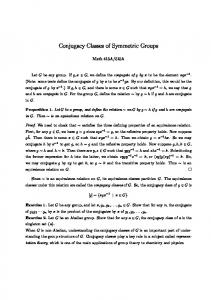
Then (q1 , . . . , ql ) is a partition. Let q1 +· · ·+ql = N , and let λ = (p1 ≤ · · · ≤ pn ) be a partition of N transposed to (q1 , . . . , ql ). Unlike in the main body of the paper, it is convenient to identify λ with its Young diagram in an unusual way, numbering rows by 1, 2, . . . , n from top to bottom and columns by 1, 2, . . . , l from left to right, so that there are pi boxes in the ith row and qj boxes in the jth column. For example, for Λ = 2Λ0 + Λ−1 + Λ−2 and n = 3, we have λ = (p1 , p2 , p3 ) = (2, 3, 4), (q1 , q2 , q3 , q4 ) = (3, 3, 2, 1), N = 9. The Young diagram is 1 4 2 5 7 3 6 8 9 . We always number the boxes of the diagram 1, 2, . . . , N down columns starting from the first column, and write row(i) and col(i) for the row and column numbers of the ith box. This identifies the boxes with the standard basis v1 , . . . , vN of the natural glN (C)-module V . Define e ∈ glN (C) to be the nilpotent matrix of Jordan type λ which maps the basis vector corresponding the ith box to the one immediately to its left, or to zero if there is no such box; in our example, e = e1,4 + e2,5 + e5,7 + e3,6 + e6,8 + e8,9 . Finally, define a Z-grading M glN (C) = glN (C)r r∈Z

on glN (C) by declaring that ei,j is of degree col(j) − col(i) for each i, j = 1, . . . , N , and set M M p= glN (C)r , h = glN (C)0 , m = glN (C)r . r